The Concrete Effective Width of a Composite I Girder with Numerous Contact Points as Shear Connectors


1
Faculty of Civil Engineering, Damascus University, Damascus P.O. Box 30621, Syria
2
L2MGC—Civil Engineering Mechanics and Materials Laboratory, CY Cergy-Paris University, 95031 Neuville-sur-Oise, France
*
Author to whom correspondence should be addressed.
Appl. Mech. 2024, 5(1), 163-179; https://doi.org/10.3390/applmech5010011
Submission received: 14 December 2023
/
Revised: 15 February 2024
/
Accepted: 27 February 2024
/
Published: 7 March 2024
(This article belongs to the Special Issue Feature Papers in Applied Mechanics (2nd Volume))
Abstract
:Due to the shear strain in the plane of the slab, the parts of the slab remote from the steel beam lag behind the part of the slab located in its proximity. This shear lag effect causes a non-uniform stress distribution across the width of the slab. As a result, several standards have introduced the concept of an effective flange width to simplify the analysis of stress distribution across the width of composite beams. Both the computed ultimate moment and serviceability limit states are directly impacted by the effective width. The effect of using a large number of contact points as shear connectors on the effective width of a steel beam flange has not been investigated. A three-dimensional finite element analysis is carried out in this paper. The ABAQUS software (version 6.14) is used for this purpose, where several variables are considered, including the surface area connecting the steel beam and concrete slab, the transverse space, and the number of shear connectors. It was discovered that the number of shear connectors on the steel beam flange has a major impact on the effective width. The many connectors work together to provide a shear surface that improves the effective width by lowering the value of the shear lag.
1. Introduction
An effective flange width is a concept that simplifies the calculation of flange bending stresses required to determine the ultimate moment capacity of composite beams [1,2,3,4]. An effective slab width, rather than the actual width or steel beam spacing, is the theoretical basis for design calculations. The parts of the slab furthest from the steel beam will lag behind those closer due to shear strain in the plane of the slab, resulting in an uneven stress distribution across the width. The transfer of shear from the studs (welded to the top flange of the steel beam) to the concrete slab becomes less effective as the beam spacing increases [5]. Many researchers are still investigating the accuracy of effective flange width calculation despite the number of prediction models proposed by design standards. The computation of the shear, moment, torque, composite beam properties, and the necessary shear connectors are all directly impacted by the estimation of this width [6,7].
The impact of connector numbers and positions on the effective width of a composite beam flange has not yet been fully explored [8,9,10]. The effective width of a flange is the width of a hypothetical flange that compresses uniformly across its width, similar to the loaded edge of a real flange under the same edge shear forces. This can be viewed as the theoretical flange carrying a compression force with uniform stress equal to the peak stress at the prototype wide flange edge (Figure 1) [11]. The simple bending theory will provide the correct value of the maximum stress (at point C) if the true flange width is replaced by an effective width, provided the area ABCDE equals the area FHCIG.
Additionally, depending on which design parameter is considered more significant, the effective width can be defined in a variety of ways. It is generally obtained by integrating the strictly calculated longitudinal stress in the slab at the top or mid-surface and then dividing it by the peak stress value. In composite systems, the horizontal shear transmitted at the interface is regarded as more significant than the flexing of the slab. Therefore, it is calculated here by considering the top surface stress, and the width is given by [11,12]
is the one-side effective slab width.
σx represents the normal stress in the longitudinal direction.
(σx)max is the maximum normal stress of 0 ≤ y ≤ b
The variation in compressive strains and stresses over the slab thickness, as shown by Aref et al. [13,14], was a drawback of using Equation (1) to derive the effective flange width. As a result, depending on where strain/stress distributions are measured, different values of the effective flange width will be produced. The authors described a new effective width flange beam using the following expression, which is particularly simple for analyzing structures like thin plates and shells [13].
where beff = the total effective slab width for one girder, Cslab = the total compressive force in the slab, F = the force per unit width of the slab, tslab = the total slab thickness subjected to compression, σmax = the maximum slab compressive stress, and σmin = the minimum slab compressive stress.
A nonlinear finite element analysis has been conducted in the investigation and development of a more versatile and effective flange width definition for single-span bridges.
Nassif et al. [15] carried out an experimental and analytical work program, which consisted of the casting and testing of eight composite steel beam specimens. Three parameters were considered: (1) the concrete slab width, (2) the percentage of shear connectors, and (3) the steel beam section. All of the beams under the test had the same span, and powerful simple equations were the result of the experimental and analytical work in this study. In addition, they concluded that the number of shear connectors has a significant effect on the effective width of the flange. A reduction in the number of shear connectors in comparison to the full shear interaction required by the design standard resulted in a reduction in the effective width of the flange. Furthermore, the important role of the degree of shear interaction in composite beams had been long qualified by Gjelsvik [16] and U. Girhammar et al. [17,18,19], but they did not mention the effective width.
Yang et al. [2] focused on the effective width to calculate the deflection of composite beams. Theoretical models were first developed, and the interface slip and shear lag effect were considered. The comparison of the predictions of the theoretical model with those of the finite element model indicates that the theoretical model can accurately predict the behavior of the composite beam. Finally, they proposed a simplified set of design formulas to calculate the effective width of a steel–concrete composite T-beam.
x1 reflects the influence of the beam span.
x2 accounts for the effects of the slab thickness.
b represents the width of the concrete slab, L is the span of the beam, and hc is the thickness of the floor slab.
is the coefficient of the effective width.
be′ is the effective width.
The shear lag phenomenon in steel–concrete composite beams was studied by Al-Sherrawi and Mohammed [11]. Parametric studies have been carried out to investigate the effect of some important parameters in a composite beam under a concentrated load; these parameters included the degree of interaction, concrete compressive strength, and longitudinal reinforcement of the slab. The variation in these parameters has effects on the shear lag and the effective slab width. In the study by Lasheen et al. [3], different parameters related to beam geometry and concrete slab material were considered for the evaluation of effective slab widths at service and ultimate loads. The results of this study showed that the effective width depended on the slenderness ratio (L/rs) of the steel beam and the slab width-to-span ratio (Bs/L). In addition, it was found that the effective width at the ultimate load was wider than that at the service load.
The effects of the ratio of beam spacing to span size and the type of loading on the effective flange widths of composite beams were investigated by Yam and Chapman [20]. The research based on elastic theory has shown that the beff/bs ratio depends on the bs/L ratio and the boundary conditions at the supports, where bs is the slab width and L is the beam span. In addition, Fahmy and Robinson [21] found that the effective flange width increased with the increasing number of flexible shear connectors using a combination of finite difference and layered finite element methods to analyze composite beams. The effective flange width of a composite beam was also affected by the loading pattern.
Previous research studies show that the effective width is a problematic issue that researchers focus on [8]. Several equations are proposed, but none of the studies investigated the effect of using multiple connectors on the effective width of the steel beam flange, the transverse spacing, the location of the shear connectors, and the surfaces that connect the steel beam to the concrete slab. The main objective of this paper is to evaluate the effect of using several points as shear connectors on the effective flange width of composite beams at the limit states.
2. Materials and Methods
2.1. Finite Element Model
ABAQUS software version 6.14 [22] was used to evaluate the distribution of stresses in the concrete slab for simply supported composite beams. In the present study, the selected beam was referred to as the beam (E11) from the series tested by Yam and Chapman [20]. The beam had a span of 5486 mm and was subjected to a concentrated load at the midspan. The composite beam E11 has 100 studs, 2 in each section, with a longitudinal spacing of 100 mm. The total length of the studs is 50 mm, and their diameter is 12 mm. The dimensions and reinforcement details of this beam are shown in Figure 2.
The material properties of the Yam and Chapman composite beam are summarized in Table 1. Initially, two FE models were proposed and analyzed. The first model has four components: a steel beam, a concrete slab, and studs and reinforcing bars (Figure 3). The second model consists of three components: reinforcing bars, a steel beam, and a concrete slab. In the second approach, the connectors are represented as element connectors (Figure 4). The connector section is an MPC (multi-point constraints)-type beam. A connector was created between two corresponding points. The multi-point constraint (MPC) is the option used to impose constraints between different degrees of freedom of the model. The MPC-type beam provides a rigid beam between two nodes to constrain the displacement and rotation at the first node to the displacement and rotation at the second node, corresponding to the presence of a rigid beam between the two nodes. More details can be found in the ABAQUS Analysis User’s Manual 28.2.2 General regarding multi-point constraints [22]. Figure 5 illustrates the MPC connectors. The three-dimensional eight-node solid element C3D8R [23,24,25,26] is used to model the steel beam, the concrete, and the studs, whereas the truss element T3D2 is used to simulate the steel rebar. The lines in Figure 4 are not mesh lines, but partition lines. Part partition was used to mesh the model easily because the model contains circular surfaces. The meshing of finite elements was performed by refining the finite elements and iterating the solution until a stable and accurate result was obtained.
The geometric and material nonlinear analysis was performed in a quasi-static manner using the dynamic explicit solver, as it does not have the usual convergence problems of an implicit static solver. The explicit dynamics procedure was originally developed to model high-speed impact events. Explicit dynamics solve for the state of dynamic equilibrium where inertia plays a dominant role in the solution. The application of explicit dynamics to model quasi-static events requires the following special considerations:
- It is computationally impractical to model the process in its natural time.
- Artificially increasing the speed of the process in the simulation is necessary to obtain an economical solution.
- An examination of the energy content provides a measure to evaluate whether the results from an ABAQUS/Explicit simulation reflect a quasi-static solution. The kinetic energy of the deforming material should not exceed a small fraction of its internal energy throughout the majority of a quasi-static analysis (typically 1–5%).
- Smooth step amplitude curves should be used to improve the early response. The computation time of a real-time quasi-static analysis can be prohibitively long, so the computation speed can be increased by either time scaling or mass scaling. These techniques tend to increase the forces of inertia in a model; however, in these analyses, mass scaling was employed with a smooth step at a desired time increment of 0.001 s to minimize inertia. The beam’s symmetry has been considered in modeling only its half. As seen in Figure 6, the center of the beam was subjected to symmetric boundary constraints via limited displacement in the z-axis for every node and rotation in the x-axis slab elements. The beam’s extremity’s bottom steel flange was utilized to simulate roller support through constrained displacement on the y-axis.
A general contact interaction procedure was successfully used by many researchers to model the contact between the concrete and the steel beam, such as M.S. Pavlović [25] and M. Paknahad et al. [27]. A hard contact was used in the normal direction, and a penalty was used with a friction coefficient of 0.45 in the tangential direction [28]. In the present study, the embedded constraint was used to model the contact between the concrete and the reinforcing rebars inside the slab [23,24,26]. Moreover, the studs were tied to the steel flange by using tied constraints in the first model.
The steel section, the reinforcing bars, and the studs were designed using the perfect elastoplastic stress–strain law [27]. The elastic modulus was equal to 205 GPa, the density was γ = 7850 kg/m3, Poisson’s ratio was ν = 0.3, and the yield stress was fy = 265 MPa.
Researchers have proposed many innovative models for concrete, such as Cervenka et al. [29], who used the concrete model based on fracture mechanics for tensile failure and plasticity for compressive failure. In addition, De Maio et al. [30] presented an improved numerical model based on the cohesive fracture approach and the embedded truss model to simulate the nonlinear crack processes and mechanical behavior of rebars. De Maio et al. [31] also suggested an integrated model based on a cohesive crack approach that is employed in combination with a bond–slip model to perform a failure analysis of strengthened structures. In this study, the Concrete Damaged Plasticity (CDP) was the constitutive model used to represent the mechanical behavior of concrete. The failure surface in the deviatoric plane of the CDP model, which is a modification of the Drucker-Prager model, is not a circle and is controlled by a parameter called kc, which is typically equal to 2/3. Four additional parameters are needed for the CDP model: the dilation angleψ; the flow potential eccentricity (ε), which is a small positive number that defines the rate at which the hyperbolic flow potential approaches its asymptote; the ratio of initial biaxial compressive yield stress to initial uniaxial compressive yield stress (fb0/fc0); and the viscosity (referred to as µ). These parameters are shown in Table 2.
According to the model, damaged plasticity describes the two primary failure mechanisms in concrete, namely compressive crushing and tensile cracking. When the elastic stage is reached, the elastic modulus can be expressed as , where d is the plastic damage factor and Ec0 is the initial elastic modulus. The parameter d, also known as dc in compression and dt in tension, has a range of 0 to 1, where 0 denotes no damage to the material and 1 denotes the total loss of strength.
It is necessary to define the compressive stress–strain curve in the form with as the compressive strength and as the inelastic strain, which can be defined as (Figure 7a). ABAQUS automatically converts the crushing strain into a plastic strain based on Equation 4 once the compressive damage data are entered into ABAQUS in the form . A complete description of the compression damage parameter was recently given by Bello et al. [32].
The tensile stress–strain curve is assumed to be linear and described by Hooke’s law until tensile strength is reached. In the post-cracking phase, the difference between the total strain and the elastic strain for the undamaged material is the cracking strain and can be given as (Figure 7b). After defining the tension damage parameter, or dt, the plastic strain is calculated like compression (Equation (5)):
with .
In this study, the relative stress–strain curve of the concrete proposed by Pavlović [25] was adopted, where the envelope was calculated using the analytical model of Eurocode 2 (EC2) up to the ultimate strain εcu1, which was equal to 0.0035 [33]. Additionally, due to the restrained expansion of concrete in front of a shear connector, high compressive stresses are produced in all three orthogonal directions, leading to the confined condition of the concrete. Concrete compression behavior only up to strain ɛcu1 would lead to an unreal overestimation of concrete crushing. For this reason, the EC2 stress–strain curve was extended beyond the nominal ultimate strain. The extension was made as defined by Equation (6) with a sinusoidal part between points D–E and a linear part between points E–F, where F is related to a strain of 10% and a stress of 0.4 MPa [21,30].
In Equation (6), is a relative coordinate between points D–E and . Point D is defined as and .
Point E is the end of the sinusoidal descending part at strain with the concrete strength reduced to by factor /. The linear descending part (residual branch) ends in point F at the strain with the final residual strength of concrete, . Strain was chosen to be large enough so as not to be achieved in the analyses. The final residual strength of concrete, = 0.4 MPa, a reduction factor of , and a strain of = 0.03 were calibrated by Pavlović [25]. Factors and 0.9, governing the tangent angles of the sinusoidal part at points D and E, were chosen to smoothen the overall shape of the concrete’s stress–strain curve. The behavior of the used material is shown in Figure 8a in terms of uniaxial compression stress–uniaxial compression strain. The tensile stress–strain curve was also adopted from Pavlović [25]. The axial tensile strength of concrete, fctm = 4 MPa, was taken from Table 1. After this point, tension softening appeared, induced by the crack opening. Tension stress is degraded in a sinusoidal manner between points B and C until a stress of fctm/20 is achieved at the cracking strain of Ɛtu = 0.001. Such a small value of tensile stress at the end of tension softening (point C), instead of a value of zero, was defined for numerical stability reasons. The tension plasticity curve for input in ABAQUS was defined depending on the cracking strain from point B to C. The strain softening curve is represented in Figure 8b. A detailed description of the concrete behavior can be found in the study by Pavlović [25].
By comparing the results obtained from the finite element analysis program (ABAQUS) with those obtained from the experimental test, the above finite element modeling can be verified. Compared to the reference experiment, the results show a good estimation of the behavior of the implemented finite element models. The difference in mid-span deflection is around 4.5% for the first model and 3.4% for the second, while the difference in the ultimate load is about 0.98% for the first model and 0.5% for the second, as shown in Table 3. These results show the accuracy and efficiency of the selected elements in the ABAQUS software (version 6.14) in predicting the behavior and ultimate load of composite steel–concrete beams. The results of the two models were close. In addition, the modeling of the connectors as MPC elements is more efficient in terms of the computation time. Therefore, the choice of the MPC model for the connectors is justified. The curves are shown in Figure 9.
2.2. Parametric Study
After the finite element model was validated, a parametric study was conducted. The number of shear connectors on the transverse flange steel section, the transverse spacing, the locations of the shear connectors, and the surfaces connecting the concrete slab and steel beam were the study parameters.
First, two MPC-type circular connectors with a diameter of 8 mm instead of 12 mm were selected, as seen in Figure 10, to show the effect of the connected surface in MPC definition. Following that, the two connector MPC-type beams were replaced with four and then seven MPC connectors with the same location and the same surface in the MPC definition, which is circular (diameter = 8 mm), to show the effect of the number of shear connectors on the width of the steel beam flange. The three models are shown in Figure 11. To study the effect of the transverse spacing, Figure 12 and Figure 13 show the locations of shear connectors with two MPCs and four MPCs with different space ratios. The flange width of the steel section is denoted by (bs) in these figures, while (a) stands for the distance between the opposing outside connectors. Two different values were taken for a, 38 mm and 114 mm, respectively, while the flange width was fixed at bs = 152 mm. Hence, two a/bs ratios are obtained, namely 0.25 and 0.75.
3. Results and Discussion
Table 4 summarizes six models that focused on the diameter, the a/bs ratio, and the number of connectors.
The stresses at the top of the slab are depicted in Figure 14, where it is clear that the stresses increase as the diameter of the connector increases from 8 to 12 mm. Furthermore, there are raises when four MPC connectors are used rather than two. The a/bs ratio appears to have a minimal effect on the stress distribution.
Figure 15 illustrates the effect of incorporating more shear connectors on the width of the steel flange beam. It is possible to observe that as the number of shear connectors increases from four to seven, the stresses increase throughout the width of the slab, and the distribution of those stresses becomes more homogeneous.
The effective width was calculated using Equation (1), where the integral was calculated numerically using the trapezoidal method and then the sum was divided by the maximum stress. The effective width for model 6 is 745 mm, whereas for model 5, it is 458 mm according to the computation procedure. Then, this procedure was carried out every 20 cm along the half-span of the beam.
The effective width evolution for two connectors with an a/bs ratio of 0.25 and a diameter variation from 8 mm to 12 mm is shown in Figure 16. The inefficiency of clamping two small diameter connectors is evident from these results. Using a 12 mm diameter, the effective width remains nearly constant throughout a length that accounts for 36% of the half span.
The impact of the number of connectors on the effective width is shown in Figure 17 with an a/bs ratio of 0.75. It can be observed that, as this number increases, the effective width in the mid-span also increases. Moreover, the computed values are not significantly impacted by the change in the a/bs ratio (Figure 18).
The number of shear connectors is the most significant parameter in terms of the effect on the effective width. This is because a semi-surface shear connector is created when a large number of connectors are used across the width of the steel beam flange, which, in turn, increases stresses and the effective width. In addition, increasing the space ratio between the opposite outside connectors and the steel beam flange increases the effective width.
4. Conclusions
To calculate the effective width of a composite beam with several contact points acting as shear connectors, a three-dimensional finite element analysis was carried out in this work using the ABAQUS software. Several variables were considered, including the surface area connecting the steel beam and concrete slab, the transverse spacing, and the number of shear connectors. The results indicate that the test chosen from the bibliography and the numerical analysis accord quite well. While the difference ratio in central deflection is around 3.4%, the difference ratio in the ultimate load is approximately 0.5%.
Following model validation, a parametric analysis was carried out, and the following conclusions can be made in light of the results:
- The number of shear connectors has a significant effect on the effective width; the numerous connectors work together to create a semi-surface shear connector, which increases the effective width by reducing the amount of shear lag. Increasing the number of connectors from four to seven increases the effective width at the mid-span by 62%.
- Expanding the surface area used in the definition of the MPC connector has a significant effect; when the diameter of the circle is raised from 8 mm to 12 mm, the effective width at the mid-span increases.
- For the same number of shear connectors, increasing the space ratio between opposite outer connectors and the steel beam flange has no significant effect.
Author Contributions
A.H., M.S. and G.W. designed the study, wrote the manuscript, and revised the manuscript. Conceptualization, A.H. and G.W.; methodology, A.H. and M.S.; modeling, A.H.; validation, G.W. and M.S.; formal analysis, M.S.; investigation and writing—original draft preparation, A.H.; writing—review and editing, G.W. and M.S.; visualization, A.H. and G.W.; supervision, M.S. All authors have read and agreed to the published version of the manuscript.
Funding
This research received no external funding.
Institutional Review Board Statement
Not applicable.
Informed Consent Statement
Not applicable.
Data Availability Statement
The data that support the findings of this study are available from the first author Alaa HASAN upon reasonable request.
Conflicts of Interest
The authors declare no conflicts of interest.
References
- Amadio, C.; Fragiacomo, M. Effective width evaluation for steel–concrete composite beams. J. Constr. Steel Res. 2002, 58, 373–388. [Google Scholar] [CrossRef]
- Yuan, H.; Deng, H.; Yang, Y.; Weijian, Y.; Zhenggeng, Z. Element-based effective width for deflection calculation of steel-concrete composite beams. J. Constr. Steel Res. 2016, 121, 163–172. [Google Scholar] [CrossRef]
- Lasheen, M.; Shaat, A.; Khalil, A. Numerical evaluation for the effective slab width of steel-concrete composite beams. J. Constr. Steel Res. 2018, 148, 124–137. [Google Scholar] [CrossRef]
- Nie, J.-G.; Tian, C.-Y.; Cai, C. Effective width of steel–concrete composite beam at ultimate strength state. Eng. Struct. 2008, 30, 1396–1407. [Google Scholar] [CrossRef]
- Masoudnia, R. State of the art of the effective flange width for composite T-beams. Constr. Build. Mater. 2020, 244, 118303. [Google Scholar] [CrossRef]
- Men, P.; Liang, B.; He, W.; Di, J.; Qin, F.; Zhang, Z. Vertical shear resistance of noncompact steel–concrete composite girders under combined positive moment and shear. Case Stud. Constr. Mater. 2023, 18, e01835. [Google Scholar] [CrossRef]
- Fang, Z.; Hu, L.; Jiang, H.; Fang, S.; Zhao, G.; Ma, Y. Shear performance of high-strength friction-grip bolted shear connector in prefabricated steel–UHPC composite beams: Finite element modelling and parametric study. Case Stud. Constr. Mater. 2023, 18, e01860. [Google Scholar] [CrossRef]
- He, S.; Yang, G.; Jiang, Z.; Wang, Q.; Dong, Y. Effective width evaluation for HSS-UHPC composite beams with perfobond strip connectors. Eng. Struct. 2023, 295, 116828. [Google Scholar] [CrossRef]
- He, S.; Xu, Y.; Zhong, H.; Mosallam, A.S.; Chen, Z. Investigation on interfacial anti-sliding behavior of high strength steel-UHPC composite beams. Compos. Struct. 2023, 316, 117036. [Google Scholar] [CrossRef]
- Lu, L.; Wang, D.; Ding, K.; Yan, H.; Hao, H. A Proposal for a Simple Method for Determining the Concrete Slab Width of Composite Beam-to-Column Joints. Appl. Sci. 2021, 11, 9613. [Google Scholar] [CrossRef]
- Dawood, A.R.; Al-Sherrawi, M.H. The Effective Width of a Partially Composite Steel-Concrete Beam. Int. J. Adv. Eng. Res. Dev. 2018, 5, 24–31. [Google Scholar]
- Al-Sherrawi, M.H.; Mohammed, S.N. Shear Lag in Composite Steel Concrete Beams. In Proceedings of the 2018 1st International Scientific Conference of Engineering Sciences—3rd Scientific Conference of Engineering Science (ISCES), Diyala, Iraq, 10–11 January 2018; pp. 169–174. [Google Scholar]
- Aref, A.J.; Chiewanichakorn, M.; Chen, S.S.; Ahn, I.-S. Effective Slab Width Definition for Negative Moment Regions of Composite Bridges. J. Bridg. Eng. 2007, 12, 339–349. [Google Scholar] [CrossRef]
- Chen, S.S.; Aref, A.J.; Chiewanichakorn, M.; Ahn, I.-S. Proposed Effective Width Criteria for Composite Bridge Girders. J. Bridg. Eng. 2007, 12, 325–338. [Google Scholar] [CrossRef]
- Thaickavil, N.N.; Thomas, J. Behaviour and strength assessment of masonry prisms. Case Stud. Constr. Mater. 2018, 8, 23–38. [Google Scholar] [CrossRef]
- Betti, R.; Gjelsvik, A. Elastic composite beams. Comput. Struct. 1996, 59, 437–451. [Google Scholar] [CrossRef]
- Girhammar, U.A.; Pan, D.H. Exact static analysis of partially composite beams and beam-columns. Int. J. Mech. Sci. 2007, 49, 239–255. [Google Scholar] [CrossRef]
- Girhammar, U.A.; Pan, D.H.; Gustafsson, A. Exact dynamic analysis of composite beams with partial interaction. Int. J. Mech. Sci. 2009, 51, 565–582. [Google Scholar] [CrossRef]
- Girhammar, U.A.; Pan, D. Dynamic analysis of composite members with interlayer slip. Int. J. Solids Struct. 1993, 30, 797–823. [Google Scholar] [CrossRef]
- Yam, L.P.C.; Chapman, J.C. The inelastic behavior of simply supported composite beams of steel and concrete. Proc. Inst. Civ. Eng. 1968, 45, 651–683. [Google Scholar]
- Fahmy, E.H.; Robinson, H. Effective slab widths for simple composite beams with ribbed metal deck. Model. Simul. Control B 1985, 3, 19–36. [Google Scholar]
- Abaqus Unified FEA, ABAQUS 6.14. Available online: https://www.3ds.com/fr/produits-et-services/simulia/produits/abaqus/ (accessed on 1 December 2023).
- Qin, F.; Huang, Z.; Zheng, Z.; Chou, Y.; Zou, Y.; Di, J. Analytical model for the load-slip relationship of bearing-shear connectors. Front. Mater. 2023, 10, 1110232. [Google Scholar] [CrossRef]
- Ali, Y.A.; Falah, M.W.; Ali, A.H.; Al-Mulali, M.Z.; AL-Khafaji, Z.S.; Hashim, T.M.; AL Sa’adi, A.H.M.; Al-Hashimi, O. Studying the effect of shear stud distribution on the behavior of steel–reactive powder concrete composite beams using ABAQUS software. J. Mech. Behav. Mater. 2022, 31, 416–425. [Google Scholar] [CrossRef]
- Pavlović, M.S. Resistance of Bolted Shear Connectors in Prefabricated Steel-Concrete Composite Decks; University of Belgrade: Belgrade, Serbia, 2013. [Google Scholar]
- Zhu, Z.-H.; Zhang, L.; Bai, Y.; Ding, F.-X.; Liu, J.; Zhou, Z. Mechanical performance of shear studs and application in steel-concrete composite beams. J. Cent. South Univ. 2016, 23, 2676–2687. [Google Scholar] [CrossRef]
- Paknahad, M.; Shariati, M.; Sedghi, Y.; Bazzaz, M.; Khorami, M. Shear capacity equation for channel shear connectors in steel-concrete composite beams. Steel Compos. Struct. 2018, 28, 483–494. [Google Scholar]
- Tahmasbi, F.; Maleki, S.; Shariati, M.; Sulong, N.H.R.; Tahir, M.M. Shear capacity of C-shaped and L-shaped angle shear connectors. PLoS ONE 2016, 11, e0156989. [Google Scholar] [CrossRef]
- Rimkus, A.; Cervenka, V.; Gribniak, V.; Cervenka, J. Uncertainty of the smeared crack model applied to RC beams. Eng. Fract. Mech. 2020, 233, 107088. [Google Scholar] [CrossRef]
- De Maio, U.; Gaetano, D.; Greco, F.; Lonetti, P.; Blasi, P.N.; Pranno, A. The Reinforcing Effect of Nano-Modified Epoxy Resin on the Failure Behavior of FRP-Plated RC Structures. Buildings 2023, 13, 1139. [Google Scholar] [CrossRef]
- De Maio, U.; Gaetano, D.; Greco, F.; Lonetti, P.; Pranno, A. The damage effect on the dynamic characteristics of FRP-strengthened reinforced concrete structures. Compos. Struct. 2023, 309, 116731. [Google Scholar] [CrossRef]
- Bello, I.; González-Fonteboa, B.; Wardeh, G.; Martínez-Abella, F. Characterization of concrete behavior under cyclic loading using 2D digital image correlation. J. Build. Eng. 2023, 78, 107709. [Google Scholar] [CrossRef]
- Européen, C. Eurocode 2: Design of Concrete Structures—Part 1-1: General Rules and Rules for Buildings; British Standard Institution: London, UK, 2004. [Google Scholar]
Figure 1.
Effective flange width definition for positive moment section.
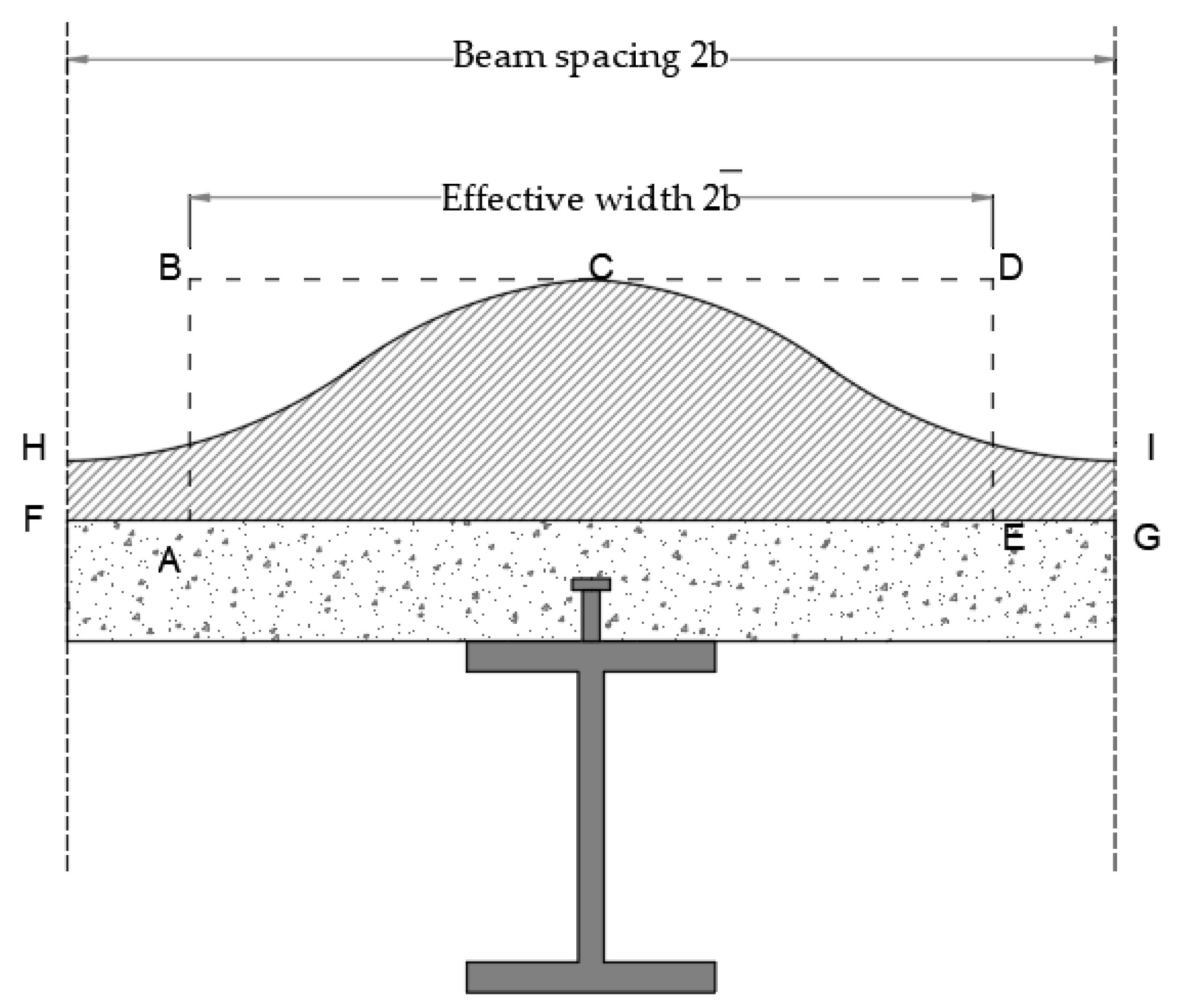
Figure 2.
Details of the beam which is named (E11).

Figure 3.
The first finite element model.

Figure 4.
The second finite element model.

Figure 5.
The MPC connectors.
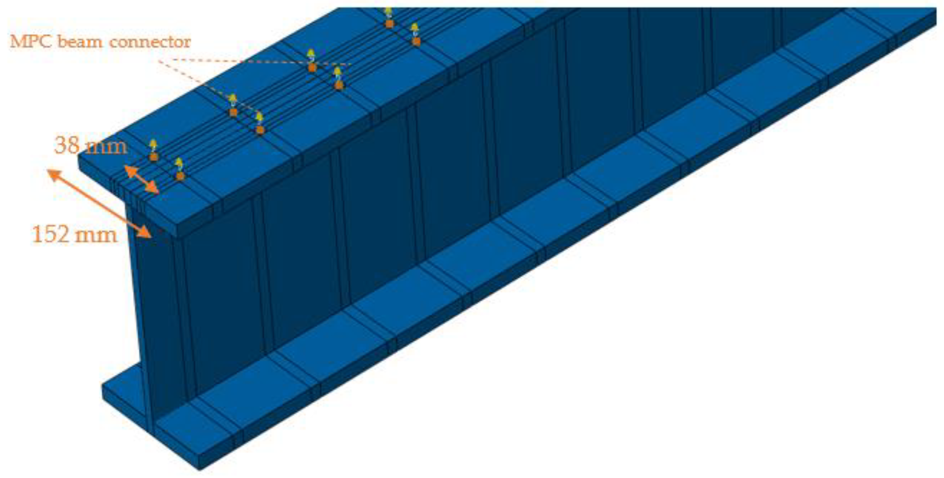
Figure 6.
The boundary conditions.
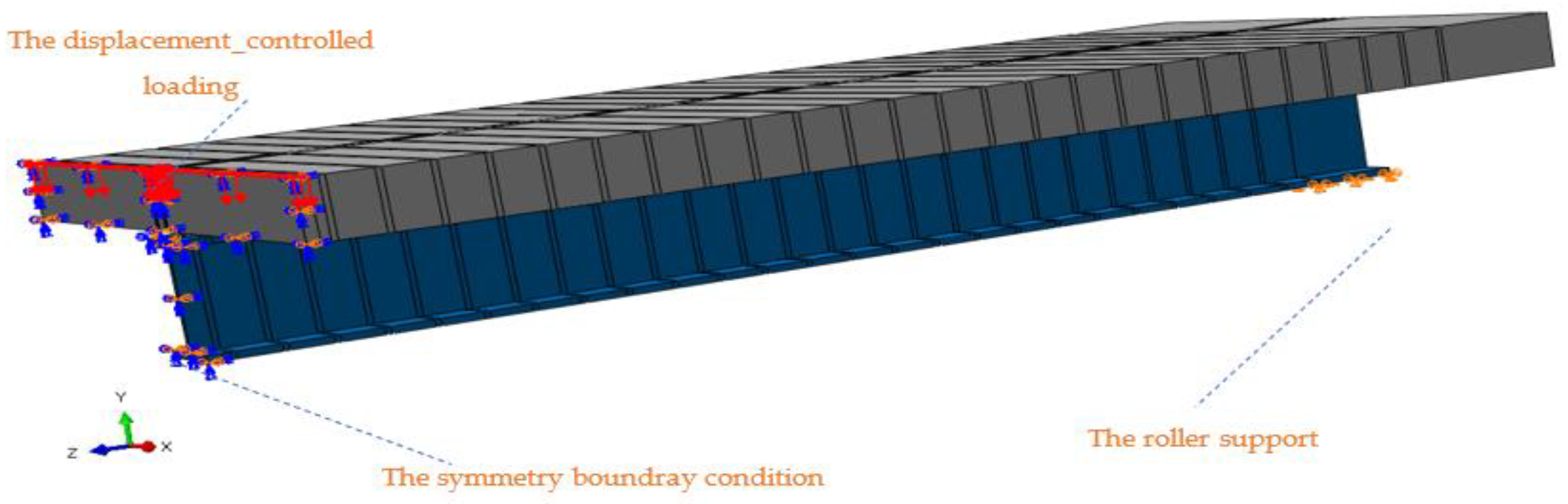
Figure 7.
The behavior of concrete under (a) uniaxial compression and (b) uniaxial tension.
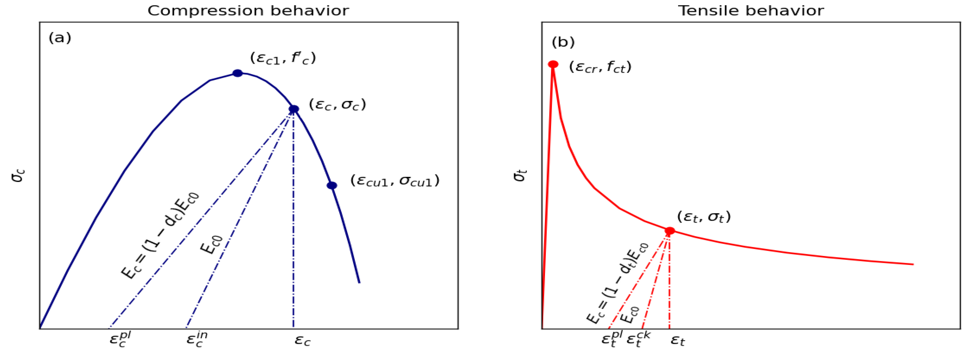
Figure 8.
Stress—inelastic strain of the concrete C50. (a) Uniaxial compression and (b) uniaxial tension.
Figure 8.
Stress—inelastic strain of the concrete C50. (a) Uniaxial compression and (b) uniaxial tension.
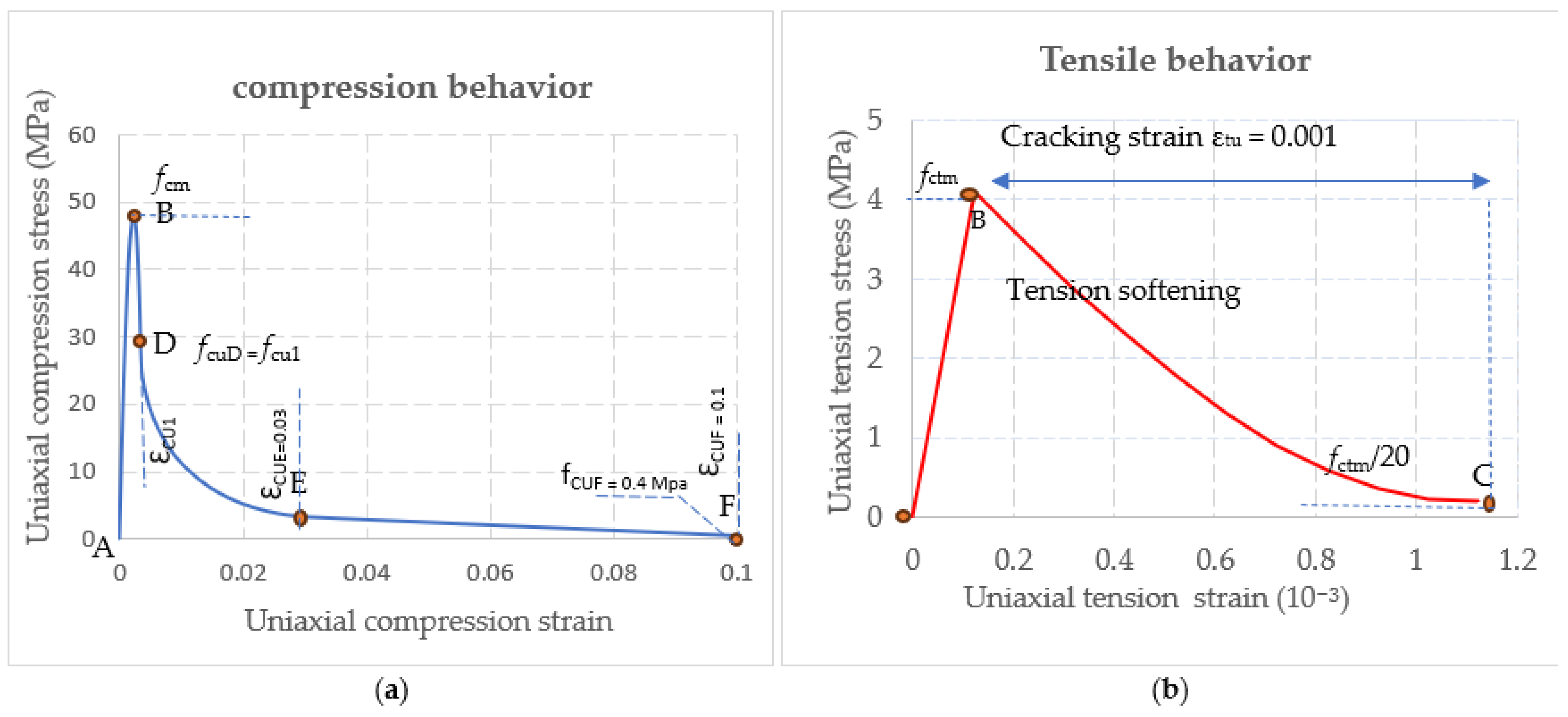
Figure 9.
Experimental and nonlinear numerical load–deflection curves for Yam and Chapman’s composite beam (E11).
Figure 9.
Experimental and nonlinear numerical load–deflection curves for Yam and Chapman’s composite beam (E11).
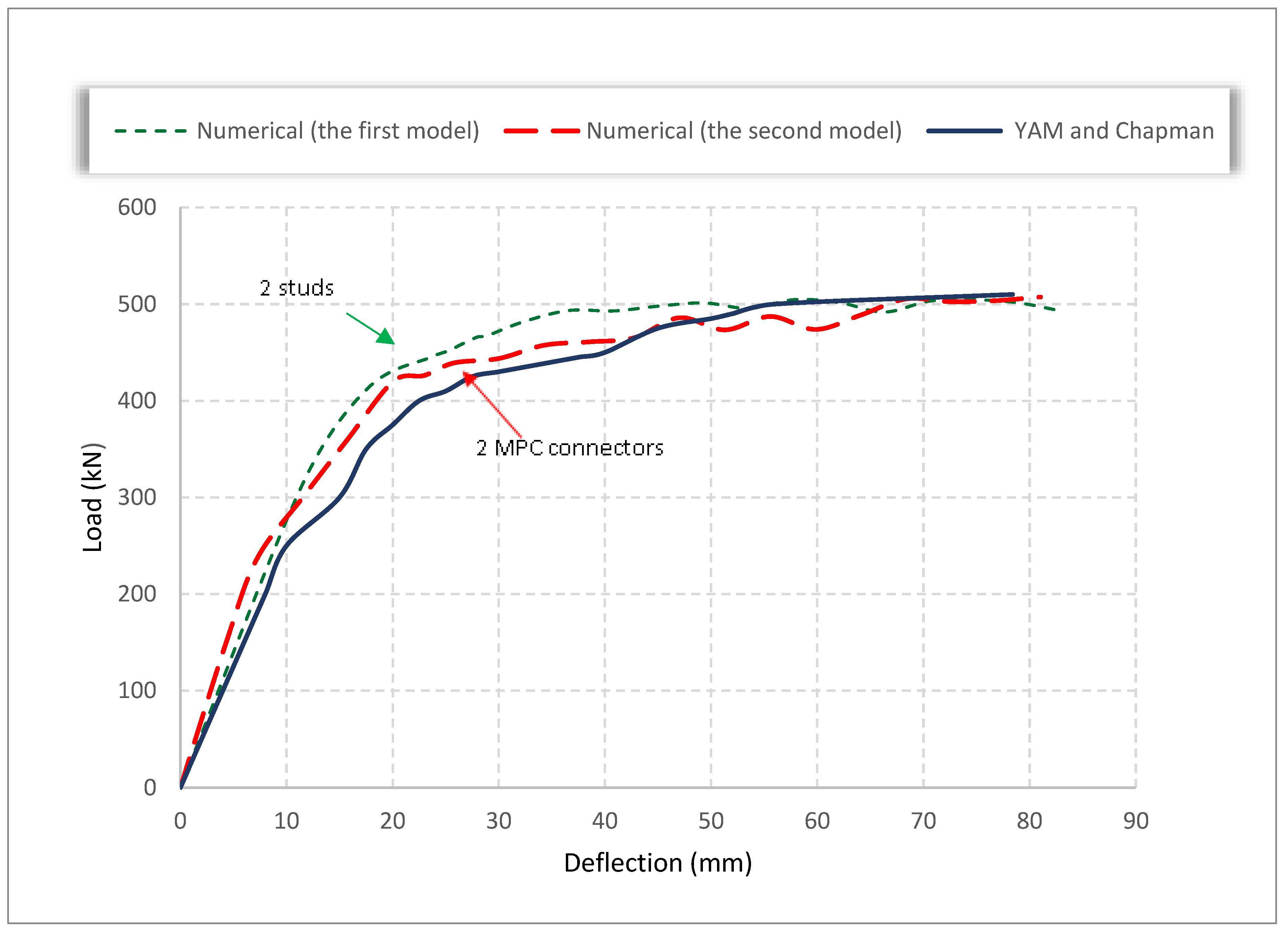
Figure 10.
Two MPC-type connector beams. (a) The surface is circular with a diameter of d = 12 mm. (b) The surface is circular with a diameter of d = 8 mm.
Figure 10.
Two MPC-type connector beams. (a) The surface is circular with a diameter of d = 12 mm. (b) The surface is circular with a diameter of d = 8 mm.
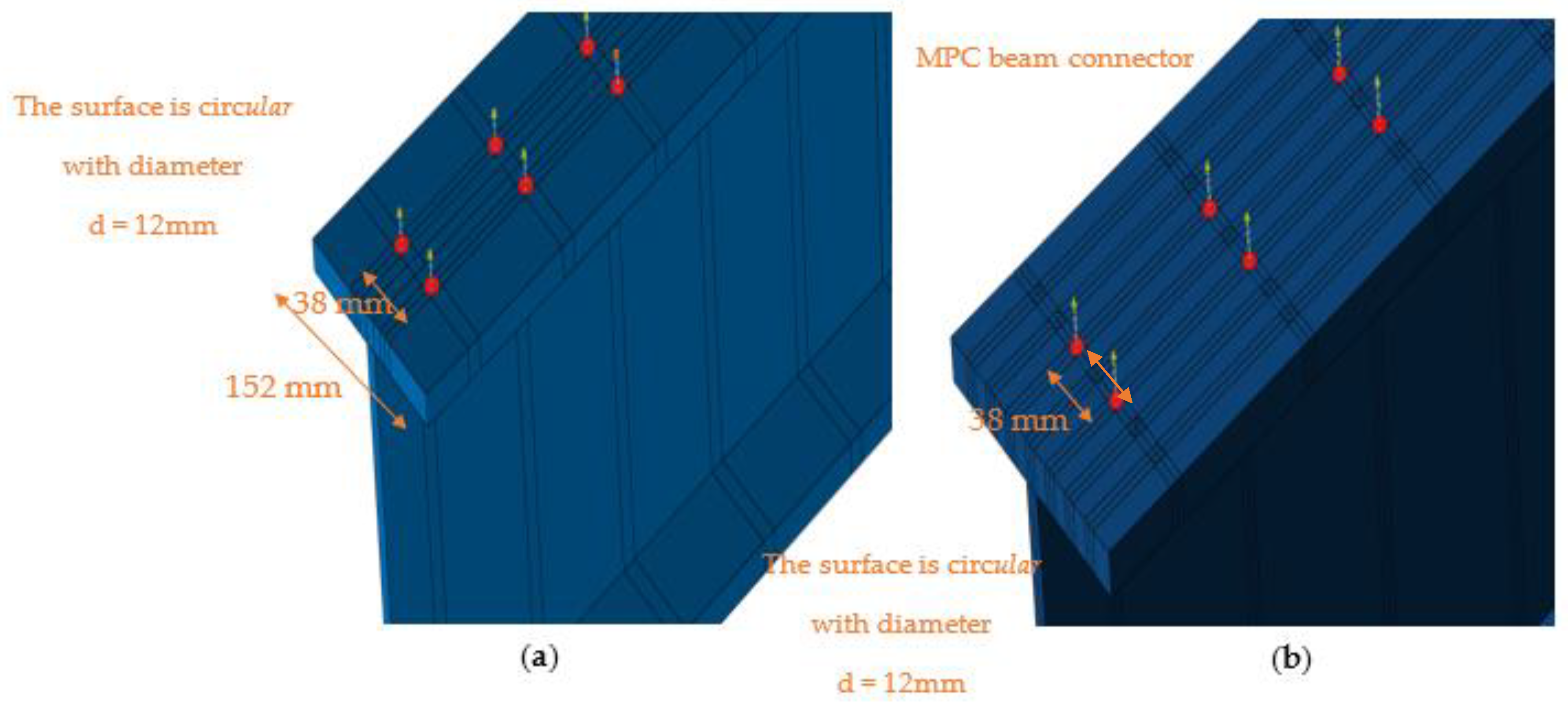
Figure 11.
Three models: (a) 2 MPC connectors, (b) 4 MPC connectors, (c) 7 MPC connectors.
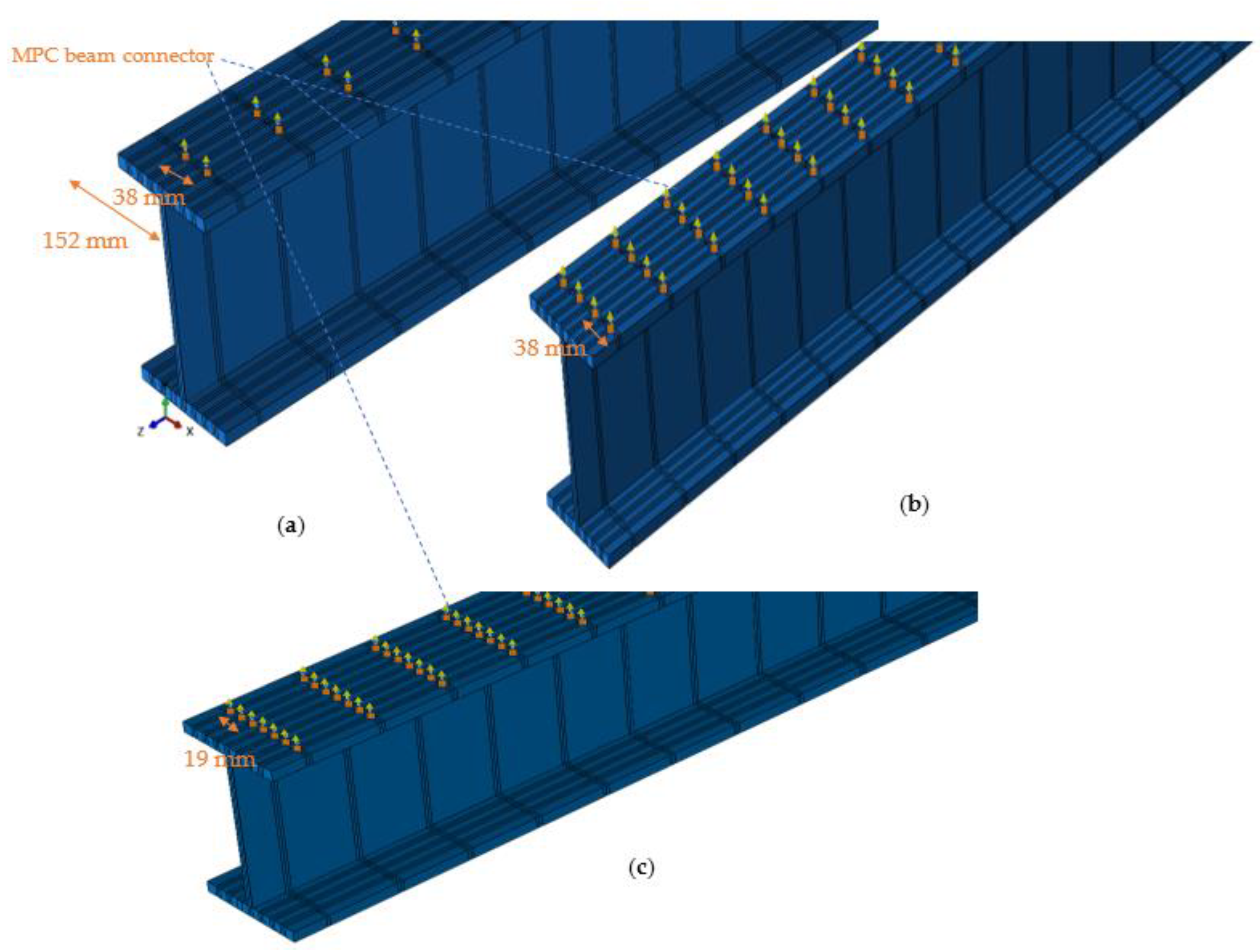
Figure 12.
The effect of the location of the shear connectors: (a) 2 MPC connectors with an a/bs ratio of 0.75, (b) 2 MPC connectors with an a/bs ratio of 0.25.
Figure 12.
The effect of the location of the shear connectors: (a) 2 MPC connectors with an a/bs ratio of 0.75, (b) 2 MPC connectors with an a/bs ratio of 0.25.
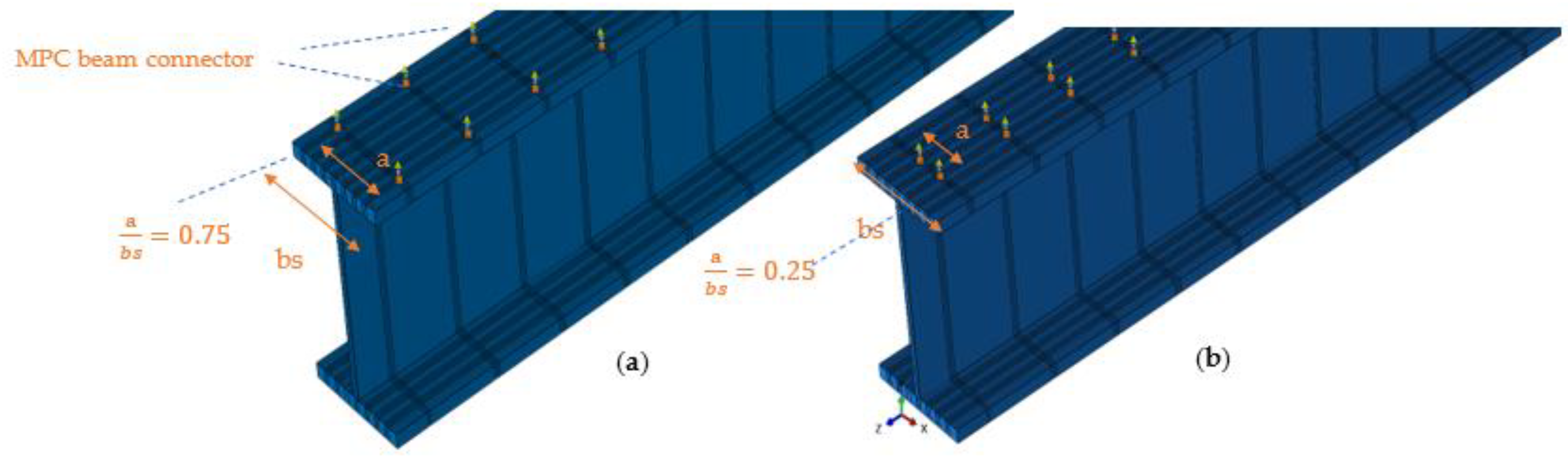
Figure 13.
The effect of the location of the shear connectors: (a) 4 MPC connectors with an a/bs ratio of 0.75, (b) 4 MPC connectors with an a/bs ratio of 0.5.
Figure 13.
The effect of the location of the shear connectors: (a) 4 MPC connectors with an a/bs ratio of 0.75, (b) 4 MPC connectors with an a/bs ratio of 0.5.

Figure 14.
The stress at the top fiber of the slab in the mid-span.
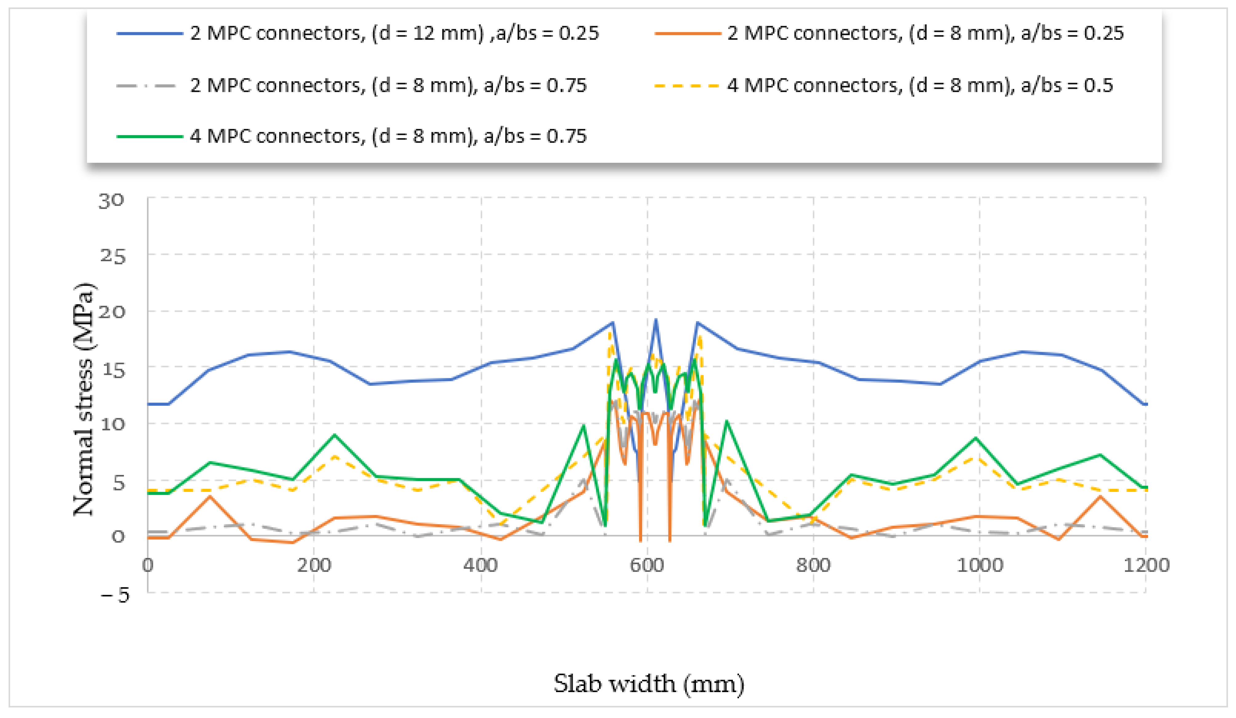
Figure 15.
The stress at the top fiber of the slab in the mid-span for (a) 7 MPC beam connector (b) 4 MPC beam conn.
Figure 15.
The stress at the top fiber of the slab in the mid-span for (a) 7 MPC beam connector (b) 4 MPC beam conn.
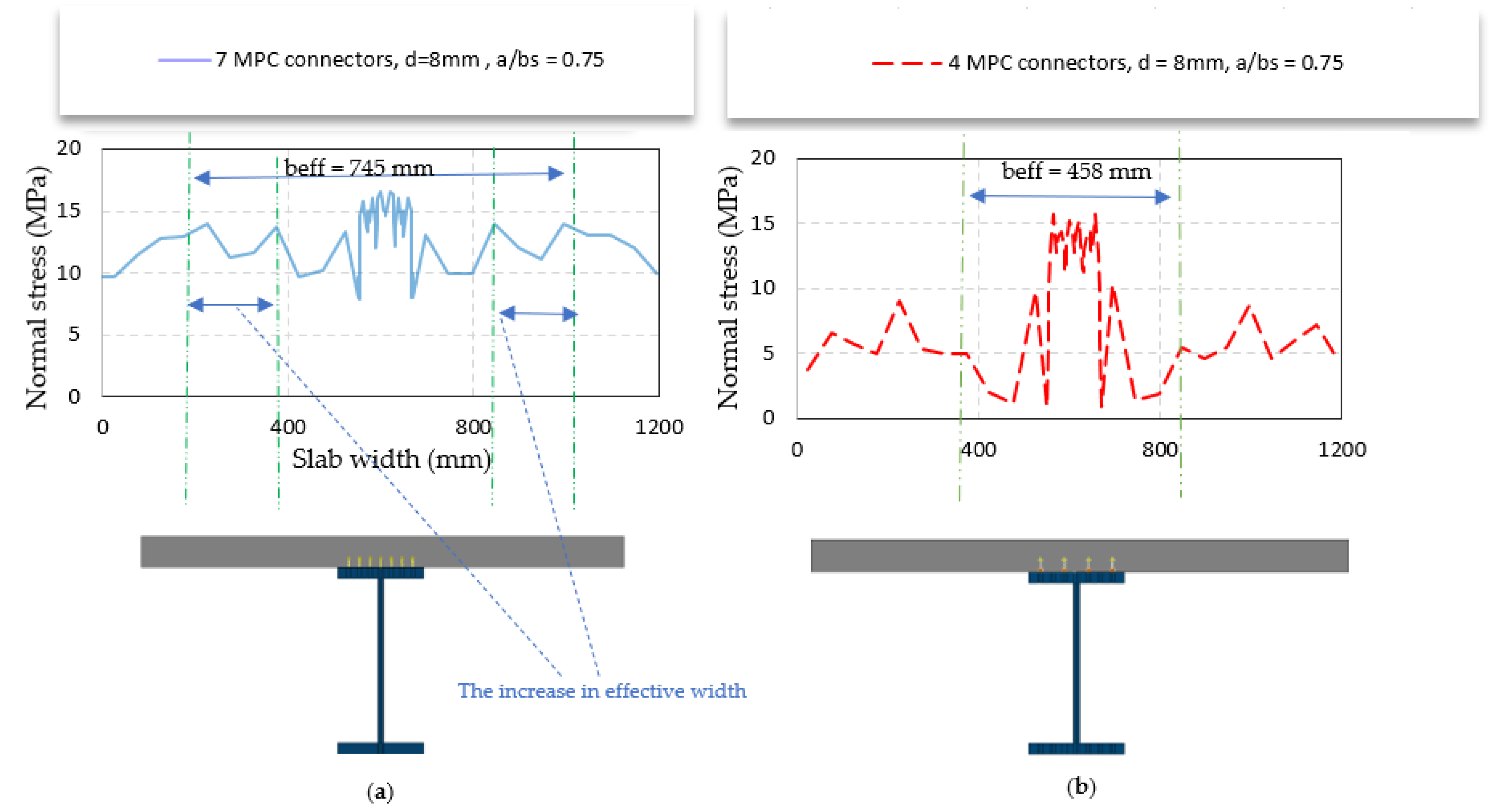
Figure 16.
The effective width along the beam span (2MPC connectors).
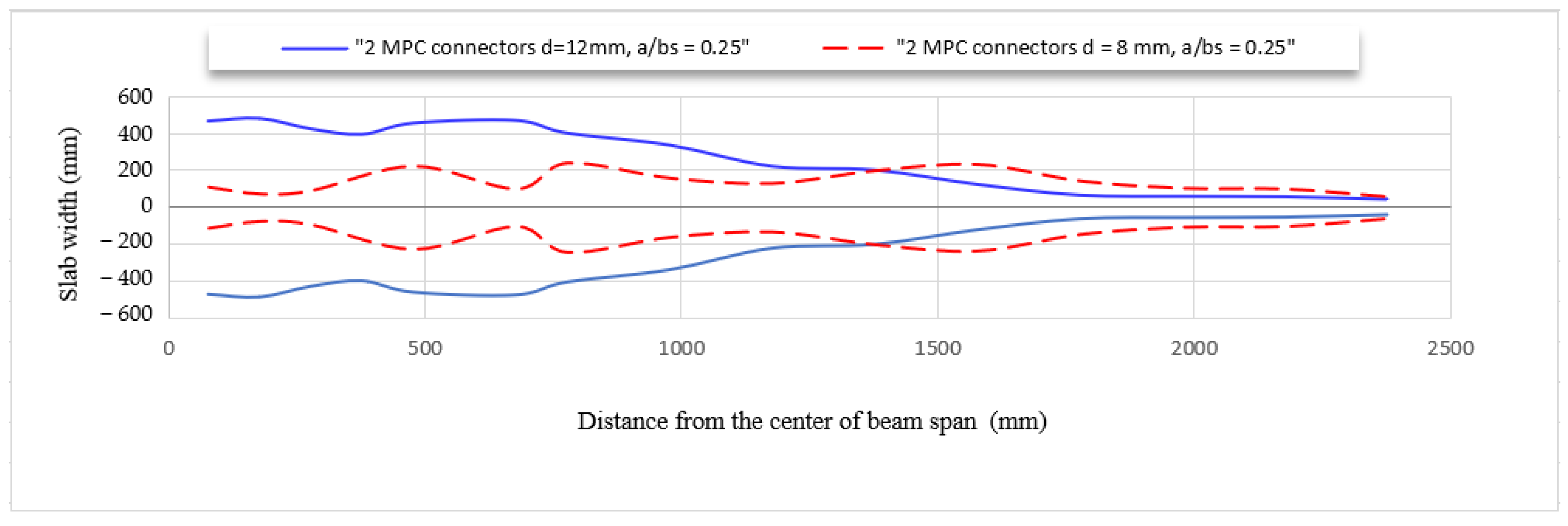
Figure 17.
The stress at the top fiber of the slab in the mid-span (2, 4, 7 MPC connectors).
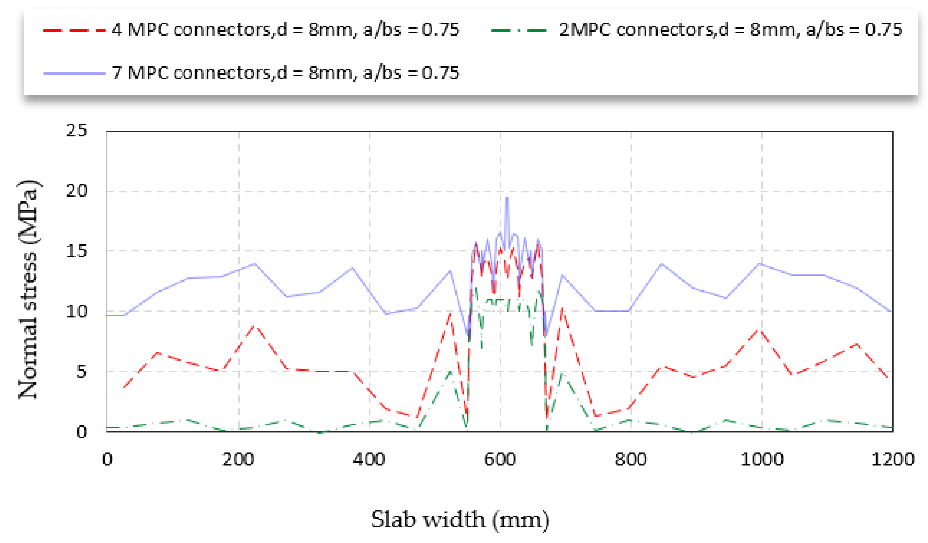
Figure 18.
The effective width along the beam span.


Table 1.
Material properties used for Yam and Chapman steel–concrete composite beam [20].
Table 1.
Material properties used for Yam and Chapman steel–concrete composite beam [20].
| Material | Symbol | Definition | Value |
|---|---|---|---|
| Concrete | f′c | Compressive (MPa) | 50 |
| Ec0 | Young’s modulus (MPa) | 33,234 | |
| fct | Tensile strength (MPa) | 4 | |
| υ | Poisson’s ratio | 0.15 | |
| Reinforcement | fy | Yield stress (MPa) | 265 (Φ16) |
| 265 (Φ12) | |||
| Es | Young’s modulus (MPa) | 205,000 | |
| υ | Poisson’s ratio | 0.3 | |
| Steel beam | fy | Yield stress (MPa) | 265 |
| υ | Young’s modulus (MPa) | 205,000 | |
| Shear connector | H | Overall length (mm) | 50 |
| φ | Diameter (mm) | 12 | |
| S stud | Spacing (mm) | 100 | |
| Es | Young’s modulus (MPa) | 205,000 |
Table 2.
CDP parameters.
| Dilation | Eccentricity | fb0/fc0 | k | Viscosity |
|---|---|---|---|---|
| 36 | 0.1 | 1.2 | 0.59 | 0 |
Table 3.
Comparison between the experimental and numerical results of Yam and Chapman’s composite beam (E11).
Table 3.
Comparison between the experimental and numerical results of Yam and Chapman’s composite beam (E11).
| Experimental [16] | Numerical (1) | Numerical (2) | Error 1% | Error 2% | |||
|---|---|---|---|---|---|---|---|
| Max. Central Deflection (mm) | 78.4 | 82.2 | 81.0 | 1.05 | 1.033 | 4.5 | 3.4 |
| Ultimate Load (kN) | 510.0 | 505 | 507.3 | 0.99 | 0.994 | 0.98 | 0.5 |
Table 4.
Analyzed models for parametric study.
| d (mm) | Number of MPC | a/bs | |
|---|---|---|---|
| Model 1 | 12 | 2 | 0.25 |
| Model 2 | 8 | 2 | 0.25 |
| Model 3 | 8 | 2 | 0.75 |
| Model 4 | 8 | 4 | 0.50 |
| Model 5 | 8 | 4 | 0.75 |
| Model 6 | 8 | 7 | 0.75 |
Disclaimer/Publisher’s Note: The statements, opinions and data contained in all publications are solely those of the individual author(s) and contributor(s) and not of MDPI and/or the editor(s). MDPI and/or the editor(s) disclaim responsibility for any injury to people or property resulting from any ideas, methods, instructions or products referred to in the content. |
© 2024 by the authors. Licensee MDPI, Basel, Switzerland. This article is an open access article distributed under the terms and conditions of the Creative Commons Attribution (CC BY) license (https://creativecommons.org/licenses/by/4.0/).
Share and Cite
MDPI and ACS Style
Hasan, A.; Subh, M.; Wardeh, G. The Concrete Effective Width of a Composite I Girder with Numerous Contact Points as Shear Connectors. Appl. Mech. 2024, 5, 163-179. https://doi.org/10.3390/applmech5010011
AMA Style
Hasan A, Subh M, Wardeh G. The Concrete Effective Width of a Composite I Girder with Numerous Contact Points as Shear Connectors. Applied Mechanics. 2024; 5(1):163-179. https://doi.org/10.3390/applmech5010011
Chicago/Turabian StyleHasan, Alaa, Moaid Subh, and George Wardeh. 2024. "The Concrete Effective Width of a Composite I Girder with Numerous Contact Points as Shear Connectors" Applied Mechanics 5, no. 1: 163-179. https://doi.org/10.3390/applmech5010011