New Analytical Expressions of Concentrations in Packed Bed Immobilized-Cell Electrochemical Photobioreactor

Abstract

An electrochemical photobioreactor with a packed bed containing transparent gel granules and immobilized photosynthetic bacterial cells is shown with a one-dimensional two-phase flow and transport model. We consider the biological/chemical events in the electrochemical photobioreactor, the intrinsically connected two-phase flow and mass transport, and other factors. This model is based on a system of nonlinear equations. This paper applies Akbari-Ganji’s and Taylor series methods to find analytical solutions to nonlinear differential equations that arise in an immobilized-cell electrochemical photobioreactor. Approximate analytical expressions of the concentration of glucose and hydrogen are obtained in liquid and gas phases for different parameter values. Numerical simulations are presented to validate the theoretical investigations.

1. Introduction

The packed bed reactor can apply to various processes, including adsorption, leaching, ion exchange, and catalysis. Consequently, over the past ten years, one of the leading research areas in chemical engineering has been mass transfer in packed beds. However, only a few mass transfer studies have been made using electrochemical techniques. Hanratty [1,2,3,4,5,6] developed an electrochemical technique to study the mass transfer phenomena in packed bed reactors. Mass transport, two-phase flow, and biological reactions interact in an active photobioreactor. Therefore, a greater understanding of the complex transport mechanism will encourage the use of photobioreactors.

Immobilized-cell bioreactors have been the subject of several mathematical models research [7,8,9,10]. Nath and Chand’s [8] research looked at the steady-state mass transfer in conjunction with the biological reaction in immobilized-cell-packed bed reactors. Using Pseudomonas putida immobilized in calcium alginate beads, Banerjee et al. [9] provided a mathematical model to analyze the mass transfer constraints in phenol biodegradation. In addition, Palazzi et al. [11] developed a kinetic model in a continuous bioreactor for hydrogen production. They studied the effect of residence time and inlet glucose concentration on the hydrogen production rate. Liao et al. [12] present a one-dimensional two-phase flow and transport model for a packed bed photobioreactor with transparent gel granules containing immobilized photosynthetic bacterial cells.

This communication directs our attention to the analytical and numerical methods of solving nonlinear equations in an immobilized-cell photobioreactor. We use Akbari-Ganji’s method (AGM) and the renowned Taylor series method (TSM) to derive approximate analytical expressions of substrate and product concentrations in liquid and gas phases for various parameter values. This paper will present a profile of both approaches’ reliability, efficiency, and convergence.

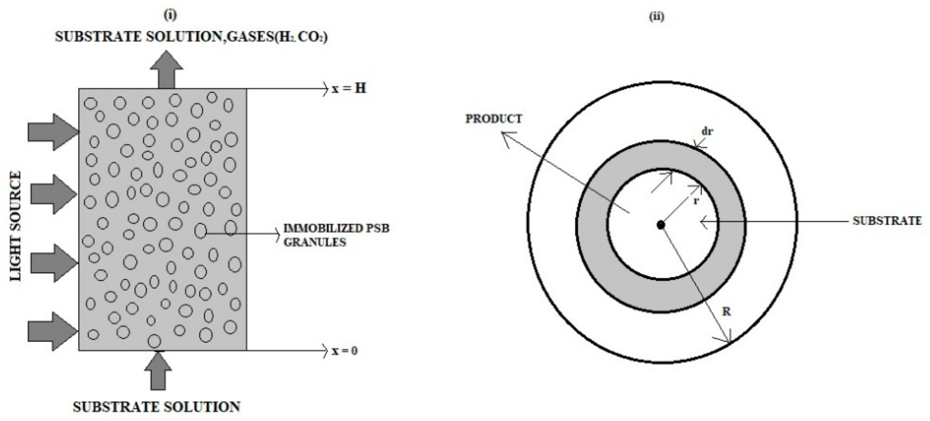
2. Formulation of the Problems

An immobilized-cell photo bioreactor packed with transparent gel-granules containing immobilized PSB developed and modeled by Shirejini et al. [13] is illustrated in Figure 1i. Figure 1ii shows a schematic diagram of mass transfer in a single gel granule, such that the mass transfer of all reactants and products is dominated by diffusion. Using Fick’s law, the mass transport equations for the substrate and the hydrogen inside the gel granules are given by [12]:

$${\mathrm{D}}_{\mathrm{granule}}^{\mathrm{S}}\left[\frac{1}{r^2}\frac{\mathrm{d}}{\mathrm{d}r}\left(r^2\frac{\mathrm{d}{\mathrm{C}}_{\mathrm{granule}}^{\mathrm{S}}}{\mathrm{d}r}\right)\right]={\varphi }_{\mathrm{granule}}^{\mathrm{S}}$$

(1)

$${\mathrm{D}}_{\mathrm{granule}}^{{\mathrm{H}}_2}\left[\frac{1}{r^2}\frac{\mathrm{d}}{\mathrm{d}r}\left(r^2\frac{\mathrm{d}{\mathrm{C}}_{\mathrm{granule}}^{{\mathrm{H}}_2}}{\mathrm{d}r}\right)\right]={\varphi }_{\mathrm{granule}}^{{\mathrm{H}}_2}$$

(2)

$${\varphi }_{\mathrm{granule}}^{\mathrm{S}}=\frac{\mu X_{\mathrm{cell}}}{Y_{X/S}^{*}}+m{X}_{\mathrm{cell}}, {\varphi }_{\mathrm{granule}}^{{\mathrm{H}}_2}=\frac{{\alpha }^{*}\mu X_{\mathrm{cell}}}{Y_{X/S}^{*}}+\beta X_{\mathrm{cell}},\mu =\frac{{ {\mu }_{\max }C}_{\mathrm{granule}}^{\mathrm{S}}}{K_{\mathrm{S}}+C_{\mathrm{granule}}^{\mathrm{S}}}$$

(3)

where ${\mathrm{D}}_{\mathrm{granule}}^{\mathrm{S}}$ and ${\mathrm{D}}_{\mathrm{granule}}^{{\mathrm{H}}_2}$ are the significant diffusion coefficients of glucose and hydrogen in the gel granule, ${\mathrm{C}}_{\mathrm{granule}}^{\mathrm{S}}$ and ${\mathrm{C}}_{\mathrm{granule}}^{{\mathrm{H}}_2}$ are the local concentrations of glucose and hydrogen inside the gel granule, ${\varphi }_{\mathrm{granule}}^{\mathrm{S}}$ is the consumption rate of glucose, ${\varphi }_{\mathrm{granule}}^{{\mathrm{H}}_2}$ is the generation rate of hydrogen. The parameter ${\alpha }^{*}$ represents the growth-associated kinetic constant for hydrogen production, $\beta$ is the non-growth-associated kinetic constant, $X_{\mathrm{cell}}$ is the initial cell density, $Y_{X/S}^{*}$ is the cell yield, and $K_{\mathrm{S}}$ is a Monod constant. Furthermore, ${\mu }_{\max }$ denotes the maximum specific growth rate, and $\mu$ is the growth rate. The boundary conditions for the above system of Equations (1) and (2) are given by

$${\left.\frac{\mathrm{d}{\mathrm{C}}_{\mathrm{granule}}^{\mathrm{S}}}{\mathrm{d}r}\right|}_{r=0}={\left.\frac{\mathrm{d}{\mathrm{C}}_{\mathrm{granule}}^{{\mathrm{H}}_2}}{\mathrm{d}r}\right|}_{r=0}=0,$$

(4)

$${\left.{\mathrm{C}}_{\mathrm{granule}}^{\mathrm{S}}\right|}_{r=R}={\mathrm{C}}_{\mathrm{l}}^{\mathrm{S}}, {\left.{\mathrm{C}}_{\mathrm{granule}}^{{\mathrm{H}}_2}\right|}_{r=R}={\mathrm{C}}_{\mathrm{g}}^{{\mathrm{H}}_2},$$

(5)

where ${\mathrm{C}}_{\mathrm{l}}^{\mathrm{S}}$ and ${\mathrm{C}}_{\mathrm{g}}^{{\mathrm{H}}_2}$ are bulk solutions, and $R$ is the radius of the catalyst. The source terms ${\phi }^s,{\phi }^{H_2}$, and ${\phi }^{C{O}_2}$ are defined by:

$${\phi }^s=\alpha D_{\mathrm{granule}}^s{\left(\frac{d{C}_{\mathrm{granule}}^s}{dr}\right)}_{r=R},{\phi }^{H_2}=\alpha D_{\mathrm{granule}}^{H_2}{\left(\frac{d{C}_{\mathrm{granule}}^{H_2}}{dr}\right)}_{r=R},$$

$${\phi }^{C{O}_2}=\frac{M^{C{O}_2}}{2M^{H_2}}{\phi }^{H_2},$$

(6)

where $\alpha$ is the specific area of the gel granule, the source terms of the liquid phase and gas phase are expressed by:

$$m_l^{•}=-{\phi }^s,m_g^{•}={\phi }^{H_2}+{\phi }^{C{O}_2}$$

(7)

Here, the dot signifies differentiation with respect to time. By introducing the dimensionless parameters

$${\mathsf{\Phi }}_1=\frac{X_{\mathrm{cell}} {\mu }_{max}{R}^2}{Y_{\frac{X}{S}}^{*} {\mathrm{D}}_{\mathrm{granule}}^{\mathrm{S}}{K}_{\mathrm{S}}}, {\mathsf{\Phi }}_2=\frac{X_{\mathrm{cell}} {\mu }_{max}{R}^2{\mathrm{C}}_{\mathrm{l}}^{\mathrm{S}}}{Y_{\frac{X}{S}}^{*} {\mathrm{D}}_{\mathrm{granule}}^{\mathrm{S}}{K}_{\mathrm{S}}{\mathrm{C}}_{\mathrm{g}}^{{\mathrm{H}}_2}},{\gamma }_1=\frac{X_{\mathrm{cell}}m R^2}{ {\mathrm{D}}_{\mathrm{granule}}^{\mathrm{S}}{K}_{\mathrm{S}}},$$

$${\gamma }_2=\frac{X_{\mathrm{cell}}m R^2}{ {\mathrm{D}}_{\mathrm{granule}}^{\mathrm{S}}{\mathrm{C}}_{\mathrm{l}}^{\mathrm{S}}},{\gamma }_3=\frac{X_{\mathrm{cell}}\beta R^2{\mathrm{C}}_{\mathrm{l}}^{\mathrm{S}}}{ {\mathrm{D}}_{\mathrm{granule}}^{\mathrm{S}}{K}_{\mathrm{S}}{\mathrm{C}}_{\mathrm{g}}^{{\mathrm{H}}_2}},{\gamma }_4=\frac{X_{\mathrm{cell}\beta }{R}^2}{ {\mathrm{D}}_{\mathrm{granule}}^{H_2}{\mathrm{C}}_{\mathrm{g}}^{{\mathrm{H}}_2}},$$

$$\zeta =\frac{r}{R}, u=\frac{C_{\mathrm{granule}}^s}{{\mathrm{C}}_{\mathrm{l}}^s}, v=\frac{C_{\mathrm{granule}}^{H_2}}{{\mathrm{C}}_{\mathrm{g}}^{H_2}} , {\alpha }_1=\frac{{\mathrm{C}}_{\mathrm{l}}^{\mathrm{S}}}{K_{\mathrm{S}}},$$

(8)

Equations (1) and (2) take the dimensionless forms:

$$\frac{1}{{\zeta }^2}\frac{d}{d\zeta }\left({\zeta }^2\frac{du(\zeta )}{d\zeta }\right)=\frac{({\phi }_1+{\gamma }_1)u(\zeta )+{\gamma }_2}{(1+{\alpha }_{1}u(\zeta ))}$$

(9)

$$\frac{1}{{\zeta }^2}\frac{d}{d\zeta }\left({\zeta }^2\frac{dv(\zeta )}{d\zeta }\right)=\frac{({\phi }_2+{\gamma }_3)u(\zeta )+{\gamma }_4}{(1+{\alpha }_{1}u(\zeta ))}$$

(10)

and the dimensionless boundary conditions are:

$$\frac{du(\zeta )}{d\zeta }=\frac{dv(\zeta )}{d\zeta }=0 \mathrm{at} \zeta =0$$

(11)

$$u\left(\zeta \right)=v\left(\zeta \right)=1 \mathrm{at} \zeta =1$$

(12)

The normalized steady-state source terms of liquid and gas phases are given by

$${\psi }_l=\frac{m_l^{•}R}{\alpha D_{\mathrm{granule}}^s{C}_l^s}=-{\left(\frac{du}{d\zeta }\right)}_{\zeta =1}$$

(13)

$${\psi }_g=\frac{m_g^{•}R}{\alpha D_{\mathrm{granule}}^{H_2}{C}_g^{H_2}}=\left(\frac{2+\omega }{2}\right){\left(\frac{dv}{d\zeta }\right)}_{\zeta =1}, \mathrm{where} \omega =\frac{M^{C{O}_2}}{M^{H_2}}.$$

(14)

3. Analytical Expression of the Concentrations Using Akbari-Ganji’s Method

Nonlinear systems of equations usually have real-world physical applications. The search for effective and reliable analytical asymptotic techniques to solve complex systems has increased over the past three decades. The following methods have received significant attention: the perturbation method (PM) [13], homotopy perturbation method (HPM) [14,15], variation iteration method (VIM) [16,17], homotopy analysis method (HAM) [18,19], differential transform method (DTM) [20,21], and Adomian decomposition method (ADM) [22], Taylor series method [23,24,25] and Akbari-Ganji’s method [26,27,28,29].

In this section, we use AGM to derive explicit expressions for the concentrations of glucose and hydrogen. The AGM is a semi-analytical approach that has shown efficacy in solving nonlinear equations [26,27,28,29]. The AGM procedure begins by assuming a solution function with unknown constant coefficients, determined by solving a system of algebraic equations constructed from the differential equations and the initial conditions.

3.1. Concentration of Glucose (Substrate)

Assume that the solution of Equation (9) is given by:

$$u(\zeta )=a_0+a_1\zeta +a_2{\zeta }^2,$$

(15)

where $a_0, a_1, \mathrm{and} a_2$ are constants. The boundary conditions (11) and (12) imply

$$a_0+a_1+a_2=1 \mathrm{and} a_1=0.$$

(16)

Now define the function $F$ as follows:

$$F(\zeta ): \frac{1}{{\zeta }^2}\frac{d}{d\zeta }\left({\zeta }^2\frac{du(\zeta )}{d\zeta }\right)-\frac{({\phi }_1+{\gamma }_1)u(\zeta )+{\gamma }_2}{(1+{\alpha }_{1}u(\zeta ))}=0$$

(17)

Then

$$F(\zeta =1): 2a_1+6a_2-\frac{({\phi }_1+{\gamma }_1)(a_0+a_1+a_2)+{\gamma }_2}{(1+{\alpha }_1(a_0+a_1+a_2))}=0.$$

(18)

Using Equation (16) in Equation (18), we have

$$a_2=\frac{{\phi }_1+{\gamma }_1+{\gamma }_2}{6(1+{\alpha }_1)},{ a}_0=1-\frac{{\phi }_1+{\gamma }_1+{\gamma }_2}{6(1+{\alpha }_1)}.$$

(19)

By substituting Equations (16) and (18) into Equation (15), the analytical expression for the substrate becomes:

$$u(\zeta )=1+\frac{{\phi }_1+{\gamma }_1+{\gamma }_2}{6(1+{\alpha }_1)}({\zeta }^2-1).$$

(20)

3.2. Concentration of Hydrogen (Product)

Similar to Equation (15), we assume that the solution to Equation (10) has the form:

$$v(\zeta )=b_0+b_1\zeta +b_2{\zeta }^2.$$

(21)

From boundary conditions (11) and (12), we obtain:

$$1=b_0+b_1+b_2, \mathrm{and} b_1=0.$$

(22)

Define the G function by

$$G\left(\zeta \right): \frac{1}{{\zeta }^2}\frac{d}{d\zeta }\left({\zeta }^2\frac{dv(\zeta )}{d\zeta }\right)-\frac{({\phi }_2+{\gamma }_3)u(\zeta )+{\gamma }_4}{(1+{\alpha }_{1}u(\zeta ))}=0,$$

(23)

Then

$$G\left(\zeta =1\right): 2b_1+6b_2-\frac{({\phi }_2+{\gamma }_3)(a_0+a_1+a_2)+{\gamma }_4}{(1+{\alpha }_1(a_0+a_1+a_2))}=0,$$

(24)

Substituting Equation (22) into Equation (24) leads to

$$b_2=\frac{{\phi }_2+{\gamma }_3+{\gamma }_4}{6(1+{\alpha }_1)}, b_0=1-\frac{{\phi }_2+{\gamma }_3+{\gamma }_4}{6(1+{\alpha }_1)},$$

(25)

and substituting Equations (22) and (25) into Equation (16), the analytical expression for the product is

$$v(\zeta )=1+\frac{{\phi }_2+{\gamma }_3+{\gamma }_4}{6(1+{\alpha }_1)}({\zeta }^2-1).$$

(26)

3.3. Normalized Steady-State Source Terms of Liquid and Gas Phases

The analytical expressions of normalized steady-state source terms of liquid and gas phases are given by:

$${\psi }_l=-\frac{\left({\phi }_1+{\gamma }_1+{\gamma }_2\right)}{3(1+{\alpha }_1)},$$

(27)

$${\psi }_g=\frac{(2+\omega )}{2}\left(\frac{\left({\phi }_2+{\gamma }_3+{\gamma }_4\right)}{3(1+{\alpha }_1)}\right).$$

(28)

The analytical expressions given by Equations (20) and (26) for the concentrations of glucose and hydrogen, respectively, are identical to the expressions obtained by the homotopy perturbation method [15].

4. Analytical Expression of the Concentrations Using Taylor Series Method

The three-century-old Taylor series method (TSM) has been recently revived and exploited to accurately and efficiently solve many nonlinear differential equations representing nonlinear models in various sciences and engineering applications [23,24,25]. In this section, we employ TSM to find the concentration of glucose (substrate) and hydrogen (product).

4.1. Concentration of Glucose (Substrate)

First, we assume that

$$u(0)=m,$$

(29)

where $m$ is an unknown constant to be determined, steady-state nonlinear reaction–diffusion equations can be written in the form:

$$\left(\zeta u^{″}(\zeta )+2u^{\prime }(\zeta )\right)\left(1+{\alpha }_{1}u(\zeta )\right)=({\phi }_1+{\gamma }_1)\zeta u(\zeta )+{\gamma }_2\zeta .$$

(30)

Taking the first three derivatives of Equation (30) with respect to $\prime \zeta \prime$ gives

$$\left(\zeta u^{‴}(\zeta )+3u^{″}(\zeta )\right)\left(1+{\alpha }_{1}u(\zeta )\right)+\left(\zeta u^{″}(\zeta )+2u^{\prime }(\zeta )\right){\alpha }_{1}u\prime (\zeta )=({\phi }_1+{\gamma }_1)\left(u(\zeta )+\zeta u^{\prime }(\zeta )\right)+{\gamma }_2,$$

(31)

$$\begin{gathered} \left(\zeta u^{⁗}\left(\zeta \right)+4u^{‴}\left(\zeta \right)\right)\left(1+{\alpha }_{1}u\left(\zeta \right)\right)+2\left(\zeta u^{‴}\left(\zeta \right)+3u^{″}\left(\zeta \right)\right){\alpha }_1{u}^{\prime }\left(\zeta \right)+ \\ \left(\zeta u^{″}\left(\zeta \right)+2u^{\prime }(\zeta )\right){\alpha }_1{u}^{″}(\zeta )=({\phi }_1+{\gamma }_1)\left(2u^{\prime }(\zeta )+\zeta u^{″}(\zeta )\right) \end{gathered}$$

(32)

$$\begin{gathered} \left(\zeta u^{\prime V}\left(\zeta \right)+5u^{⁗}\left(\zeta \right)\right)\left(1+{\alpha }_{1}u\left(\zeta \right)\right)+3\left(\zeta u^{⁗}\left(\zeta \right)+4u^{‴}\left(\zeta \right)\right){\alpha }_1{u}^{\prime }\left(\zeta \right) \\ +3\left(\zeta u^{‴}(\zeta )+3u^{″}(\zeta )\right){\alpha }_1{u}^{″}(\zeta )+\left(\zeta u^{″}(\zeta )+2u^{\prime }(\zeta )\right){\alpha }_1{u}^{‴}(\zeta )=({\phi }_1+{\gamma }_1)\left(3u^{″}(\zeta )+\zeta u^{‴}(\zeta )\right) \end{gathered}$$

(33)

For $\zeta =0$, Equations (31)–(33) give the following identities:

$$\begin{gathered} u^{″}(0)=\frac{m({\phi }_1+{\gamma }_1)+{\gamma }_2}{3({\alpha }_{1}m+1)}, u^{‴}(0)=0, u^{⁗}(0)=\frac{\left(m({\phi }_1+{\gamma }_1)+{\gamma }_2\right)\left({\phi }_1+{\gamma }_1-{\alpha }_1{\gamma }_2\right)}{5({\alpha }_{1}m+1{)}^3},u^v(0)=0 \\ {u}^{vi}(0)=\frac{\left(m({\phi }_1+{\gamma }_1)+{\gamma }_2\right)\left({\phi }_1+{\gamma }_1-{\alpha }_1{\gamma }_2\right)\left(({\phi }_1+{\gamma }_1)(3-10{\alpha }_{1}m)-13{\alpha }_1{\gamma }_2\right)}{7({\alpha }_{1}m+1{)}^5}. \end{gathered}$$

(34)

The substrate concentration, the Taylor series, is expressed by the expansion

$$u(\zeta )=u(0)+u^{\prime }(0)\frac{\zeta }{1!}+u^{″}(0)\frac{{\zeta }^2}{2!}+u^{‴}(0)\frac{3\zeta }{3!}+\dots =m+u_1\frac{{\zeta }^2}{2!}+u_2\frac{{\zeta }^4}{4!}+u_3\frac{{\zeta }^6}{6!},$$

(35)

where

$$u_1=\frac{m\left({\phi }_1+{\gamma }_1\right)+{\gamma }_2}{3\left({\alpha }_{1}m+1\right)},u_2=\frac{\left(m\left({\phi }_1+{\gamma }_1\right)+{\gamma }_2\right)\left({\phi }_1+{\gamma }_1-{\alpha }_1{\gamma }_2\right)}{5({\alpha }_{1}m+1{)}^3},$$

$$u_3=\frac{\left(m({\phi }_1+{\gamma }_1)+{\gamma }_2\right)\left({\phi }_1+{\gamma }_1-{\alpha }_1{\gamma }_2\right)\left(({\phi }_1+{\gamma }_1)(3-10{\alpha }_{1}m)-13{\alpha }_1{\gamma }_2\right)}{7({\alpha }_{1}m+1{)}^5}$$

(36)

Using the boundary conditions $\zeta =1, u\left(\zeta \right)=1$ in Equation (35) implies that

$$m+u_1\frac{1}{2!}+u_2\frac{1}{4!}+u_3\frac{1}{6!}=1,$$

(37)

from which the unknown constant m can be obtained. For the fixed values of the parameters:

${\phi }_1=5,{\gamma }_1=0.1,{\gamma }_2=0.1$ and ${\alpha }_1=5$, the numerical value of m is found to be $m=0.85803,$ and from Equation (36), we obtain $u_1=0.141015,u_2=0.001159$ and $u_3=-0.000207$, and thus, from Equation (35), we obtain the analytical expression of the concentration of glucose (substrate) expressed by

$$u(\zeta ).=0.85803+0.141015\frac{{\zeta }^2}{2!}+0.001159\frac{{\zeta }^4}{4!}-0.000207\frac{{\zeta }^6}{6!}.$$

(38)

4.2. Concentration of Hydrogen (Product)

Similar to the approach in Section 4.1, we begin by assuming that

$$v\left(0\right)=l,$$

(39)

where l is an unknown constant to be determined, and by direct differentiation of $v(\zeta )$, we obtain,

$$v^{″}(0)=\frac{m({\phi }_2+{\gamma }_3)+{\gamma }_4}{3(1+{\alpha }_{1}m)}, v^{‴}(0)=0 ,v^{⁗}(0)=\frac{\left(m({\phi }_1+{\gamma }_1)+{\gamma }_2\right)\left({\phi }_2+{\gamma }_3-{\alpha }_1{\gamma }_4\right)}{5(1+{\alpha }_{1}m{)}^3}, v^v(0)=0,$$

$$v^{vi}(0)=\frac{\left(m({\phi }_{‘1}+{\gamma }_1)+{\gamma }_2\right)\left({\phi }_2+{\gamma }_3-{\alpha }_1{\gamma }_4\right)\left(({\phi }_1+{\gamma }_1)(1-{\alpha }_{1}m)-2{\alpha }_1{\gamma }_2\right)}{7(1+{\alpha }_{1}m{)}^5}.$$

(40)

Now, the product concentration is readily obtained using the Taylor series as follows:

$$v\left(\zeta \right)=v\left(0\right)+v^{\prime }\left(0\right)\frac{\zeta }{1!}+v^{″}\left(0\right)\frac{{\zeta }^2}{2!}+v^{‴}\left(0\right)\frac{{\zeta }^3}{3!}+\dots ,$$

(41)

Using the boundary condition, $v\left(1\right)=1,$ in Equation (41), gives the numerical value of $l$. For the fixed values of the parameters ${\phi }_1=1,{ \gamma }_1=1,{ \gamma }_2=1, {\phi }_2=5,{ \gamma }_3=0.1,{ \gamma }_4=0.1, {\alpha }_1=5$ and $m=0.915769$, we obtain $l=0.8563317$. The analytical expression for the product concentration takes on the form

$$v(\zeta )=0.8563317+0.1425122\frac{{\zeta }^2}{2!}+0.0011589\frac{{\zeta }^4}{4!}-0.0000581\frac{{\zeta }^6}{6!}$$

(42)

4.3. Normalized Steady-State Source Terms of Liquid and Gas Phases

The analytical expression of the normalized steady-state source terms of liquid phases (${\psi }_l)$ is obtained from the Equation,

$$-{\psi }_l=u_1+u_2\frac{1}{6}+u_3\frac{1}{120}.$$

(43)

When using the values $u_1=0.141015,u_2=0.001159$, and $u_3=-0.000207$, we obtain $-{\psi }_l=0.141207$. The analytical expression of normalized steady-state terms of gas phases, ${\psi }_g$, is given by

$${\psi }_g=\frac{2+\omega }{2}\left[v_1+v_2\frac{1}{6}+v_3\frac{1}{120}\right],$$

(44)

where ${\psi }_g=0.214057$ when $\omega =1.$

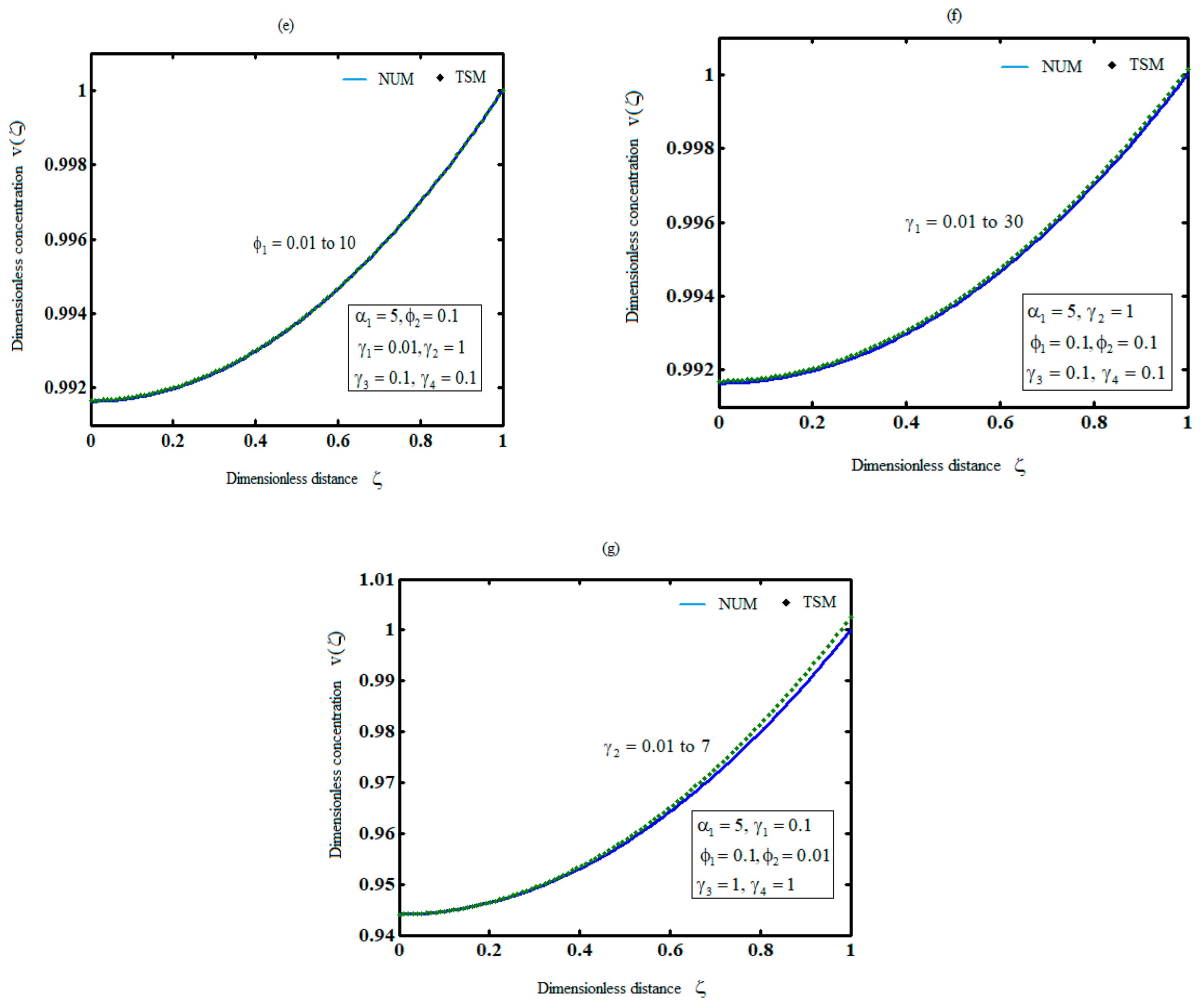
5. Comparison of Analytical Results with Previous Analytical Results and Numerical Simulation

According to Shirejini’s study [15], the homotopy perturbation approach and Praveen et al. [30] Adomian decomposition method can be utilized to successfully solve the nonlinear Equations (9) and (10). The analytical expression obtained by Shirejini et al. [15] using the HPM method or Praveen et al. [30] using the ADM method and the analytical result reported in this paper utilizing AGM are both identical as shown in Tables S1–S8 in the Supplementary Information. For large values of the parameter, HPM, ADM, and AGM don’t necessarily produce a continuous family of solutions. However, depending on the number of terms included, Taylor’s series method enables remarkably precise approximations of a function. As a result, we use the Taylor series approach to directly address the issue in our work. As previously stated, the technique described in studies [23,24,25] demonstrates the accuracy of our computations.

To examine the accuracy of the two proposed analytical approaches, we compared their results with numerical results obtained by implementing the MATLAB pdex1 function (Appendix A) and the analytical results of other methods available in the literature. The approximate analytical and numerical concentrations of substrate and product for various parameters are summarized in Tables S1–S6. Even though both methods gave satisfactory results, TSM is notably more accurate. The Table shows that the maximum relative average error is 0.6% for the TSM and 5% for the AGM. Comparisons of normalized steady-state source terms of both liquid and gas phases for various values of parameters ${\phi }_1,{\phi }_2$ and ${\alpha }_1$ are given in Tables S7 and S8.

6. Discussion

Nonlinear equations in the immobilized-cell photobioreactor are analytically solved. The Taylor series and Akbari-Ganji methods are used to get close analytical expressions of the concentrations of glucose and hydrogen inside the gel and granule. The homotopy perturbation method [12] and Adomian decomposition method [30] solved the reaction-diffusion equations representing the packed bed photobioreactor with immobilized cells [Interestingly, the semi-analytical expressions of the concentrations of substrate and product obtained using the HPM, ADM, and AGM were identical for all values of parameters.

The steady-state normalized substrate and product concentration profiles in the spherical gel granule are shown in Figure 2 and Figure 3 as functions of reaction-diffusion parameters. ${\phi }_1,{\phi }_{2,}$ ${\gamma }_1, {\gamma }_2$, ${\gamma }_3, { \gamma }_4,$ and saturation parameter ${\alpha }_1$ respectively. The mass transfer in gel granules depends on both diffusion and kinetics so that the reaction-diffusion parameters ${\phi }_1,{\phi }_2$ described the competition between diffusion and reaction in the spherical gel granule. Reaction-diffusion parameters depend upon the radius of the gel-granule R, cell density X_cell, the maximum specific growth rate m_max, diffusion coefficient of substrate Ds granule, and Monod constant Ks (refer Equation (8)).

When ${\phi }_1,{\phi }_2$ possess small values, both diffusion of substrate and product are faster than the biochemical reaction that the overall uptake of the substrate in the gel-granule is controlled by kinetic. Under these conditions, the substrate and product normalized concentration profiles across the gel granule are uniform. When the reaction-diffusion parameters are large, diffusion limitations are the principal determining factors. In addition, the saturation parameter ${\alpha }_1$ is an index quantifying the saturation degree of the reaction kinetics, which describes the ratio of the substrate concentration within the gel granule to the Monod constant.

From Figure 2a–c, it is evident that when ${\phi }_1$, ${\gamma }_1$ and ${\gamma }_2$ possess small values (<<0.1), the substrate concentration does not change significantly with radial direction. This is generally because, in such circumstances, the substrate diffusion rate is substantially larger than the rate of the biodegradation reaction. As a result, the gel granules mixing action improves, and the substrate concentration there is about uniform. In addition, Figure 2d shows that the substrate concentration dropped as the saturation value increased, indicating that more substrate was utilized. Also, from Equation (20), it is observed that the concentration substrate reaches the minimum value of $1-\frac{{\phi }_1+{\gamma }_1+{\gamma }_2}{6(1+{\alpha }_1)}$ at $\zeta =0$.

Figure 3a–g displays the normalized product concentration, v, along the radial direction. Comparing Figure 3a–d, it can be concluded that decreasing the value of ${\phi }_{2,}{\gamma }_2$, ${\gamma }_4$ and increasing the saturation parameter ${\alpha }_1$ results in high values of product concentration. From Figure 3e–g, it is observed that there is no significant difference in substrate concentration for the parameter ${\phi }_1$, ${\gamma }_1$, and ${\gamma }_2$. Additionally, it can be seen from Equation (26) that the concentration product approaches the minimal value $1-\frac{{\phi }_2+{\gamma }_3+{\gamma }_4}{6(1+{\alpha }_1)}$ at $\zeta =0$.

Table S7 illustrates the source term profile of the liquid phase for various values of ${\phi }_1$ ${\phi }_2$ and ${\alpha }_i$. From these Tables, it is seen that the values of ${\alpha }_i$ decreases and ${\phi }_1$ increases, the absolute values of the liquid phase source term increases. Table S8 represents the source term of the gas phase. As these figures reveal, it can be seen that the value of the source term in the gas phase decreases as the values of ${\phi }_{2,}$ decreases and ${\alpha }_i$ increases. Therefore, it follows from Tables S7 and S8 that in order to achieve a high mass transfer rate between the gas and liquid phases, the reaction-diffusion parameter’s values should be increased while the saturation parameter’s values should be decreased.

From our analytical results, glucose consumption efficiency ($\mu )$ and hydrogen production rate (HPR) can be obtained using the following expression.

$$\mu =\left[\frac{\mathrm{glucose} \mathrm{concentration} \mathrm{at} \mathrm{the} \mathrm{inlet}-\mathrm{glucose} \mathrm{concentration} \mathrm{at} \mathrm{the} \mathrm{outlet}}{\mathrm{glucose} \mathrm{concentration} \mathrm{at} \mathrm{the} \mathrm{inlet}}\right]100$$

$$HPR=\left[\frac{\mathrm{Amount} \mathrm{of} {\mathrm{H}}_2 \mathrm{Produced}}{{(H}_2 \mathrm{evolution} \mathrm{time})(\mathrm{photobioreactor} \mathrm{volume}) }\right]$$

Employing the glucose consumption efficiency and hydrogen production rate, the immobilized-cell photobioreactor’s performance can be investigated.

7. Conclusions

The objective of this research is multi-fold. First, we successfully employed two widely used analytical methods (AGM and TSM) to solve two reaction-diffusion equations representing the packed bed photobioreactor with immobilized cells. We also derived simple semi-analytical expressions of the substrate and product concentrations in liquid and gas phases. Second, we studied the effect of the reaction-diffusion parameters on substrate and product concentrations. Third, we added helpful information to the literature about exploiting widely used methods, particularly the AGM and TSM. As both methods are effective and reliable in solving nonlinear systems, the AGM is more or less a modification of the Adomian decomposition method, and hence, it is likely to involve some tedious algebraic computations. The TSM, on the other hand, requires fewer algebraic calculations, produces more accurate solutions, and ensures convergence if Taylor theorem criteria are satisfied.

References

1. Reiss, L.P.; Hanratty, T.J. Measurement of instantaneous rates of mass transfer to a small sink on a hall. AIChE J. 1962, 8, 245–247. [Google Scholar] [CrossRef]
2. Relas, L.P.; Hanratty, T.J. An Experimental study of the unsteady nature of the viscous sublayer. AIChE J. 1963, 9, 154–160. [Google Scholar] [CrossRef]
3. Shaw, P.V.; Hanratty, T.J. Fluctuations in the local rate of turbulent mass transfer to a pipe hall. AIChE J. 1964, 10, 475–482. [Google Scholar] [CrossRef]
4. Shaw, P.V.; Reiss, L.P.; Hanratty, T.J. Rates of turbulent transfer to a pipe hall in the mass transfer entry region. AIChE J. 1963, 9, 362–364. [Google Scholar] [CrossRef]
5. Jolls, K.R.; Hanratty, T.J. Use of electrochemical techniques to study mass transfer rates and local skin friction to a sphere in a dumped bed. AIChE J. 1969, 15, 199. [Google Scholar] [CrossRef]
6. Karabelas, A.J.; Wegner, T.H.; Hanratty, T.J. Use of asymptotic relations to correlate mass transfer data in packed beds. Chem. Eng. Sci. 1971, 26, 1581–1589. [Google Scholar] [CrossRef]
7. Tepe, O.; Dursun, A.Y. Combined effects of external mass transfer and biodegradation rates on removal of phenol by immobilized Ralstonia eutropha in a packed bed reactor. J. Hazard. Mater. 2008, 151, 9–16. [Google Scholar] [CrossRef]
8. Nath, S.; Chand, S. Mass transfer and biochemical reaction in immobilized cell packed bed reactors: Correlation of experiment with theory. J. Chem. Technol. Biotechnol. 1996, 66, 286–292. [Google Scholar] [CrossRef]
9. Banerjee, I.; Modak, J.M.; Bandopadhyay, K.; Das, D.; Maiti, B.R. Mathematical model for evaluation of mass transfer limitations in phenol biodegradation by immobilized Pseudomonas putida. J. Biotechnol. 2001, 87, 211–223. [Google Scholar] [CrossRef]
10. Wang, J.L.; Wan, W. Kinetic models for fermentative hydrogen production: A review. Int. J. Hydrog. Energy 2009, 34, 3313–3323. [Google Scholar] [CrossRef]
11. Palazzi, E.; Perego, P.; Fabiano, B. Mathematical modelling and optimization of hydrogen continuous production in a fixed bed bioreactor. Chem. Eng. Sci. 2002, 57, 3819–3830. [Google Scholar] [CrossRef]
12. Liao, Q.; Liu, D.M.; Ye, D.D.; Zhu, X.; Lee, D.J. Mathematical modeling of two-phase flow and transport in an immobilized-cell photobioreactor. Int. J. Hydrog. Energy 2011, 36, 13936–13948. [Google Scholar] [CrossRef]
13. Shirejini, S.Z.; Fattahi, M. Mathematical modeling and analytical solution of two-phase flow transport in an immobilized-cell photobioreactor using the homotopy perturbation method (HPM). Int. J. Hydrog. Energy 2016, 41, 18405–18417. [Google Scholar] [CrossRef]
14. Ganji, D.; Hosseini, M.; Shayegh, J. Some nonlinear heat transfer equations solved by three approximate methods. Int. Commun. Heat Mass Transf. 2007, 34, 1003–1016. [Google Scholar] [CrossRef]
15. He, J.H. Homotopy perturbation technique. Comput. Methods Appl. Mech. Eng. 1999, 178, 257–262. [Google Scholar] [CrossRef]
16. He, J.H. Variational iteration method for autonomous ordinary differential systems. Appl. Math. Comput. 2000, 114, 115–123. [Google Scholar] [CrossRef]
17. Ghafoori, S.; Motevalli, M.; Nejad, M.G.; Shakeri, F.; Ganji, D.D.; Jalaal, M. Efficiency of differential transformation method for nonlinear oscillation: Comparison with HPM and VIM. Curr. Appl. Phys. 2011, 11, 965–971. [Google Scholar] [CrossRef]
18. Liao, S.J. The Proposed Homotopy Analysis Technique for the Solution of Nonlinear Problems. Ph.D. Thesis, Shanghai Jiao Tong University, Shanghai, China, 1992. [Google Scholar]
19. Liao, S.J. Beyond Perturbation: Introduction to Homotopy Analysis Method; Chapman & Hall/CRC: Boca Raton, FL, USA, 2003. [Google Scholar]
20. Arikoglu, A.; Ozkol, I. Solution of difference equations by using differential transform method. Appl. Math. Comput. 2006, 174, 1216–1228. [Google Scholar] [CrossRef]
21. Soltanalizadeh, B. Differential transformation method for solving one-space-dimensional telegraph equation. Comput. Appl. Math. 2011, 30, 639–653. [Google Scholar] [CrossRef]
22. Wazwaz, A.M. A reliable modification of Adomian decomposition method. Appl. Math. Comput. 1999, 102, 77–86. [Google Scholar] [CrossRef]
23. AlRasheed, N.N. Adaptation of Taylor’s Formula for Solving System of Differential Equations. Nonlinear Differ. Equ. App. 2016, 4, 95–107. [Google Scholar] [CrossRef]
24. El-Ajou, A.; Abu Arqub, O.; Al-Smadi, M. A general form of the generalized Taylor’s formula with some applications. Appl. Math. Comput. 2015, 256, 851–859. [Google Scholar] [CrossRef]
25. He, C.H.; Shen, Y.; Ji, F.Y.; He, J.H. Taylor series solution for Fractal Bratu-Type equation arising in electrospinning process. Fractals 2020, 28, 2050011. [Google Scholar] [CrossRef]
26. Akbari, M.R.; Ganji, D.D.; Nimafar, M.; Ahmadi, A.R. Significant progress in solution of nonlinear equations at displacement of structure and heat transfer extended surface by new AGM approach. Front. Mech. Eng. 2014, 9, 390–401. [Google Scholar] [CrossRef]
27. Akbari, M. Nonlinear Dynamic in Engineering by Akbari-Ganji’s Method; Xlibris Corporation: Bloomington, IN, USA, 2015. [Google Scholar]
28. Ganji, D.D.; Talarposhti, R.A. Numerical and Analytical Solutions for Solving Nonlinear Equations in Heat Transfer; Technology and Engineering, IGI Global: Hershey, PA, USA, 2017. [Google Scholar]
29. Sheikholeslami, M.; Ganji, D.D. Applications of Semi-Analytical Methods for Nanofluid Flow and Heat Transfer; Elsevier: Oxford, UK, 2018. [Google Scholar]
30. Praveen, T.; Rajendran, L. Theoretical analysis through mathematical modeling of two-phase flow transport in an immobilized-cell photobioreactor. Chem. Phys. Lett. 2015, 625, 193–201. [Google Scholar] [CrossRef]
Figure 1. Schematic of (i) a photobioreactor that contains granules of gel that have immobilised PSB cells and (ii) a single gel granule [13].
Electrochem 04 00029 g001
Figure 2. Plot of substrate concentration for various values of parameters (a) φ 2 (b) γ 1 (c) γ 2 (d) α 1 using Equations (20) and (35).
Electrochem 04 00029 g002
Figure 3. Plot of product concentration v ( ζ ) for various values of the parameters (a) ϕ 2 (b) γ 3 (c) γ 4 (d) α 1 (e)   ϕ 1 (f) γ 1 and (g) γ 2 using Equations (26) and (41).
Electrochem 04 00029 g003aElectrochem 04 00029 g003b
Disclaimer/Publisher’s Note: The statements, opinions and data contained in all publications are solely those of the individual author(s) and contributor(s) and not of MDPI and/or the editor(s). MDPI and/or the editor(s) disclaim responsibility for any injury to people or property resulting from any ideas, methods, instructions or products referred to in the content.