Article

Freshwater Invertebrate Assemblage Composition and Water Quality Assessment of an Urban Coastal Watershed in the Context of Land-Use Land-Cover and Reach-Scale Physical Habitat

by
Nicole D. Henderson
1 and
Alan D. Christian
1,2,*
1
Biology Department, University of Massachusetts Boston, Boston, MA 02125, USA
2
Honors Program, Clarkson University, Potsdam, NY 13699, USA
*
Author to whom correspondence should be addressed.
Ecologies 2022, 3(3), 376-394; https://doi.org/10.3390/ecologies3030028
Submission received: 28 April 2022 / Revised: 15 August 2022 / Accepted: 31 August 2022 / Published: 13 September 2022
(This article belongs to the Special Issue The Ecology of Rivers, Floodplains and Oxbow Lakes)

Abstract

:
Stream ecosystems provide invaluable ecosystem services but are highly impacted ecosystems in need of water quality monitoring for habitat change impacts. Freshwater macroinvertebrate (FWI) assemblages have been shown to be good indicators of water quality and are known to be vulnerable to land-use land cover (LULC) and other habitat changes. The goal of this case study was to use an existing dominant LULC analysis in the Neponset River watershed, Massachusetts, USA, as LULC sampling treatment groups to deliberately capture the influence of these LULC effects on meso-scale habitat quality, FWI assemblages, and FWI water quality indices at eight sampling reaches. To achieve this goal, we collected physical habitat measurements and FWI samples in the summers of 2010 and 2012 at eight reach-scale stations spread across four previously determined LULC sub-watershed types (forest, residential, industrial, and golf) in the watershed. We expected that LULC change would influence the habitat quality, which would influence the FWI assemblage water quality scores and composition. We also expected that the water quality at these LULC sub-watershed types would be reflected in the FWI assemblage composition. We identified five major findings from our study. Our first finding was that the habitat quality in the Neponset River watershed was somewhat degraded relative to pristine conditions. Our second finding was that our habitat characterization analysis reflected some separation of our reach-scale macrohabitat types at land-use land-cover treatment stations with some correlations with microhabitat variables. Our third finding was that the water quality base on FWI assemblages was generally degraded in reference to pristine conditions. Our fourth finding was that, contrary to our expectations, there was no significant correlation between our reach-scale EPA habitat quality scores and FWI water quality scores. Our fifth finding was that our FWI assemblage NMS showed separation of land-use land-cover sampling stations and that that low pollution-tolerant taxa dominated some of our LULC sampling treatment stations and influenced NMS groupings.

1. Introduction

While streams and rivers make up 0.006% of the Earth’s fresh water, streams and lakes provide invaluable ecosystem services and are arguably the most impacted ecosystems on the planet [1]. Freshwater ecosystems are considered some of the most impacted ecosystems on Earth with both persisting (e.g., flow modification, habitat degradation, over-exploitation, species invasion and water pollution) [2,3] and emerging threats [3]. Considering the importance and imperilment of streams, an important management action is to assess and monitor freshwater ecosystems and evaluate the associated biotic communities and their habitat.
Habitat is broadly defined as “the place or environment where a plant or animal naturally or normally lives and grows” [4]. It has been argued that habitat serves as a template on which evolution forges characteristic life-history strategies [5,6]. Stream habitats are often organized hierarchically over spatial–temporal scales ranging from larger scale catchments (stream systems), which encompass the spatially smaller and temporally shorter segment-scale (segment systems), reach-scale (reach systems), meso-scale (pool/riffle systems), and micro-scale (micro-habitat systems) units [7,8]. Furthermore, it is generally accepted that stream habitats integrate physical, chemical, and biological interactions (Barbour et al. 1999) and that habitat and biological diversity may be important [9] are highly correlated [10].
Changes in land use and land cover (LULC) are reported to be one of five global change drivers threatening terrestrial and aquatic biodiversity [11], and LULC changes are considered a major influence in stream ecosystems [1,2,12]. LULC is known to influence stream and river taxa and habitat biodiversity across anthropogenic and natural gradients and across a variety of scales [13]. The principal mechanisms that LULC is believed to influence in stream ecosystems include sedimentation, nutrient enrichment, contaminant pollution, hydrologic alteration, riparian clearing, and loss of large woody debris [13]. LULC change plays a large role in the four main proximate causes of stream ecosystem change (urbanization, industry/mining, land use/agriculture, and watercourse alteration) linking to ultimate forcing factors of ecosystem destruction, physical habitat alteration, water chemistry alteration, and direct species additions and removals [1]. Physical and chemical changes due to LULC have been shown to have effects on freshwater invertebrates (FWI), fish assemblages, and nutrients as well as the local stream habitat. For example, the presence of certain FWI and fish in streams has been used as an indicator of water quality and has been shown to relate to the land use in the watershed (i.e., catchment) [14,15,16,17]. Catchment-scale LULC change also has been shown to directly and indirectly influence the composition and condition of freshwater assemblages, habitat quality, and nutrient concentrations based on contemporary LULC and historical or legacy LULC conditions [18]. Furthermore, LULC plays an important role in our understanding of the “Urban Stream Syndrome”, in which urban streams are observed to have flashier hydrographs, elevated nutrient and contamination concentrations, altered stream morphology, and reduced taxonomic biodiversity [19,20].
Stream freshwater invertebrate (FWI) assemblage composition and structure are widely used as an indicator of environmental quality [21,22,23,24]. Meanwhile, rapid bioassessment protocols and associated metrics and indices have been developed as cost-effective scientifically valid procedures, allowing for multiple site visits in short periods of time, quick turnarounds for management decisions, easily translated results for managers and the general public, and environmentally benign procedures [25]. For example, water quality bioindicator metrics and indices (or biotic integrity measures) have been developed for FWI and fish assemblages and meso-scale habitats [14,25,26,27,28,29]. Hilsenhoff [26,27] developed one of the first biotic indices using FWI to evaluate stream water quality. Hilsenhoff’s Family Biotic Index (FBI) quantifies water quality using the composition of family-level taxonomic determinations and the pollution tolerance levels of these taxonomic groups, in which higher biotic index values indicate poorer water quality [26,27]. Karr [14,28] developed the Index of Biotic Integrity (IBI) using fish species composition and condition factor metrics in which higher total index scores indicate higher water quality. Karr’s [14,28] method was later adapted for FWI assemblages through the development of the Ohio EPA’s Invertebrate Community Index (ICI) and the United States Environmental Protetion Agency’s (USEPA) citizen science biomonitoring protocol called the Streamside Biosurvey Index (SBI) [15,30]. One benefit of the EPA’s SBI is that the SBI only requires family-level taxonomic determination for most groups and that the SBI uses a simpler mathematical calculation using the rare, common, and dominant classifications and incorporating these taxonomic abundance classifications with general pollution tolerance categories [30]. Furthermore, meso-scale habitat quality assessments have been developed using a variety of meso-scale stream characteristics such as, but not limited to, abundance of reach-scale macrohabitats (e.g., riffle, run, pools, glides), instream cover, riparian zone condition, micro-habitat development, substrate composition/embeddedness, gradient, etc. [25,29].
The goal of this case study was to use an existing dominant LULC analysis in the Neponset River watershed, Massachusetts [31], as LULC sampling treatment groups to deliberately capture the influence of these LULC effects on meso-scale habitat quality, FWI assemblages, and FWI water quality indices at eight sampling reaches in Neponset River watershed. To achieve this goal, we had three objectives. Our first objective was to characterize and assess reach-scale habitat and habitat quality at eight treatment reaches using standard protocols. Our second objective was to characterize and assess FWI assemblages and water quality at eight treatment reaches using standard protocols. Our third objective was to evaluate whether there was a positive correlation between habitat quality and FWI water quality indices at the eight treatment reaches. We had two expectations associated with our study. First, we expected that habitat and FWI water quality will be degraded in the Neponset River watershed due to LULC changes from pristine land cover conditions. Second, we expected that due to differences in LULC at our eight sampling reaches that FWI assemblages at our eight sampling reaches will cluster together based on LULC treatments and the different cluster assemblages will represent assemblages tolerant of the catchment and meso-scale habitat conditions at the reaches.

2. Materials and Methods

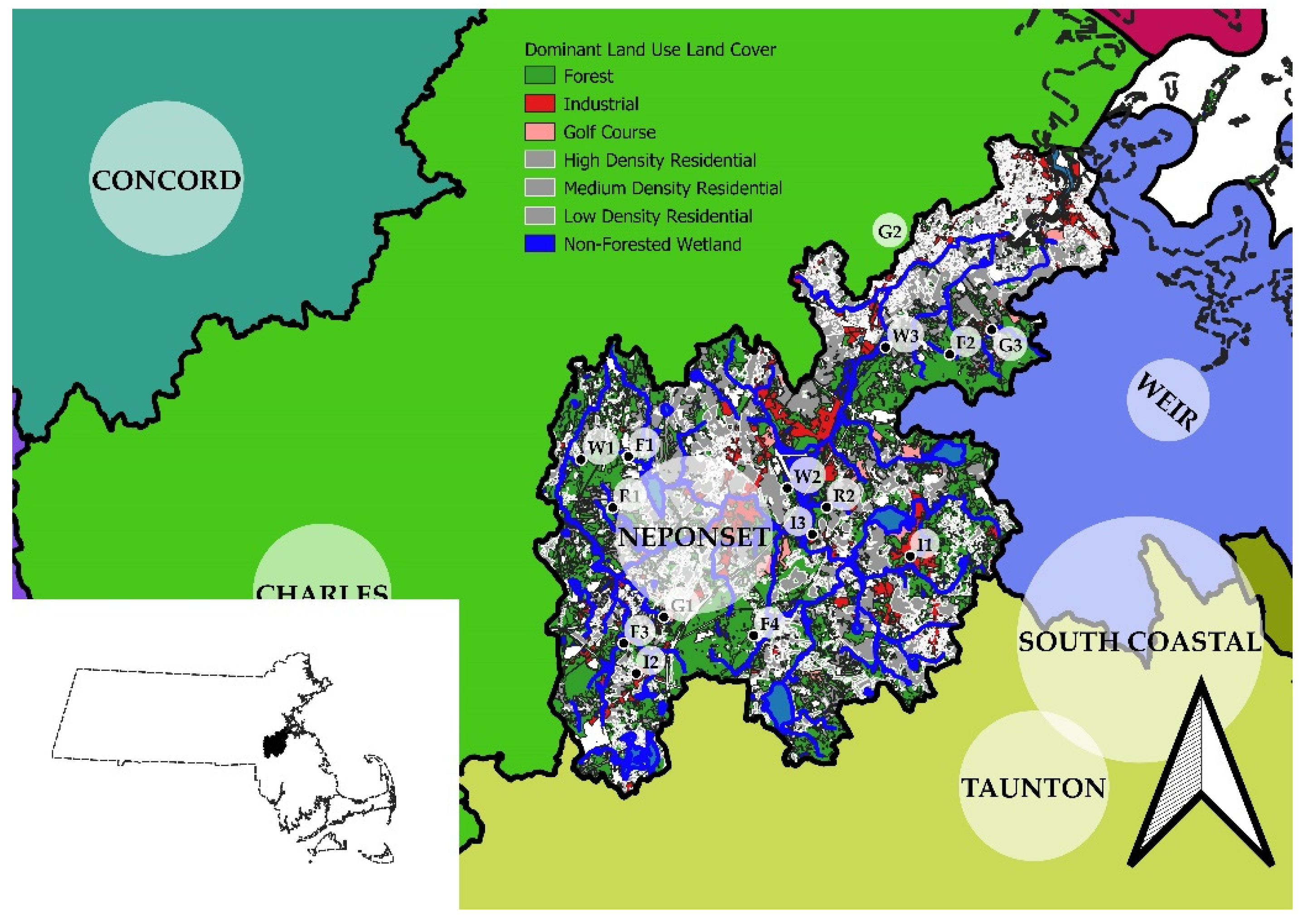
2.1. Study Area and Sampling Reaches

The Neponset River Watershed (Figure 1) is a 337 km2 urban coastal watershed located in eastern Massachusetts, U.S.A. The headwaters of the Neponset River begin near Foxboro, Massachusetts and travels approximately 44 km northeast before emptying into Boston Harbor near Dorchester, Massachusetts. Based on GIS analysis conducted by Huang and Chen [31], the top 5 LULCs in the watershed were residential, forested, industry, wetlands, and golf courses, representing 38%, 34%, 5%, 4%, and 2% of the watershed, respectively (Figure 1). The other land-use types found covered less than 2% of the land use in the watershed. Four of the five LULC types, except the wetlands, were designated as sampling treatments in this study. Within the watershed, 14 end-member stations, where water draining in that particular area is at least 80% of one of the above land-use types, were chosen using the GIS based study of Huang and Chen [31].
We selected eight sampling stations, representing a subset of the 14 end-member stations identified by Huang and Chen [31], based on sampling accessibility issues. These eight stations were chosen based on landowner approval access and were distributed evenly across the four LULC sampling treatments of (1) residential, (2) forested, (3) industrial, and (4) golf courses.

2.2. Physical Habitat Analyses: USEPA Rapid Bioassessment and Basin Area Stream Survey

We used the USEPA rapid bioassessment to assess the habitat at our eight LULC treatment stations in the summer of 2010 and 2012 [25]. At each station, we assessed a 100-m reach along the stream. The USEPA habitat assessment uses 10 metrics to assess the physical habitat each valuing 20 points. The 10 metrics/parameters assessed are (1) epifaunal substrate/available cover, (2) embeddedness/pool substrate characterization, (3) velocity/depth combinations/pool variability, (4) sediment deposition, (5) channel flow status, (6) channel alteration, (7) frequency of riffles/channel sinuosity, (8) bank stability, (9) bank vegetative protection, and riparian vegetative zone width. Total quantitative scores between 200 and 160 indicate “optimal” habitat quality, scores between 159 and 110 indicate “sub-optimal” habitat quality, scores between 109 and 60 indicate “marginal” habitat conditions, and scores less than 60 indicate “poor” habitat quality.
We conducted a Basin Area Stream Survey (BASS) [32,33] to characterize geomorphology, substrate, instream cover, and riparian cover across the 100-m station reaches in August of 2012. Within each 100-m reach, macro-habitats were identified (e.g., riffle, run, pool, backwater, etc.), and each macro-habitat was divided into transects that represented the quarter, midpoint, and three-quarter marks between the left and right banks. At each transect, the bankfull width, water width, thalweg, and depth at each quarter mark were measured using a measuring tape and a meter stick. Bank angles at the left and right banks were measured using a clinometer. The bottom substrate cover, instream cover, and riparian cover was estimated at each macro-habitat. These metrics were quantified by taking an estimation of the percent coverage at each macro-habitat. This resulted in 33 habitat variables for reach station macro-habitat site (Appendix A1).

2.3. FWI Assemblage Assessment

We collected FWI using the USEPA 20 jab dip-net method in the summer 2010 and 2012 in the same 100-m habitat reaches [25]. The FWI dip-net samples were preserved in 10% formalin and stored in the laboratory until processing. The FWI samples were processed by picking FWI using forceps and sorting the FWI into morphological groups. Morphological groups were stored in 70% ethanol. The FWI morphological groups were identified to the family taxonomic level using dichotomous keys [34,35,36,37,38].
Water-quality scores based on FWI were quantified using metric scores from the Family Biotic Index (FBI) [27] and the USEPA’s Streamside Biosurvey Index (SBI) [30]. The FBI metrics rate taxa families on the scale of 0 to 10 with 0 being the most sensitive and 10 being the most tolerant. The FBI is calculated by multiplying the total number of the families by their tolerance values. The results of all these multiplications are then summed and divided by the total number of the organisms in the sample. Ideally, the FBI should be a low number, which indicates an overall sensitive community. Higher values indicate increasing numbers of tolerant organisms dominating the community. Tolerance values from 0 to 3.75 indicates “excellent” water quality; 3.76 to 4.25 indicates “very good” water quality; 4.26 to 5 indicates “good” water quality; 5.01 to 5.75 indicates “fair” water quality; 5.76 to 6.50 indicates “fairly poor” water quality; 6.51 to 7.25 indicates “poor” water quality; and 7.26 to 10 indicates “very poor” water quality [27]. Meanwhile, the USEPA Streamside Biosurvey Index (SBI) protocol groups FWIs into three categories based on their pollution tolerance or sensitivity [30]. The categories are sensitive, somewhat sensitive, and tolerant. The water quality index is calculated by counting the taxa in each of the sensitivity categories and determining whether they are rare (R) (1 to 9 organisms), common (C) (10 to 99 organisms), or dominant (D) (100 or more organisms). The number of taxa in each category is multiplied by a weighting factor. All scores are added together and compared to a water quality rating scale. The criteria for the ratings are as follows: less than 19.9 indicates “poor” water quality; 19.9 to 39.6 indicates “fair” water quality; 39.7 to 59.4 indicates “good” water quality; and 59.5 to 79 indicates “excellent” water quality [30].

2.4. Statistical Analysis

The FWI richness, evenness, Shannon’s diversity index, and Simpson’s diversity index were calculated for each sampling station event using PC-Ord Software (Version 6) [39]. PC-Ord was also used to conduct a principal component analysis (PCA) for exploratory data analysis and data reduction in the 32 macro-habitats variables of the BASS assessment and for a non-metric multidimensional scaling analysis using FWI composition for exploratory data analysis and data reduction in the FWI assemblages at the land-use land-cover sampling treatment stations in the Neponset River Watershed. We also conducted a correlation and regression analysis of the habitat quality index versus FWI, FBI, and SBI indices, in which we expected a positive correlation between habitat quality scores and SBI scores and a negative correlation between habitat quality scores and FBI scores.

3. Results

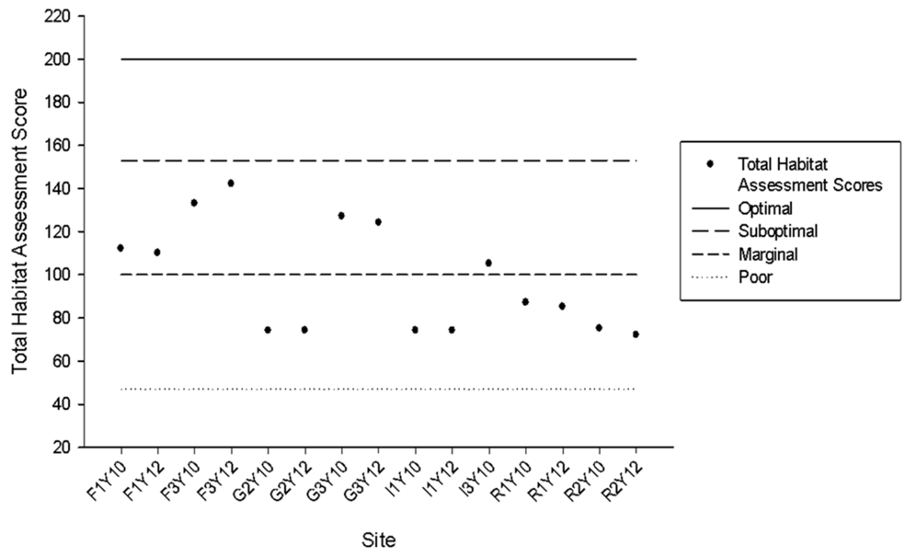
3.1. Habitat Assessment

Overall, the USEPA habitat rapid bioassessment scores ranged from a low of 72 (i.e., “marginal” habitat quality) to a high of 142 (i.e., “suboptimal” habitat quality) for both the 2010 and 2012 sampling events (Figure 2). Furthermore, the habitat assessment scores showed little change from 2010 to 2012 for most stations (Figure 2). In terms of assessment narratives, no stations were found in the “optimal” and “poor” assessment levels, however, Forest 1, Forest 3, and Golf 3 had “suboptimal” habitat quality in both years. Meanwhile, Golf 2, Industrial 1, Residential 1, and Residential 2 had “marginal” habitat quality for both years.

3.2. Habitat Characterization

While comparisons of Eigenvalue scores and Broken-stick Eigenvalue scores indicated 9 informative axes for our BASS habitat characterization PCA, we focused our interpretations of the first 2 axes, which represented ~32% of the variation in the dataset (Table 1). Overall, the first two axes showed some separation of macro-habitats of the land use/land cover sampling treatment stations (Figure 3). Based on Kendall’s tau values of > ±0.210, stations with negative scores along Axis 1 positively correlated with the habitat variables of length, bankfull width, water width, depth at the quarter transect, cobble bottom substrate, small woody debris, terrestrial vegetation, clinging vegetation, and bank stability. Stations with positive scores along Axis 1 were positively correlated with canopy coverage, sand bottom substrate, and undercut banks. Stations with negative scores along Axis 2 were positively correlated with thalweg measurements, depths at each quarter transect with the macro-habitat, terrestrial vegetation, and sand and fine bottom substrate. Stations with positive scores along Axis 2 were positively correlated with bank stability, cobble bottom substrate, and instream cover characteristics including embeddedness, clinging vegetation, and the presence of boulders. No informative clustering pattern was discerned for the sampling year, LULC sampling treatment, or macro-habitat type.

3.3. FWI Assemblage Diversity

Richness ranged from 6 (Forest 1 and 3) to 19 at Residential 2 in 2010, while in 2012 richness ranged from 3 at Golf 2 to 11 at Forest 3 and Industrial 1 (Table 2). In 2010, Evenness ranged from 0.402 at Forest 3 to 0.945 at Golf 2, while in 2012 Evenness ranged from 0.252 at Golf 2 to 0.046 at Forest 1 (Table 2). Shannon’s Diversity in 2010 ranged from 0.720 at Forest 3 to 2.126 at Industrial 3, while in 2021 Shannon’s Diversity ranged from 0.490 at Golf 2 to 2.051 at Forest 3. Simpsons Diversity ranged from 0.3176 at Forrest 3 to 0.8639 at Golf 2 in 2010 and from 0.1925 at Golf 2 to 0.8371 at Forest 3 in 2012 (Table 2).

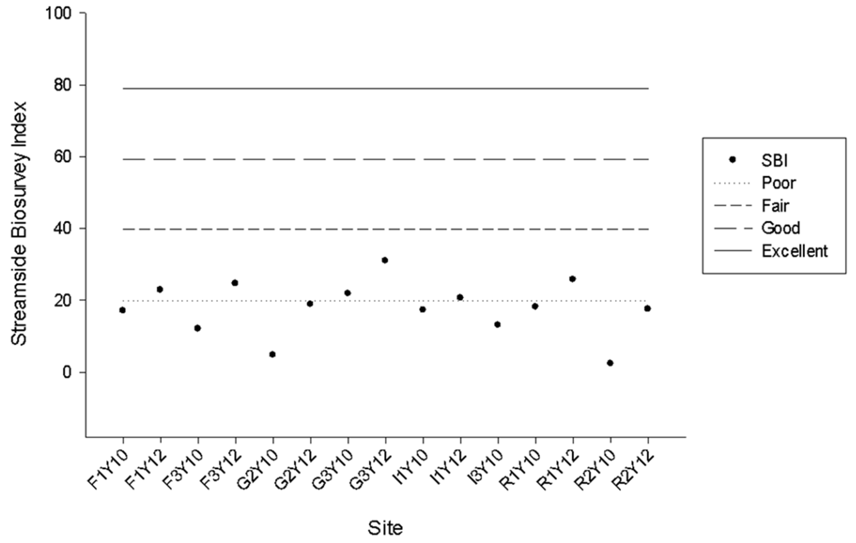
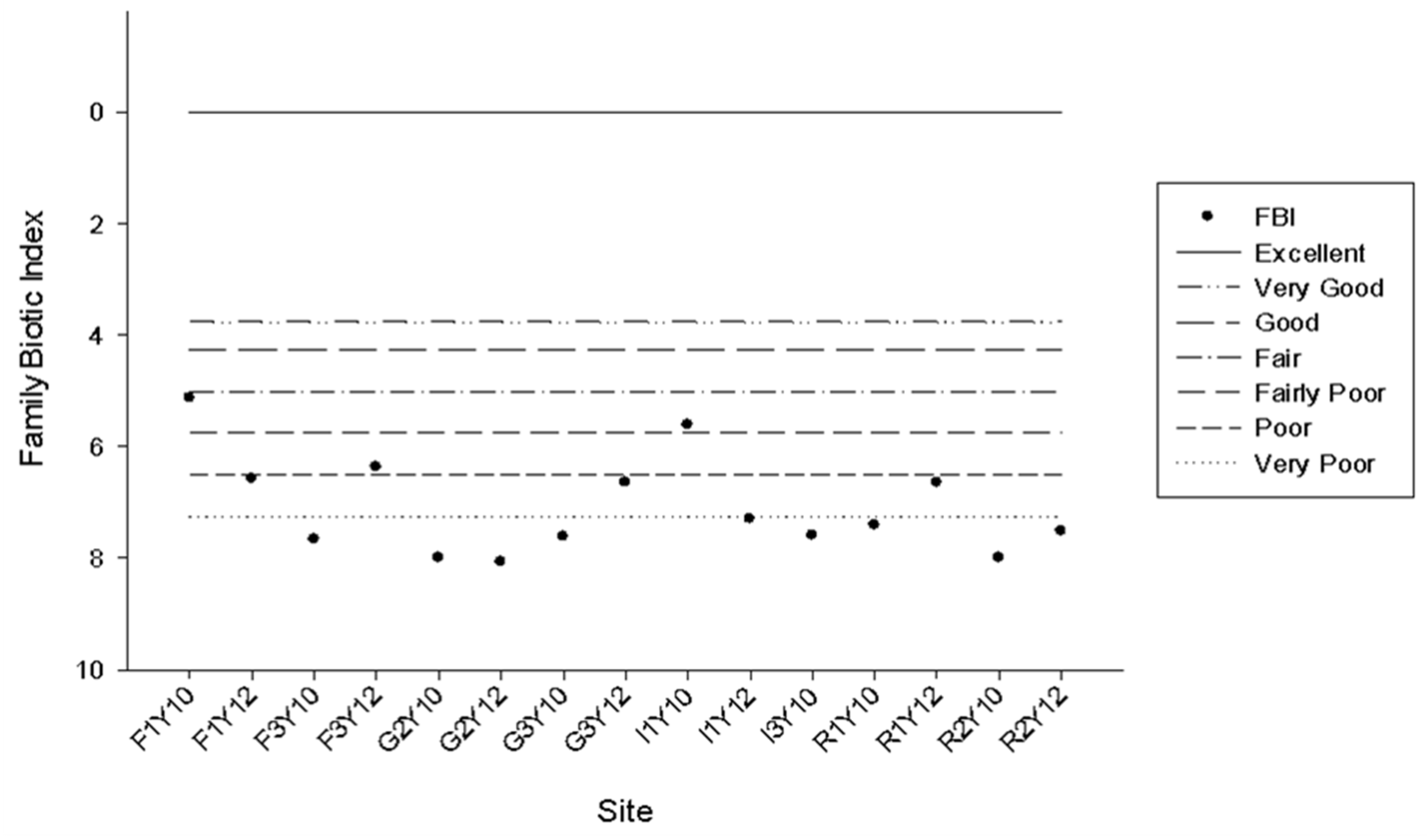
3.4. FWI Water Quality Assessment

The USEPA SBI for the Neponset River watershed indicated water quality assessments ranging from “poor” to “fair” (Figure 4). Assessment scores were generally higher in 2012 in comparison to 2010. In 2010, SBI scores ranged from a low of 2.3 (poor) at Residential 2 to a high of 21.8 (fair) at Golf 3, while in 2012 SBI scores ranged from a low of 17.5 (poor) at Residential 2 to a high of 30.9 (fair) at Golf 3 (Figure 4; Table 3).
Meanwhile, the Hilsenhoff FBI resulted in “very poor” to “good” water quality at land use cover sampling stations (Figure 5). In 2010, Hilsenhoff FBI scores ranged from a low of 5.13 (good) at Forest 1 to a high of 8.0 (very poor) at Golf 2 and Residential 2 (Figure 5; Table 3). Meanwhile, in 2012, Hilsenhoff FBI scores ranged from a low of 6.37 (fairly poor) at Forest 3 to a high of 8.06 (very poor) at Golf 2 (Figure 5; Table 3).

3.5. Habitat Quality versus FWI Water Quality Scores

Contrary to our expectation of significant correlations between USEPA habitat quality scores and FBI (negative correlation) and SBI (positive correlation) water quality scores, we did not find any statistically significant correlations, even though the data trends matched the expected correlation. We observed a non-significant negative correlation between habitat quality and FBI (Regression, df = 1, 13, r = −0.348, p = 0.207; Table 3). Furthermore, we observed a non-significant positive correlation between habitat quality and SBI (Regression, df = 1, 13, r = 0.400, p = 0.140; Table 3).

3.6. FWI Assemblage Structure Analysis

A non-metric multidimensional scaling analysis of 2010 and 2012 FWI explained ~87% of the variation in the dataset. The final stress value for this three-dimensional solution was ~5, indicating a good ordination with no real risk of drawing false inferences [39,40] (Table 4). Axis 1 and 2 explained ~58% of the variation, axis 1 and 3 ~45% of the variation, and Axis 2 and 3 explained ~71% of the variation (Figure 6, Figure 7 and Figure 8). To help interpret the non-metric multidimensional scaling results, we identified FWI associated with the axes 1–3 and their tolerance to poor water-quality conditions (Table 5).

3.6.1. Axis 1 and 2

Axes 1 and 2 were informative in separating FWI reach sampling events (Figure 6). Axis 1 was negatively correlated with two taxa (Nematoda and Oligochaeta) and positively correlated with 16 taxa (Asellidate, Caenidae, Coenagrionidae, Chironomidae, Dyticidae, Elimidate, Gammaridae, Comphidae, Halicidae, Libellulidae, Ptychopteridae, Sialidae, Spheridae, Tabariidae, Talitridae, and Turbellaria). Axis 2 was negatively correlated with 12 taxa (Calopterygidae, Chirinomidae, Elmidae, Gerridae, Halicidae, Hirudinea, Hydropsychidae, Oligochaeta, Physidae, Sphaeridae, and Tipulidae) and positively correlated with 2 taxa (Hyalellidae and Psychopteridae).
Stations with positive correlations along Axis 1 and negative correlations along Axis 2 included Golf 3 and Industrial 1 in 2012 (Figure 6). The FWI that dominated these stations included species from 24 families (Table 5). Families with high pollution tolerances levels included Asellidae, Caenidae, Coenagionidae, Halictidae, Libellulidae, Tabanidae, Ptychopteridae, Sphariidae, Talitridae, Hirudinea, Oligochaeta, and Physidae. Families with moderate pollution tolerances included Sialidae, Planorbidae, and the Turbellaria class while families with low pollution tolerances include Chirinomidae, Dytiscidae, Elimidae, Gammaridae, Gomphidae, Calopterygidae, Gerridae, Hydropsychidae, and Tipulidae.
Conversely, stations with negative correlations along Axis 1 and positive correlations along Axis 2 included Golf 3, Industrial 1, Forest 3, and Residential 2 from the 2010 sampling event (Figure 6). These stations were dominated by FWI taxa from 4 families (Table 5). Families with high pollution-tolerance levels included Hyalellidae and Oligochaeta and families with low pollution-tolerance levels included Psychomyiidae and Nematoda.
Stations with negative correlations along axes 1 and 2 included Residential 1 and Golf 2 in 2010 and 2012, Residential 2 in 2012, and Industrial 3 from 2010. These stations were dominated by FWI species from 14 families. Families with high pollution tolerances included Oligochaeta, Halictidae, Hirundinae, and Physidae, families with moderate pollution tolerances included Planorbidae and Sphaeriidae, and families with low pollution tolerances included Calopterygidae, Chironomidae, Elmidae, Gerridae, and Tipulidae.
Stations with positive correlations along axes 1 and 2 included Forest 1 in 2010 and 2012 and Forest 3 in 2012 (Figure 6). These stations were dominated by FWI assemblages from 18 families (Table 5). Those families with high pollution tolerances included Asellidae, Caenidae, Coenagionidae, Halictidae, Hyalellidae, Libellulidae, Tabanidae, Ptychopteridae, and Talitridae. Those families with moderate pollution tolerances included Sphariidae, Sialidae and the class Turbellaria. Families with low pollution tolerances included Chirinomidae, Dytiscidae, Elmidae, Gammaridae, Gomphidae, and Psychomyiidae.

3.6.2. Axis 1 and 3

Axis 1 versus 3 were informative in separating FWI reach sampling events (Figure 7). Axis 1 was negatively correlated with two taxa (Nematoda and Oligochaeta) and positively correlated with 16 taxa (Asellidate, Caenidae, Coenagrionidae, Chironomidae, Dyticidae, Elimidate, Gammaridae, Comphidae, Halicidae, Libellulidae, Ptychopteridae, Sialidae, Spheridae, Tabariidae, Talitridae, and Turbellaria). Axis 3 was negatively correlated with 2 taxa (Ceratopogonidae and Hydropsychidae) and positively correlated with 7 taxa (Chironomidae, Dyticidae, Gelastocoridae, Hyalellidae, Odontoceridae, Polycentropodidae, and Psephenidae).
Stations with positive correlations along Axis 1 and negative correlations along Axis 3 included Forest 1 form 2010 and Industrial 1 from 2012 (Figure 7). These stations were dominated by FWI assemblages from 18 families (Table 5). Those families with high pollution tolerances included Asellidae, Caenidae, Coenagionidae, Halictidae, Libellulidae, Tabanidae, Ptychopteridae, and Talitridae. Those families with moderate pollution tolerances included Sphariidae, Sialidae, Ceratopogonidae, and the class Turbellaria. Families with low pollution tolerances included Chirinomidae, Dytiscidae, Elmidae, Gammaridae, Gomphidae, and Hydropsychidae.
Those stations with negative correlations along Axis 1 and positive correlations along Axis 3 included Industrial 1 from 2010, Industrial 3 from 2010, Residential 1 and Residential 2 from 2010 and 2012, and Golf 2 from 2010 (Figure 7). These stations were dominated by FWI from 9 families (Table 5). Those families with high pollution tolerances included Oligochaeta and Hyalellidae. The family with a moderate tolerance level included Odontoceridae. Those families with low pollution-tolerance levels included Nematoda, Chirinomidae, Dytiscidae, Polycentropodidae, and Psephenidae. The Gelastocoridae family tolerance level is undetermined.
Those stations with negative correlations along axes 1 and 3 included Forest 3 and Golf 3 from 2010 and Golf 2 from 2012. These stations were dominated by FWI assemblages from 4 families. The families with a high pollution tolerance included Oligochaeta. The families with a moderate tolerance included Ceratopogonidae. Those families with low pollution tolerances included Nematoda and Hydropsychidae.
Those stations with positive correlations along axes 1 and 3 included Forest 1 and Forest 3 from 2012 and Golf 3 from 2012. These stations were dominated by FWI assemblages from 21 families. The families with high pollution tolerances included Asellidae, Caenidae, Coenagionidae, Halictidae, Hyalellidae, Libellulidae, Tabanidae, Ptychopteridae, and Talitridae. The families with moderate pollution tolerances included Sphariidae, Sialidae, Odontoceridae, and the class Turbellaria. Families with low pollution tolerances included Chirinomidae, Dytiscidae, Elmidae, Gammaridae, Gomphidae, Polycentropodidae, and Psephenida. The Gelastocoridae family tolerance level is undetermined.

3.6.3. Axis 2 and 3

Axis 2 versus 3 were informative in separating FWI reach sampling events (Figure 8). Axis 2 was negatively correlated with 12 taxa (Calopterygidae, Chirinomidae, Elmidae, Gerridae, Halicidae, Hirudinea, Hydropsychidae, Oligochaeta, Physidae, Sphaeridae, and Tipulidae) and positively correlated with 2 taxa (Hyalellidae and Psychopteridae). Axis 3 was negatively correlated with 2 taxa (Ceratopogonidae and Hydropsychidae) and positively correlated with 7 taxa (Chironomidae, Dyticidae, Gelastocoridae, Hyalellidae, Odontoceridae, Polycentropodidae, and Psephenidae).
The stations with positive correlations along Axis 2 and negative correlations along Axis 3 included Forest 1, Forest 3, and Golf 3 from 2010 and Industrial 1 from 2012 (Figure 8). These stations were dominated by FWI assemblages from 4 families. The family with a high pollution-tolerance level included Hyalellidae. The family with a moderate pollution-tolerance level included Certopogonidae. The families with a low pollution-tolerance level included Hydropsychidae and Psychomyiidae.
The stations with negative correlations along Axis 2 and positive correlations along Axis 3 included Residential 1 from 2010 and 2012, Golf 2 and Industrial 3 from 2010, and Golf 3 from 2012. These stations were dominated by FWI assemblages from 18 families. The families with high pollution-tolerance levels included Halictidae, Hirundinea, Physidae, Oligochaeta, and Hyalellidae. The families with moderate pollution-tolerance levels included Planorbidae, Sphaeriidae, and Odontoceridae. The families with low pollution-tolerance levels included Calopterygidae, Chirinomidae, Elmidae, Gerridae, Hydropsychidae, Tipulidae, Dytiscidae, Polycentropodidae, and Psephenidae.
The only station with negative correlations along both axes 2 and 3 was Golf 2 in 2012. This station was dominated by FWI from 13 families. The families with high pollution-tolerance levels included Halictidae, Hirudinea, Oligochaeta, and Physidae. Those families with moderate pollution-tolerance levels included Ceratopogonidae, Planorbidae, and Sphaeriidae. The families with low tolerance levels included Calopterygidae, Chirinomidae, Elmidae, Gerridae, Hydropsychidae, and Tipulidae.
The stations with positive correlations along both axes 2 and 3 included Forest 1 and Forest 3 from 2012, Residential 3 from 2010, and Industrial 1 from 2010. These stations were dominated by FWI assemblages from 8 families. The family with a high pollution-tolerance level included Hyalellidae. The family with a moderate pollution-tolerance level included Odontoceridae. The families with low pollution-tolerance levels included Psychomyiidae, Chirinomidae, Dytiscidae, Polycentropodidae, and Psephenidae. The Gelastocoridae family tolerance level is undetermined.

4. Discussion

We identified five major findings from our study. Our first finding was that habitat quality in the Neponset River watershed was somewhat degraded relative to pristine conditions. Our second finding was that our habitat characterization analysis observed some separation of our reach scale macrohabitat types at LULC stations with some correlations with microhabitat variables. Our third finding was that the water quality based on FWI assemblages was generally degraded in relative to pristine conditions. Our fourth finding was that contrary to our expectations, there was no significant correlation between our reach-scale USEPA habitat quality scores and FWI water-quality scores. Our fifth finding was that our FWI assemblage NMS showed separation of LULC sampling stations and that that low pollution-tolerant taxa dominated some of our LULC sampling treatment stations and influenced NMS groupings.

4.1. Habitat Quality

Our habitat-quality analyses resulted in marginal to suboptimal habitat quality that was not necessarily related to LULC sampling treatment groups, which is consistent with previous reports [41,42,43]. Our habitat-quality results suggest that local reach-scale habitat, not specifically the LULC type, has the most influence on FWI assemblages in the Neponset River watershed. Other studies have suggested that the physical habitat at the local scale in a particular LULC station may best predict the ecological response at that station [41,42,43]. In urban systems, it can be difficult to find linear relationships between stream system characteristics and LULC [44]. In pristine systems, much like the one modeled in the River Continuum Concept, one would expect that forested land-use types would be different than the more human impacted land uses. Though we found that our forested sites had the best habitat quality, as shown using the USEPA rapid bioassessment, our Golf 3 site also had higher “suboptimal” habitat quality compared to other LULC treatment stations.

4.2. Habitat Characterization

For our BASS characterization, we expected to see separation and clustering amongst similar LULC sampling treatment sites in our PCA analysis; however, our results illustrated some clustering of micro-habitats within treatment LULC stations. Forest 1 and Golf 3 were two stations in which the macro-habitats clustered together. The similar habitat characteristics that these sites exhibited included cobble bottom substrate, instream cover, and the presence of terrestrial vegetation. Theodoropoulos and Iliopoulou-Georgudaki [45] found similar habitat characteristics with low amounts of fine sediment and thicker riparian zones. These habitats are extremely favorable to FWI assemblages that have low pollution tolerance [45]. The Residential station and the Golf 2 site were dominated by a fine and sandy bottom substrate, which is not a favorable habitat for FWI species that are impacted by high pollution [45,46].

4.3. FWI Water Quality Assessment

In our study, FBI and SBI illustrated water quality in the Neponset River watershed ranging from “fair” to “very poor” and “fair” to “poor”, respectively. Our Neponset results were slightly lower than other similar watershed-scale studies. For example, Heidkamp and Christian [47] found “fair” to “good” water quality, based on SBI assessment, in a nearby urban coastal watershed, while Klauda et al. [48] used a modified Hilsenhoff biotic index across six basins/watersheds in Maryland and reported 36% were “good”, 55% were “fair”, and 9% were “poor”in terms of water quality. In trying to contextualize our results based on the major LULC in the Neponset River watershed in which we framed our sampling design, overall, our results are a bit surprising. For example, other studies have shown that forested LULC typically results in higher biological integrity scores [16,49] with relative degradation in biological integrity with increasing agriculture and urbanization. Thus, our overall water quality/biological integrity results are likely due to three out of four of our LULC sampling treatments (based on dominant coverage in the watershed) are along an “urban” LULC gradient.
When assessing water quality using biological metrics, every metric or index is different; thus, one index may be more applicable to the aquatic system of interest than another metric [50]. In our study, the SBI showed slight increases in water quality from 2010 to 2012, whereas the FBI did not show the same trend. In fact, the FBI showed that some sites declined in water quality from 2010 to 2012. Different water quality assessments also can produce varying conclusions about the water pollution levels in that system. The SBI indicated that our sites in the Neponset River watershed had water quality ranging from “poor” to “fair”, while the FBI indicated water quality ranging from “very poor” to “fairly poor”. The FBI also has seven pollution levels whilst the SBI only has four, which creates issues in relative scales. In systems such as agricultural systems, FBI may be more useful because of its focus on family tolerance [27,51]. When applying or adjusting best management practices in agricultural systems, the FBI can better show the response of the FWI community. For instance, going from “poor” to “fairly poor” is very achievable by making a small change in riparian zone coverage or increasing buffer zone areas. Conversely, the SBI is a more useful tool in the urban system where there are many different LULC types. The SBI is based on the richness and abundance of different tolerance groups, which is very effective for characterizing stream water quality and determining trends over yearly periods [30].

4.4. Habitat Quality versus FWI Water Quality

Based on theoretical and empirical reports [9,10,52,53], we expected a statistically significant correlation between our USEPA physical habitat index scores and our rapid bioassessment SBI (positive correlation) and FBI (negative correlation). While these correlations were observed as expected, they were not statistically significant. Similar findings were found when relating urban and non-urban land uses with collector and gatherer FWI assemblages in southeastern Wisconsin streams [54]. Our insignificant findings could be due to the local-scale analysis of habitat quality and that factors at larger scales may have direct and indirect effects on the stream habitat and water quality at larger spatial scales. For example, larger catchment scale studies have better shown correlations between impervious land uses and degradation of macroinvertebrate assemblages independent of habitat-quality scores [54,55,56,57].

4.5. FWI Assemblage Analysis

Multivariate analysis of FWI assemblages, not including rapid bioassessment indices of biotic integrity, have been used as surrogate indicators of water quality across the globe [21,22,23,24,45,58]. Brito et al. [24] reported that taxonomic and functional metrices responded similarly to a variety of environmental conditions and were reasonable biological indicators for assessing and conserving streams influenced by agriculture in Amazon streams. Theodoropoulos and Iliopoulou-Georgudaki [45] found that FWI assemblage diversity was strongly correlated to pollution at sites with major environmental stressors, and physical habitat degradation showed low species richness and diversity while sites less impacted were characterized by higher diversity. In Kenyan streams, macroinvertebrate assemblages were shown to respond to changes in land use and water quality in which key macroinvertebrates taxa were identified to monitor changes in water quality [21].
Though dominated by highly pollution-tolerant FWI families, our non-metric multidimensional scaling multivariate FWI assemblage analysis identified that Golf 3 from the 2012 sampling event season was controlled by 24 families. Out of those 24 families, 12 were moderate to low pollution-tolerant species and the other 12 were high pollutant-tolerant species. Likewise, the Forest 1 site in 2010 was dominated by FWI species from 18 families. Out of those 18 families, 10 were moderate-to-low pollution tolerant, and the other were from highly pollution-tolerant families. Golf 3 and Forest 1 were the two sites where the habitat was most favorable for FWI species, and here, we find that though there are organisms from highly tolerant families, these two sites had the highest diversity.

5. Conclusions

In terms of our hypotheses, we expected that the habitat quality of LULC much different than its natural state or with high human influence would be different from the LULC stations closest to a natural state. We found that our forested sites exhibited an overall better habitat quality compared to our other LULC treatment sites. One of our golf sites unexpectedly had a higher habitat quality than forested sites. We also hypothesized that FWI assemblages would ultimately be a reflection of the habitat quality. We found that habitat quality showed little impact on the FWI assemblages as some LULC treatments with better habitat quality had FWI assemblages indicative of poorer water quality. Other local-scale influences, or possibly one habitat metric more than the other, may be of greater impact to the FWI assemblages. Lastly, we further hypothesized that FWI assemblages will vary based on the LULC treatments and that specific FWI would be associated with the LULC type because of the quality of the water at that site. However, we found that all LULC sampling treatment stations were dominated by highly pollution-tolerant organisms.
Global change drivers such as habitat degradation, climate change, invasive species, overexploitation, and pollution will continue to impact stream ecosystems [59]. Therefore, baseline studies such as our catchment and reach-scale habitat and FWI assemblage case-study are important efforts to establish baseline conditions for future monitoring efforts and current management planning. For example, we concluded that biotic integrity-based water quality is degraded in the watershed and that reach-scale habitat alone did not solely influence the FWI assemblages in the Neponset River watershed. Other factors such as catchment-scale LULC or other drivers are likely contributors to the variability in our FWI assemblage composition, diversity, and integrity scores. There are a variety of restoration actions that can be implemented to improve water quality and ecosystem services in the Neponset River watershed. However, a recent sustainable stream restoration review suggests that managers and stakeholders use a bottom-up framework (socioeconomic, hydrologic, hydraulic, geomorphic, physiochemical, biological) in their restoration efforts, in which starting with socioeconomic factors and processes will likely lead to better outcomes on individual projects and sustainable support for future restoration efforts [60].

Author Contributions

Conceptualization, A.D.C. and N.D.H.; methodology, A.D.C. and N.D.H.; software, A.D.C.; validation, A.D.C. and N.D.H.; formal analysis, A.D.C. and N.D.H.; investigation, N.D.H.; resources, N.D.H.; data curation, N.D.H.; writing—original draft preparation, N.D.H.; writing—review and editing, A.D.C. and N.D.H.; visualization, A.D.C. and N.D.H.; supervision, A.D.C.; project administration, A.D.C.; funding acquisition, A.D.C. All authors have read and agreed to the published version of the manuscript.

Funding

This research was partially supported by the Biology Department at the University of Massachusetts Boston as start-up funds to A.D.C. and National Science Foundation Research Experiences for Undergraduates funding to A.D.C. via NSF-OCE-1062374 (Hannigan and Christian) and NSF-OCE-1359242 (Christian and Hannigan).

Institutional Review Board Statement

Not applicable.

Informed Consent Statement

Not applicable.

Data Availability Statement

Data for this project are held by both ADC (copies) and NH (original) in laboratory handbooks and excel data sheets on personal computer hard drives. Request for data may be directed to the corresponding author.

Acknowledgments

Field and laboratory assistance were provided by Deirdre Burk, Kelly Canesi, Thomas Dimino, Llewin Froome, Melanie Garate, David Kemp, Sean McCanty, Allie Ruan, Rosemary Schuster, Michael Simmons, and Alexander Webley. Early drafts of this manuscript were improved through N.D.H dissertation committee members Solange Brault, Robert Chen, Robyn Hannigan, and Michael Shiaris.

Conflicts of Interest

The authors declare no conflict of interest. The funders had no role in the design of the study; in the collection, analyses, or interpretation of data; in the writing of the manuscript, or in the decision to publish the results.

Appendix A

Table A1. Acronym term definitions for the 33 Basin Area Stream Survey variables.
AcronymTermAcronymTerm
LGRLow gradient riffleICEMBInstream-cover Embeddedness
HGRHigh gradient riffleICUCBInstream-cover undercut banks
BWPBack-water poolICLWDInstream-cover large woody debris
PLPPlunge poolICSWDInstream-cover small woody debris
LGPLog lateral scour poolICWWInstream-cover whitewater
DLPDammed poolICBOInstream-cover boulder
RUNRunICBRLInstream-cover bedrock ledge
CCPChannel confluence poolICCLNInstream-cover clinging vegetation
CRPCorner poolICRTInstream-cover rooted vegetation
LSPLateral scour poolLFTBKLeft bank angle
LENMacrohabitat lengthLFTSLeft bank stability
BFWBankfull widthLFTVVLeft bank terrestrial vegetation
WAWIDWater widthMIDCMid-channel canopy
THALThalweg depthRGTBKRight bank angle
DEPLSDepth left bankRGTSRight bank stability
DEP25Depth ¼ width from left bankRGTVVRight bank terrestrial vegetation
DEP 50Depth ½ width from left bankFForest
DEP 75Depth ¾ width from left bankGGolf
DEPRSDepth right bankIIndustrial
BTBo% bottom bouldersRResidential
BTMC% bottom cobbleY102010
BTMG% bottom gravelY122012
BTMS% bottom sand
BTMF% bottom fines

References

  1. Malmqvist, B.; Rundle, S. Threats to the running water ecosystems of the world. Environ. Conserv. 2002, 29, 134–153. [Google Scholar] [CrossRef]
  2. Dudgeon, D.; Arthington, A.H.; Gessner, M.O.; Kawabata, Z.-I.; Knowler, D.J.; Lévêque, C.; Naiman, R.J.; Prieur-Richard, A.-H.; Soto, D.; Stiassny, M.L.J.; et al. Freshwater biodiversity: Importance, threats, status and conservation challenges. Biol. Rev. 2006, 81, 163–182. [Google Scholar] [CrossRef] [PubMed]
  3. Reid, A.J.; Carlson, A.K.; Creed, I.F.; Eliason, E.J.; Gell, P.A.; Johnson, P.T.J.; Kidd, K.A.; MacCormack, T.J.; Olden, J.D.; Ormerod, S.J.; et al. Emerging threats and persistent conservation challenges for freshwater biodiversity. Biol. Rev. 2019, 94, 849–873. [Google Scholar] [CrossRef] [PubMed]
  4. Merriam-Webster, Incorporated. In Habitat; Merriam-Webster, Inc.: Springfield, MA, USA, 2022; Available online: https://www.merriam-webster.com/dictionary/habitat (accessed on 14 August 2022).
  5. Southwood, T.R.E. Tactics, Strategies and Templets. Oikos 1988, 52, 3–18. [Google Scholar] [CrossRef]
  6. Southwood, T.R.E. Habitat, the Templet for Ecological Strategies? J. Anim. Ecol. 1977, 46, 337–365. [Google Scholar] [CrossRef]
  7. Frissell, C.A.; Liss, W.J.; Warren, C.E.; Hurley, M.D. A hierarchical framework for stream habitat classification: Viewing streams in a watershed context. Environ. Manag. 1986, 10, 199–214. [Google Scholar] [CrossRef]
  8. Maddock, I.; Harby, A.; Kemp, P.; Wood, P.J. Ecohydraulics: An Integrated Approach; John Wiley & Sons: Hoboken, NJ, USA, 2013. [Google Scholar]
  9. Maddock, I. The importance of physical habitat assessment for evaluating river health. Freshw. Biol. 1999, 41, 373–391. [Google Scholar] [CrossRef]
  10. Raven, P.J.; Holmes, N.T.H.; Dawson, F.H.; Fox, P.J.A.; Everard, M.; Fozzard, I.R.; Rouen, K.J. River Habitat Quality: The Physical Character of Rivers and Streams in the UK and Isle of Man; Environment Agency: Bristol, UK, 1998. [Google Scholar]
  11. Nelson, G.C. Drivers of Ecosystem Change: Summary Chapter. In Ecosystems and Human Well-being: Current State and Trends; Island Press: Washington, DC, USA, 2005; Volume 1, pp. 73–76. [Google Scholar]
  12. Sala, O.E.; Chapin, F.S.; Armesto, J.J.; Berlow, E.; Bloomfield, J.; Dirzo, R.; Huber-Sanwald, E.; Huenneke, L.F.; Jackson, R.B.; Kinzig, A.; et al. Global Biodiversity Scenarios for the Year 2100. Science 2000, 287, 1770–1774. [Google Scholar] [CrossRef]
  13. Allan, J.D. Landscapes and Riverscapes: The Influence of Land Use on Stream Ecosystems. Annu. Rev. Ecol. Evol. Syst. 2004, 35, 257–284. [Google Scholar] [CrossRef]
  14. Karr, J.R. Biological Integrity: A Long-Neglected Aspect of Water Resource Management. Ecol. Appl. 1991, 1, 66–84. [Google Scholar] [CrossRef]
  15. DeShon, J.E. Development and Application of the Invertebrate Community Index (ICI). In Biological Assessment and Criteria: Tools for Risk-Based Decision Making and Planning; Davis, W.S., Simon, T., Eds.; Lewis Publishers: Boca Raton, FL, USA, 1995; pp. 217–243. [Google Scholar]
  16. Roth, N.E.; Allan, J.D.; Erickson, D.L. Landscape Influences on Stream Biotic Integrity Assessed at Multiple Spatial Scales. Landsc. Ecol. 1996, 11, 141–156. [Google Scholar] [CrossRef]
  17. Allan, J.D.; Brenner, A.J.; Erazo, J.; Fernandez, L.; Flecker, A.S.; Karwan, D.L.; Segnini, S.; Taphorn, D.C. Land Use in Watersheds of the Venezuelan Andes: A Comparative Analysis. Conserv. Biol. 2002, 16, 527–538. [Google Scholar] [CrossRef]
  18. Maloney, K.O.; Weller, D. Anthropogenic disturbance and streams: Land use and land-use change affect stream ecosystems via multiple pathways. Freshw. Biol. 2010, 56, 611–626. [Google Scholar] [CrossRef]
  19. Walsh, C.J.; Roy, A.H.; Feminella, J.W.; Cottingham, P.D.; Groffman, P.M.; Morgan, R.P. The Urban Stream Syn-drome: Current Knowledge and the Search for a Cure. J. N. Am. Benthol. Soc. 2005, 24, 706–723. [Google Scholar] [CrossRef]
  20. Roy, A.H.; Capps, K.A.; El-Sabaawi, R.W.; Jones, K.L.; Parr, T.B.; Ramírez, A.; Smith, R.F.; Walsh, C.J.; Wenger, S.J. Urbanization and stream ecology: Diverse mechanisms of change. Freshw. Sci. 2016, 35, 272–277. [Google Scholar] [CrossRef]
  21. Kilonzo, F.; Masese, F.O.; Van Griensven, A.; Bauwens, W.; Obando, J.; Lens, P.N. Spatial–temporal variability in water quality and macro-invertebrate assemblages in the Upper Mara River basin, Kenya. Phys. Chem. Earth Parts A/B/C 2014, 67–69, 93–104. [Google Scholar] [CrossRef]
  22. Parr, L.; Mason, C. Long-term trends in water quality and their impact on macroinvertebrate assemblages in eutrophic lowland rivers. Water Res. 2003, 37, 2969–2979. [Google Scholar] [CrossRef]
  23. Sharma, K.K.; Chowdhary, S. Macroinvertebrate Assemblages as Biological Indicators of Pollution in a Central Himalayan River, Tawi (J&K). Int. J. Biodivers. Conserv. 2011, 3, 167–174. [Google Scholar]
  24. Brito, J.G.; Martins, R.T.; Oliveira, V.C.; Hamada, N.; Nessimian, J.; Hughes, R.M.; Ferraz, S.; de Paula, F.R. Biological indicators of diversity in tropical streams: Congruence in the similarity of invertebrate assemblages. Ecol. Indic. 2018, 85, 85–92. [Google Scholar] [CrossRef]
  25. Barbour, M.T.; Gerritsen, J.; Snyder, B.D.; Stribling, J.B. Rapid Bioassessment Protocols for Use in Streams and Wadeable Rivers: Periphyton, Benthic Macroinvertebrates, and Fish; EPA 841-B-99-002, 2nd ed.; U.S. Environmental Protection Agency: Office of Water: Washington, DC, USA, 1999; Volume EPA 841-B-99-002.
  26. Hilsenhoff, W.L. Using a Biotic Index to Evaluate Water Quality in Streams; Report; Wisconsin Department of Natural Resources: Madison, Wisconsin, 1982. [Google Scholar]
  27. Hilsenhoff, W.L. Rapid Field Assessment of Organic Pollution with a Family-Level Biotic Index. J. N. Am. Benthol. Soc. 1988, 7, 65–68. [Google Scholar] [CrossRef]
  28. Karr, J.R. Assessment of Biological Integrity Using Fish Communities. Fisheries 1981, 6, 21–27. [Google Scholar] [CrossRef]
  29. Rankin, E.T.; Yoder, C.O. Methods for Assessing Habitat in Flowing Waters Using the Qualitative Habitat Evaluation Index (QHEI); Report; Ecological Assessment Unit, Division of Surface Water, Ohio EPA: Columbus, OH, USA, 1999. [Google Scholar]
  30. United States Environmental Protection Agency. Volunteer Stream Monitoring: A Methods Manual; 4503F EPA 841-B-97-003; Office of Water, Environmental Protection Agency: Washington, DC, USA, 1997; p. 227.
  31. Huang, W.; Chen, R.F. Sources and transformations of chromophoric dissolved organic matter in the Neponset River Watershed. J. Geophys. Res. Earth Surf. 2009, 114. [Google Scholar] [CrossRef]
  32. McCain, M.E.; Fuller, D.; Decker, L.; Overton, K. Stream Habitat Classification and Inventory Procedures for Northern California. Fish Habitat Relatsh. Tech. Bull. 1990, 1, 1–15. [Google Scholar]
  33. Clingenpeel, J.A.; Cochran, B.G. Using Physical, Chemical, and Biological Indicators to Assess Water Quality on the Ouachita National Forest Utilizing Basin Area Stream Survey Methods. Proc. Ark. Acad. Sci. 1992, 46, 33–35. [Google Scholar]
  34. Merritt, R.W.; Cummins, K.S. An Introduction to the Aquatic Insects of North America, 3rd ed.; Kendall/Hunt Publishing Company: Dubuque, Iowa, 1996. [Google Scholar]
  35. Rogers, D.C.; Hill, M. Key to the Freshwater Malacostraca (Crustacea) of the Mid-Atlantic Region; US EPA, Office of Environmental Information: Washington, DC, USA, 2008; Above: The exotic rusty crayfish was the only crayfish species found in the main stem of Loyalsock Creek 2008. [Google Scholar]
  36. Thorp, J.H.; Covich, A.P. Ecology and Classification of North American Freshwater Invertebrates; Academic Press, Inc: San Diego, CA, USA, 1991. [Google Scholar]
  37. Merritt, R.W.; Cummins, K.W.; Berg, M.B. An Introduction to the Aquatic Insects of North America, 4th ed.; Kendall; Hunt Publishing Company: Dubuque, IA, USA, 2008. [Google Scholar]
  38. Thorp, J.H.; Covich, A.P. Ecology and Classification of North American Freshwater Invertebrates; Academic Press: Cambridge, MA, USA, 2009. [Google Scholar]
  39. McCune, B.; Mefford, M.J. PC-ORD v. 6.255 Beta; MjM Software: Gleneden Beach, OR, USA, 2011. [Google Scholar]
  40. McCune, B.; Grace, J.B.; Urban, D.L. Analysis of Ecological Communities; MjM Software Design: Gleneden Beach, OR, USA, 2002; Volume 28. [Google Scholar]
  41. Tran, C.P.; Bode, R.W.; Smith, A.J.; Kleppel, G.S. Land-use proximity as a basis for assessing stream water quality in New York State (USA). Ecol. Indic. 2010, 10, 727–733. [Google Scholar] [CrossRef]
  42. Allan, D.; Erickson, D.; Fay, J. The influence of catchment land use on stream integrity across multiple spatial scales. Freshw. Biol. 1997, 37, 149–161. [Google Scholar] [CrossRef]
  43. Strayer, D.L.; Beighley, R.E.; Thompson, L.C.; Brooks, S.; Nilsson, C.; Pinay, G.; Naiman, R.J. Effects of Land Cover on Stream Ecosystems: Roles of Empirical Models and Scaling Issues. Ecosystems 2003, 6, 407–423. [Google Scholar] [CrossRef]
  44. Gergel, S.E.; Turner, M.G.; Miller, J.R.; Melack, J.M.; Stanley, E.H. Landscape Indicators of Human Impacts to Riverine Systems. Aquat. Sci. 2002, 64, 118–128. [Google Scholar] [CrossRef]
  45. Theodoropoulos, C.; Iliopoulou-Georgudaki, J. Response of Biota to Land Use Changes and Water Quality Degra-dation in Two Medium-Sized River Basins in Southwestern Greece. Ecol. Indic. 2010, 10, 1231–1238. [Google Scholar] [CrossRef]
  46. Chakona, A.; Phiri, C.; Magadza, C.H.D.; Brendonck, L. The influence of habitat structure and flow permanence on macroinvertebrate assemblages in temporary rivers in northwestern Zimbabwe. Hydrobiologia 2008, 607, 199–209. [Google Scholar] [CrossRef]
  47. Heidkamp, L.C.; Christian, A.D. A Case Study Evaluating Water Quality and Reach-, Buffer-, and Water-shed-Scale Explanatory Variables of an Urban Coastal Watershed. Urban Sci. 2022, 6, 17. [Google Scholar] [CrossRef]
  48. Klauda, R.; Kazyak, P.; Stranko, S.; Southerland, M.; Roth, N.; Chaillou, J. Maryland Biological Stream Survey: A State Agency Program to Assess the Impact of Anthropogenic Stresses on Stream Habitat Quality and Biota. Environ. Monit. Assess. 1998, 51, 299–316. [Google Scholar] [CrossRef]
  49. Wang, L.; Lyons, J.; Kanehl, P.; Gatti, R. Influences of Watershed Land Use on Habitat Quality and Biotic Integrity in Wisconsin Streams. Fisheries 1997, 22, 6–12. [Google Scholar] [CrossRef]
  50. Varnosfaderany, M.N.; Ebrahimi, E.; Mirghaffary, N.; Safyanian, A. Biological Assessment of the Zayandeh Rud River, Iran, Using Benthic Macroinvertebrates. Limnol. Ecol. Manag. Inland Waters 2010, 40, 226–232. [Google Scholar] [CrossRef]
  51. Roy, A.H.; Rosemond, A.D.; Leigh, D.S.; Paul, M.J.; Wallace, J.B. Habitat-specific responses of stream insects to land cover disturbance: Biological consequences and monitoring implications. J. N. Am. Benthol. Soc. 2003, 22, 292–307. [Google Scholar] [CrossRef]
  52. Nicklin, L.; Balas, M.T. Correlation between Unionid Mussel Density and EPA Habitat-assessment Parameters. Northeast. Nat. 2007, 14, 225–234. [Google Scholar] [CrossRef]
  53. Hannaford, M.J.; Resh, V.H. Variability in Macroinvertebrate Rapid-Bioassessment Surveys and Habitat Assess-ments in a Northern California Stream. J. N. Am. Benthol. Soc. 1995, 14, 430–439. [Google Scholar] [CrossRef]
  54. Stepenuck, K.F.; Crunkilton, R.L.; Wang, L. Impacts of urban landuse on macroinvertebrate communities in southeastern wisconsin streams. JAWRA J. Am. Water Resour. Assoc. 2002, 38, 1041–1051. [Google Scholar] [CrossRef]
  55. May, C.; Horner, R.R.; Karr, J.R.; Mar, B.W.; Welch, E.B. Effects of Urbanization on Small Streams in the Puget Sound Ecoregion. Watershed Prot. Tech. 1999, 2, 79. [Google Scholar]
  56. Walsh, C.J.; Sharpe, A.K.; Breen, P.F.; Sonneman, J.A. Effects of urbanization on streams of the Melbourne region, Victoria, Australia. I. Benthic macroinvertebrate communities. Freshw. Biol. 2001, 46, 535–551. [Google Scholar] [CrossRef]
  57. Walsh, C.J.; Waller, K.A.; Gehling, J.; MAC Nally, R. Riverine invertebrate assemblages are degraded more by catchment urbanisation than by riparian deforestation. Freshw. Biol. 2007, 52, 574–587. [Google Scholar] [CrossRef]
  58. Uriarte, M.; Yackulic, C.B.; Lim, Y.; Arce-Nazario, J.A. Influence of land use on water quality in a tropical landscape: A multi-scale analysis. Landsc. Ecol. 2011, 26, 1151–1164. [Google Scholar] [CrossRef] [PubMed]
  59. Kernan, M.; Battarbee, R.W.; Moss, B.R. Climate Change Impacts on Freshwater Ecosystems; John Wiley & Sons: Hoboken, NJ, USA, 2011. [Google Scholar]
  60. Hawley, R.J. Making Stream Restoration More Sustainable: A Geomorphically, Ecologically, and Socioeconomi-cally Principled Approach to Bridge the Practice with the Science. BioScience 2018, 68, 517–528. [Google Scholar] [CrossRef] [PubMed]
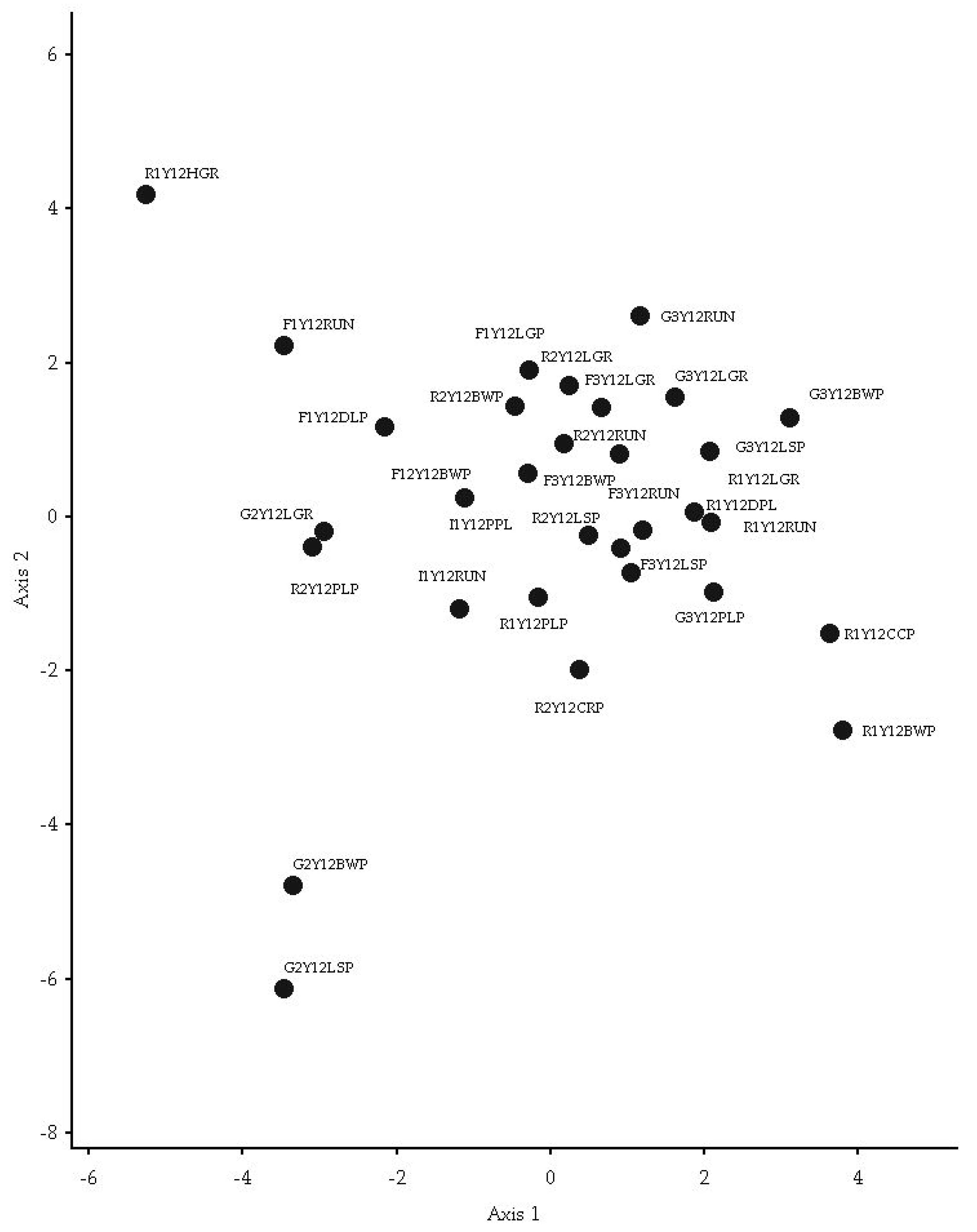
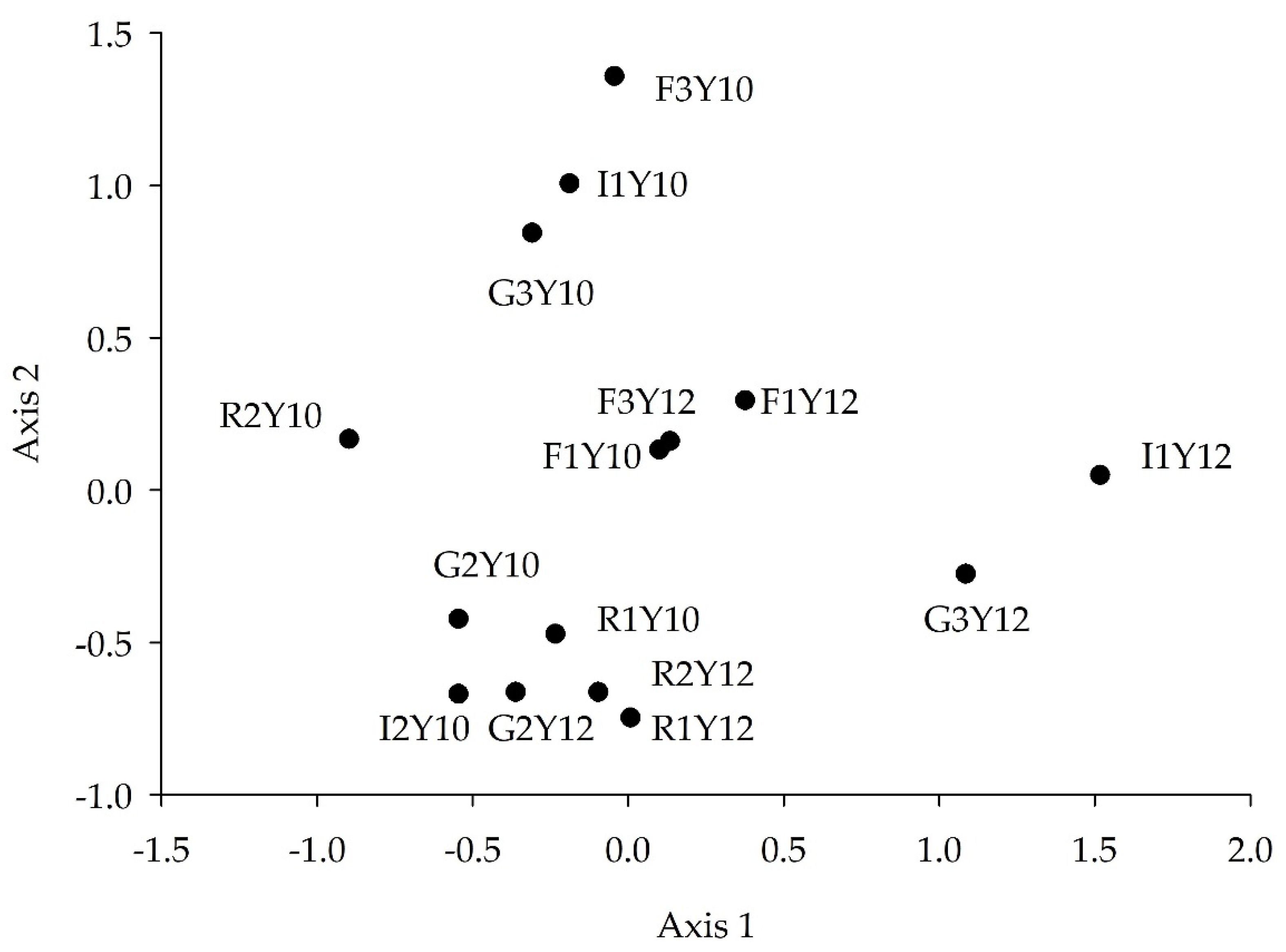
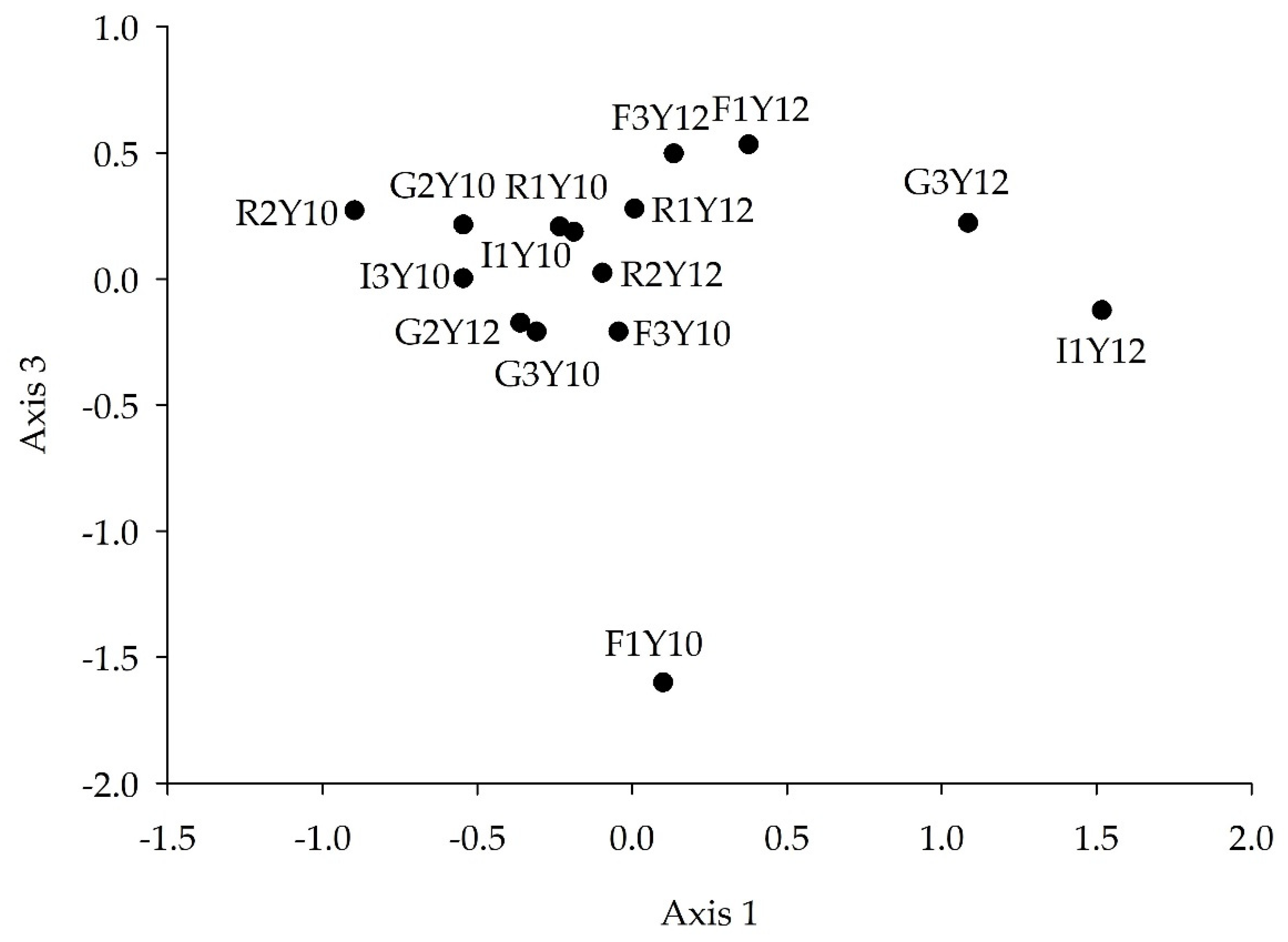
Figure 1. Map of the 14 Neponset River Watershed dominant Land Use Land Cover pore points determined by Huang and Chen31 resulting in this study’s 8 sampling stations (R = Residential; F = Forested; I = Industrial, G = Golf, W = Wetland) sampled in water year 2010 and 2012. Map created by Alan Christian.
Ecologies 03 00028 g001
Figure 2. Total habitat assessment scores from the USEPA rapid habitat bioassessment at varying Land Use Land Cover sampling treatment stations in the Neponset River watershed for August 2010 (Y10) and August 2012 (Y12). Habitat quality is ranked from “optimal” (highest) to “poor” (lowest) (F = Forested (F1 and F3); G = Golf (G2 and G3), I = Industrial (I1 and I3, and R = Residential (R1 and R3)).
Ecologies 03 00028 g002
Figure 3. Principal component analysis of the 33 Basin Area Stream Survey parameters for the 9-land use/cover stations in the Neponset River watershed (Axis 1 (17.42% of variation) vs Axis 2 (14.58% of variation)). Axis 1 is negatively correlated with LEN, BFW, WAWID, DEP25, BTMC, ICSWD, ICTV, ICCLN LFTS, LFTVV, RGTS, RGTTV and positively correlated with MIDC, BTMS, and ICUCB. Axis 2 is negatively correlated with THAL, DEP25, DEP50, DEP75, ICTV, BTMS, and BTMF and positively correlated with BTMC, ICEMB, ICBO, ICCLN, RGTBK, RGTS (F = Forested (F1 and F3); G = Golf (G2 and G3), I = Industrial (I1 and I3); R = Residential (R1 and R3); Y10 = 2010; Y12 = 2012). Basin Area Stream Survey acronym definitions are located in Table A1.
Ecologies 03 00028 g003
Figure 4. USEPA SBI scores at the 8 land use land cover treatment reaches in the Neponset River Watershed in 2010 and 2012. Higher values indicate better water quality; lower values indicate poorer water quality (F = Forest, G = Golf, I = Industrial, R = Residential; Y10 = 2010, Y12 =2012).
Ecologies 03 00028 g004
Figure 5. Family Biotic Index (FBI) scores calculated from FWI samples collected from the 8 LULC reaches in the Neponset River Watershed in 2010 and 2012. Note: for FBI, lower values indicate better water quality; higher values indicate poorer water quality (F = Forest, G = Golf, I = Industrial, R = Residential; Y10 = 2010, Y12 =2012).
Ecologies 03 00028 g005
Figure 6. Axis 1 versus 2 (58% variance explained) reach sampling event distribution of the non-metric multi-dimensional scaling analysis of FWI assemblages at 8 land use/land cover sites in 2010 and 7 sites in 2012 (F = Forest, G = Golf, I = Industrial, R = Residential; Y10 = 2010, Y12 = 2012).
Ecologies 03 00028 g006
Figure 7. Axis 1 versus 3 (45% variance explained) reach sampling event distributions for the non-metric multidimensional scaling analysis of macroinvertebrate assemblages at 8 land use/land cover sites in 2010 and 7 sites in 2012 (F = Forest, G = Golf, I = Industrial, R = Residential; Y10 = 2010, Y12 =2012).
Ecologies 03 00028 g007
Figure 8. Axis 2 versus 3 (71% variance explained) reach sampling event distributions for the non-metric multidimensional scaling analysis of macroinvertebrate assemblages at 8 land-use/land-cover sites in 2010 and 7 sites in 2012 (F = Forest, G = Golf, I = Industrial, R = Residential; Y10 = 2010, Y12 = 2012).
Ecologies 03 00028 g008
Table 1. Principal component analysis axes 1–10 summary statistics (Eigenvalue, percent of variance explained, cumulative percent of variance explained, and broken-stick eigenvalue) for Basin Area Stream Survey 2010 at 9 land-use land-cover stations in the Neponset River watershed, Massachusetts, U.S.A.
AxisEigenvalue% of VarianceCum.% of Var.Broken Stick Eigenvalue
15.05217.42117.4213.962
24.22714.57731.9982.962
32.98310.28642.2842.462
42.5578.81651.12.128
52.2637.80258.9021.878
61.8066.22665.1281.678
71.655.6970.8181.512
81.3884.78575.6031.369
91.2824.42280.0251.244
100.9583.30583.331.133
Table 2. FWI community abundance and diversity summary statistics for in the Neponset River watershed for samples collected August 2010 and August 2012 (F = Forest, G = Golf, I = Industrial, R = Residential; Y10 = 2010, Y12 =2012).
SiteMeanStd. Dev.SumRichnessEvennessShannon’s DiversitySimpson’s Diversity
F1Y20100.4221.4381960.8291.4850.7258
F1Y20120.2220.6361060.9461.6960.8000
F3Y20101.7339.5557860.4020.7200.3176
F3Y20120.8222.09237110.8552.0510.8371
G2Y20100.5781.3232690.9452.0750.8639
G2Y20123.02218.16913670.2520.4900.1925
G3Y20104.06720.584183120.4261.0580.4211
G3Y20120.63.2012730.5730.6300.3594
I1Y20106.75617.802304160.7642.1180.8269
I1Y20126.04422.983272110.6591.5810.6636
I3Y20102.5337.197114170.7502.1260.8024
R1Y20102.9569.568133130.6601.6930.7501
R1Y20124.06715.73418380.6301.3100.6525
R2Y201013.31134.651599190.7192.1160.8305
R2Y20124.420.39919870.5821.1320.5108
Table 3. Combined table data for correlations between USEPA total habitat quality scores, Streamside Biosurvey Index (SBI) scores, and Family Biotic Index (FBI) scores (Regression: Total Habitat vs. SBI r = 0.400, p = 0.140) (Total Habitat vs. FBI r = −0.348, p = 0.207) (F = Forest, G = Golf, I = Industrial, R = Residential; Y2010 = 2010, Y2012 =2012).
Sampling EventEPA HabitatSBIFBI
F1Y201011217.05.13
F1Y201211022.86.58
F3Y201013312.07.66
F3Y201214224.66.37
G2Y2010744.78.00
G2Y20127418.88.06
G3Y201012721.87.62
G3Y201212430.96.65
I1Y20107417.25.62
I1Y20127420.67.30
I3Y201010513.07.60
R1Y20108718.17.41
R1Y20128525.76.65
R2Y2010752.38.00
R2Y20127217.57.52
Table 4. Distance measures for non-metric multidimensional scaling. Final stress for 3-dimensional solution is 4.96131 and final instability is 0.00009 (F = Forest, G = Golf, I = Industrial, R = Residential; Y10 = 2010, Y12 =2012).
F1Y10F3Y10G2Y10G3Y10I1Y10I3Y10R1Y10R2Y10R1Y12R2Y12F1Y12F3Y12G2Y12G3Y12
F3Y100.929
G2Y100.9790.93
G3Y100.9260.6360.875
I1Y100.9560.5430.9030.541
I3Y100.9480.9720.3960.8940.888
R1Y100.970.9270.4590.8340.8560.180
R2Y100.9570.8890.5380.7740.8110.7410.789
R1Y120.9630.9810.6010.9170.9330.5170.4940.849
R2Y120.9380.9790.5640.9220.9260.3610.3040.8260.451
F1Y120.9850.8540.7910.6640.7290.920.7770.8580.7180.788
F3Y120.9610.8730.7140.6670.8110.8060.6630.7380.6980.7480.336
G2Y120.9110.9690.4540.9270.9140.3840.4680.80.5070.3670.8650.829
G3Y120.9770.9740.9020.9270.9520.9290.8670.930.7560.8350.7560.6830.898
I1Y120.9630.9710.9640.9660.9290.9940.95310.9360.9150.8780.9090.9630.611
Table 5. List of freshwater invertebrates collected in the Neponset River Watershed and its associated axes for non-metric multidimensional scaling. Organisms with * have higher tolerance to poor water quality conditions based on Hilsenhoff [27].
Axis 1Axis 2Axis 3
Asellidae (ASEL)Calopterygidae (CALO) *Ceratopogonidae (CERA) *
Caenidae (CAEN)Chirinomidae (CHIR) *Chironomidae (CHIR) *
Chirinomidae (CHIR) *Elmidae (ELMI) *Dytiscidae (DYTI)
Coenagionidae (COEN)Gerridae (GERR)*Gelastocoridae (GELA)
Dytiscidae (DYTI)Halictidae (HALI) *Hyalellidae (HYAL)
Elmidae (ELMI) *Hirundinea (HIRU) *Hydropsychidae (HYDR) *
Gammaridae (GAMM)Hyalellidae (HYAL)Odontoceridae (ODON)
Gomphidae (GOMP)Hydropsychidae (HYDR) *Polycentropodidae (POLY)
Halictidae (HALI) *Oligochaeta (OLIG) *Psephenidae (PSEP)
Libellulidae (LIBE)Physidae (PHYS) *
Nematoda (NEMA) *Planoribidae (PLAN) *
Olgiochaeta (OLIG) *Psychomyiidae (PSYC)
Ptychopteridae (PTYC)Sphaeriidae (SPHA) *
Sialidae (SIAL)Tipulidae (TIPU) *
Sphaeriidae (SPHA) *
Tabariidae (TABA)
Talitridae (TALI)
Turbellaria (TURB)
Publisher’s Note: MDPI stays neutral with regard to jurisdictional claims in published maps and institutional affiliations.

