

Effects of Environmental Factors on Plant Productivity in the Mountain Grassland of the Mountain Zebra National Park, Eastern Cape, South Africa
 , ,
, ,
Abstract
:1. Introduction
2. Materials and Methods
2.1. Study Area
2.2. Field Data Collection
2.3. Climate and Environmental Data
2.4. Statistical Analyses
3. Results
4. Discussion
Supplementary Materials
Author Contributions
Funding
Institutional Review Board Statement
Informed Consent Statement
Data Availability Statement
Acknowledgments
Conflicts of Interest
References
- Sims, L.; Pastor, J.; Lee, T.; Dewey, B. Nitrogen, phosphorus and light effects on growth and allocation of biomass and nutrients in wild rice. Oecologia 2012, 170, 65–76. [Google Scholar] [CrossRef] [PubMed]
- Chen, R.; Ran, J.; Huang, H.; Dong, L.; Sun, Y.; Ji, M.; Hu, W.; Yao, S.; Lu, J.; Gong, H.; et al. Life history strategies drive size—Dependent biomass allocation patterns of dryland ephemerals and shrubs. Ecosphere 2019, 10, e02709. [Google Scholar] [CrossRef]
- Ma, H.; Mo, L.; Crowther, T.W.; Maynard, D.S.; van den Hoogen, J.; Stocker, B.D.; Terrer, C.; Zohner, C.M. The global distribution and environmental drivers of aboveground versus belowground plant biomass. Nat. Ecol. Evol. 2021, 5, 1110–1122. [Google Scholar] [CrossRef]
- Van der Putten, W.H.; Bardgett, R.D.; de Ruiter, P.C.; Hol, W.H.; Meyer, K.M.; Bezemer, T.M.; Bradford, M.A.; Christensen, S.; Eppinga, M.B.; Fukami, T.; et al. Empirical and theoretical challenges in aboveground-belowground ecology. Oecologia 2009, 161, 1–14. [Google Scholar] [CrossRef]
- Anderson, L.J. Aboveground-belowground linkages: Biotic interactions, ecosystem processes, and global change. EoS Trans. 2011, 92, 222. [Google Scholar] [CrossRef]
- Fei, C.; Dong, Y.Q.; An, S.Z. Factors driving the biomass and species richness of desert plants in northern Xinjiang China. PLoS ONE. 2022, 17, e0271575. [Google Scholar] [CrossRef]
- Liu, M.; Zhang, Z.; Sun, J.; Xu, M.; Ma, B.; Tijjani, S.B.; Chen, Y.; Zhou, Q. The response of vegetation biomass to soil properties along degradation gradients of alpine meadow at Zoige Plateau. Chin. Geogr. Sci. 2020, 30, 446–455. [Google Scholar] [CrossRef]
- Wang, B.; Lan, C.Q. Biomass production and nitrogen and phosphorus removal by the green alga Neochloris oleoabundans in simulated wastewater and secondary municipal wastewater effluent. Bioresour. Technol. 2011, 102, 5639–5644. [Google Scholar] [CrossRef]
- Walther, G.R. Community and ecosystem responses to recent climate change. Philos. Trans. R. Soc. Lond. B Biol. Sci. 2010, 365, 2019–2024. [Google Scholar] [CrossRef]
- Thakur, M.P.; Risch, A.C.; van der Putten, W.H. Biotic responses to climate extremes in terrestrial ecosystems. iScience 2022, 25, 104559. [Google Scholar] [CrossRef]
- Wardle, D.A.; Bardgett, R.D.; Klironomos, J.N.; Setälä, H.; van der Putten, W.H.; Wall, D.H. Ecological linkages between aboveground and belowground biota. Science 2004, 304, 1629–1633. [Google Scholar] [CrossRef]
- Gao, X.X.; Dong, S.K.; Xu, Y.D.; Fry, E.L.; Li, Y.; Li, S.; Shen, H.; Xiao, J.N.; Wu, S.N.; Yang, M.Y.; et al. Plant biomass allocation and driving factors of grassland revegetation in a Qinghai-Tibetan Plateau chronosequence. Land Degrad. Dev. 2021, 32, 1732–1741. [Google Scholar] [CrossRef]
- Tilman, D.; Reich, P.B.; Isbell, F. Biodiversity impacts ecosystem productivity as much as resources, disturbance, or herbivory. Proc. Natl. Acad. Sci. USA 2012, 109, 10394–10397. [Google Scholar] [CrossRef] [PubMed]
- de Bello, F.; Vandewalle, M.; Reitalu, T.; Lepš, J.; Prentice, H.C.; Lavorel, S.; Sykes, M.T. Evidence for scale- and disturbance-dependent trait assembly patterns in dry semi-natural grasslands. J. Ecol. 2013, 101, 1237–1244. [Google Scholar] [CrossRef]
- Farrior, C.E.; Tilman, D.; Dybzinski, R.; Reich, P.B.; Levin, S.A.; Pacala, S.W. Resource limitation in a competitive context determines complex plant responses to experimental resource additions. Ecology 2013, 94, 2505–2517. [Google Scholar] [CrossRef] [PubMed]
- Lee, Y.; Park, J.; Ryu, C.; Gang, K.S.; Yang, W.; Park, Y.K.; Jung, J.; Hyun, S. Comparison of biochar properties from biomass residues produced by slow pyrolysis at 500 °C. Bioresour. Technol. 2013, 148, 196–201. [Google Scholar] [CrossRef] [PubMed]
- Reich, P.; Hobbie, S. Decade-long soil nitrogen constraint on the CO2 fertilization of plant biomass. Nat. Clim. Chang. 2013, 3, 278–282. [Google Scholar] [CrossRef]
- Hui, D.F.; Jackson, R.B. Geographical and interannual variability in biomass partitioning in grassland ecosystems: A synthesis of field data. New Phytol. 2006, 169, 85–93. [Google Scholar] [CrossRef]
- Maherali, H.; DeLucia, E.H. Influence of climate-driven shifts in biomass allocation on water transport and storage in ponderosa pine. Oecologia 2001, 129, 481–491. [Google Scholar] [CrossRef]
- Bello, F.D.; Lavorel, S.; Lavergne, S.; Albert, C.H.; Boulangeat, I.; Mazel, F.; Thuiller, W. Hierarchical effects of environmental filters on the functional structure of plant communities: A case study in the French Alps. Ecography 2013, 36, 393–402. [Google Scholar] [CrossRef]
- Owens, H.L.; Campbell, L.P.; Dornak, L.L.; Saupe, E.E.; Barve, N.; Soberón, J.; Ingenloff, K.; Lira-Noriega, A.; Hensz, C.M.; Myers, C.E.; et al. Constraints on interpretation of ecological niche models by limited environmental ranges on calibration areas. Ecol. Model. 2013, 263, 10–18. [Google Scholar] [CrossRef]
- Chen, S.; Zhang, W.; Ge, X.; Zheng, X.; Zhou, X.; Ding, H.; Zhang, A. Response of plant and soil N, P, and N:P stoichiometry to N addition in China: A meta-analysis. Plants 2023, 12, 2104. [Google Scholar] [CrossRef]
- Mucina, L.; Rutherford, M.C. The vegetation of South Africa, Lesotho and Swaziland. In Strelitzia 19; South African National Biodiversity Institute: Pretoria, South Africa, 2006. [Google Scholar]
- Bezuidenhout, H.; Brown, L.R. Mountain Zebra National Park phytosociological classification: A case study of scale and management in the Eastern Cape, South Africa. S. Afr. J. Bot. 2021, 138, 227–241. [Google Scholar] [CrossRef]
- Harmse, C.J.; Dreber, N.; Trollope, W.S. Disc pasture meter calibration to estimate grass biomass production in the arid dunefield of the south-western Kalahari. Afr. J. Range Forage Sci. 2019, 36, 161–164. [Google Scholar] [CrossRef]
- Trollope, W.S.W.; Potgieter, A.L.F. Estimating grass fuel loads with a disc pasture meter in the Kruger National Park. J. Grassl. Soc. South Afr. 1986, 3, 148–152. [Google Scholar] [CrossRef]
- De Klerk, J.; Brown, L.R.; Bezuidenhout, H.; Castley, G. The estimation of herbage yields under fire and grazing treatments in the Mountain zebra National Park. Koedoe 2001, 44, 9–15. [Google Scholar] [CrossRef]
- Mentis, M.T. Evaluation of the wheel—Point and step—Point methods of veld condition assessment. Proc. Annu. Congr. Grassl. Soc. South Afr. 1981, 16, 89–94. [Google Scholar] [CrossRef]
- Shannon, C.E. A mathematical theory of communication. Bell Syst. Tech. J. 1948, 27, 379–423. [Google Scholar] [CrossRef]
- Simpson, E.H. Measurement of diversity. Nature 1949, 163, 688. [Google Scholar] [CrossRef]
- Hill, M.O. Diversity and evenness: A unifying notation and its consequences. Ecology 1973, 54, 427–432. [Google Scholar] [CrossRef]
- Roswell, M.; Dushoff, J.; Winfree, R. A conceptual guide to measuring species diversity. Oikos 2021, 130, 321–338. [Google Scholar] [CrossRef]
- Moran, P.A. Notes on continuous stochastic phenomena. Biometrika 1950, 37, 17–23. [Google Scholar] [CrossRef] [PubMed]
- Paradis, E.; Schliep, K. Ape 5.0: An environment for modern phylogenetics and evolutionary analyses in R. Bioinformatics 2019, 35, 526–528. [Google Scholar] [CrossRef] [PubMed]
- R Core Team. R: A Language and Environment for Statistical Computing; R Foundation for Statistical Computing: Vienna, Austria, 2022. [Google Scholar]
- Jackson, M.C.; Huang, L.; Xie, Q.; Tiwari, R.C. A modified version of Moran’s I. Int. J. Health Geogr. 2010, 9, 33. [Google Scholar] [CrossRef] [PubMed]
- Song, C.; Kulldorff, M. Tango’s maximized excess events test with different weights. Int. J. Health Geogr. 2005, 4, 32. [Google Scholar] [CrossRef] [PubMed]
- Pinheiro, J.; Bates, D.; DebRoy, S.; Sarkar, D.; R Core Team. Nlme: Linear and Nonlinear Mixed Effects Models, R Package Version 3.1-152; 2021. Available online: https://cran.r-project.org/web/packages/nlme/index.html (accessed on 9 November 2023).
- Beale, C.M.; Lennon, J.J.; Yearsley, J.M.; Brewer, M.J.; Elston, D.A. Regression analysis of spatial data. Ecol. Lett. 2010, 13, 246–264. [Google Scholar] [CrossRef] [PubMed]
- James, G.; Witten, D.; Hastie, T.; Tibshirani, R. An Introduction to Statistical Learning—With Applications in R, 2nd ed.; Springer: Berlin/Heidelberg, Germany, 2021. [Google Scholar]
- Heinze, G.; Wallisch, C.; Dunkler, D. Variable selection–a review and recommendations for the practicing statistician. Biom. J. 2018, 60, 431–449. [Google Scholar] [CrossRef]
- Akaike, H. Information theory and an extension of the maximum likelihood principle. In 2nd International Symposium on Information Theory; Petrov, B.N., Csaki, F., Eds.; Akadémiai Kiadó: Budapest, Hungary, 1973; pp. 267–281. [Google Scholar]
- Benjamini, Y.; Hochberg, Y. Controlling the false discovery rate: A practical and powerful approach to multiple testing. J. R. Stat. Soc. B. 1995, 57, 289–300. [Google Scholar] [CrossRef]
- Baraloto, C.; Rabaud, S.; Molto, Q.; Blanc, L.; Fortunel, C.; Hérault, B.; Dávila, N.; Mesones, I.; Rios, M.; Valderrama, E.; et al. Disentangling stand and environmental correlates of aboveground biomass in Amazonian forests. Glob. Chang. Biol. 2011, 17, 2677–2688. [Google Scholar] [CrossRef]
- Sun, J.; Cheng, G.W.; Li, W.P. Meta-analysis of relationships between environmental factors and aboveground biomass in the alpine grassland on the Tibetan Plateau. Biogeosciences 2013, 10, 1707–1715. [Google Scholar] [CrossRef]
- Yang, Y.H.; Fang, J.Y.; Ji, C.J.; Han, W.X. Above-and belowground biomass allocation in Tibetan grasslands. J. Veg. Sci. 2009, 20, 177–184. [Google Scholar] [CrossRef]
- Heggenstaller, A.H.; Moore, K.J.; Liebman, M.; Anex, R.P. Nitrogen influences biomass and nutrient partitioning by perennial, warm—Season grasses. Agron. J. 2009, 101, 1363–1371. [Google Scholar] [CrossRef]
- Wu, J.; Liu, W.; Fan, H.; Huang, G.; Wan, S.; Yuan, Y.; Ji, C. Asynchronous responses of soil microbial community and understory plant community to simulated nitrogen deposition in a subtropical forest. Ecol. Evol. 2013, 3, 3895–3905. [Google Scholar] [CrossRef]
- Bhandari, J.; Zhang, Y. Effect of altitude and soil properties on biomass and plant richness in the grasslands of Tibet, China, and Manang District, Nepal. Ecosphere 2019, 10, e02915. [Google Scholar] [CrossRef]
- Brown, L.R.; Bezuidenhout, H. Grassland Vegetation of Southern Africa. In Encyclopedia of the World’s BiomesT; South Africa 2019. Vegetation Classification and Survey; Elsevier: Amsterdam, The Netherlands. [CrossRef]
- Little, I.T.; Hockey, P.A.R.; Jansen, R. Impacts of fire and grazing management on South Africa’s moist Highland grasslands: A case study of the Steenkampsberg Plateau, Mpumalanga, South Africa. Bothalia 2015, 45, 1786. [Google Scholar] [CrossRef]
- Li, J.; Huang, L.; Zou, L.; Kano, Y.; Sato, T.; Yahara, T. Spatial and temporal variation of fish assemblages and their associations to habitat variables in a mountain stream of north Tiaoxi River, China. Environ. Biol. Fishes 2012, 93, 403–417. [Google Scholar] [CrossRef]
- Fornara, D.A.; Tilman, D. Ecological mechanisms associated with the positive diversity-productivity relationship in an N-limited grassland. Ecology 2009, 90, 408–418. [Google Scholar] [CrossRef] [PubMed]
- Ma, W.; He, J.; Yang, Y.; Wang, X.; Liang, C.; Anwar, M.; Zeng, H.; Fang, J.; Schmid, B. Environmental factors covary with plant diversity-productivity relationships among Chinese grassland sites. Glob. Ecol. Biogeogr. 2010, 19, 233–243. [Google Scholar] [CrossRef]


| Class | Variables | Source | Scale/Resolution |
|---|---|---|---|
| Topography | Digital elevation model (DEM) | SRTM | 30 m |
| Slope | Derived from DEM | 30 m | |
| Aspect | Derived from DEM | ||
| Soil chemical properties | Nitrogen (cg/kg) | Soil grids | 250 m |
| pH | Soil grids | 250 m | |
| Organic carbon (g/kg) | Soil grids | 250 m | |
| Cation exchange capacity (mmol(c)/kg) | Soil grids | 250 m | |
| Soil texture and physical properties | Silt (g/kg) | Soil grids | 250 m |
| Coarse fragments (cm3/dm3) | Soil grids | 250 m | |
| Organic content (g/kg) | Soil grids | 250 m | |
| Bulk density (cg/cm3) | Soil grids | 250 m | |
| Sand (g/kg) | Soil grids | 250 m | |
| Clay (g/kg) | Soil grids | 250 m |
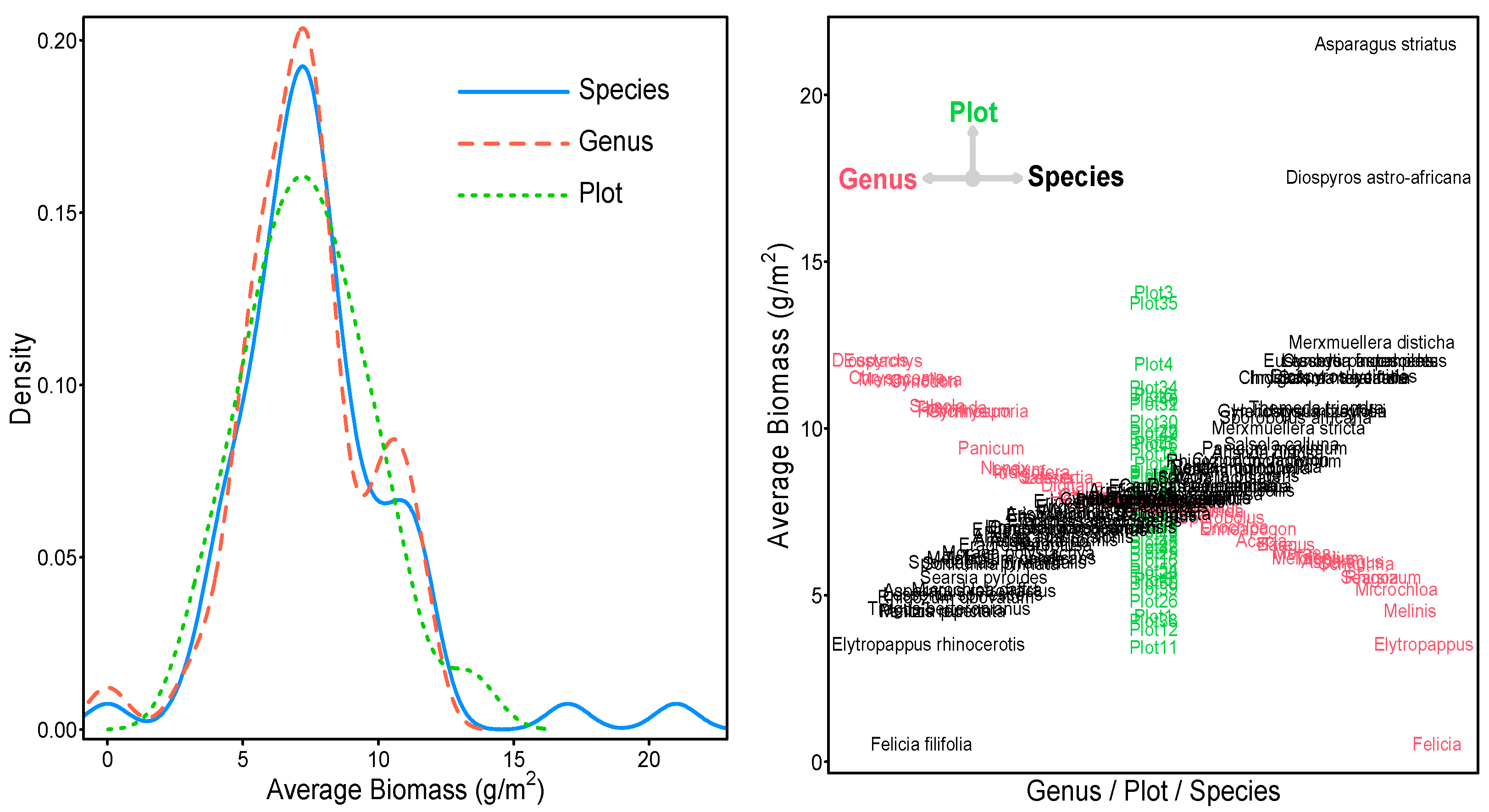
| Total | Genera | Species | Plot | |||
|---|---|---|---|---|---|---|
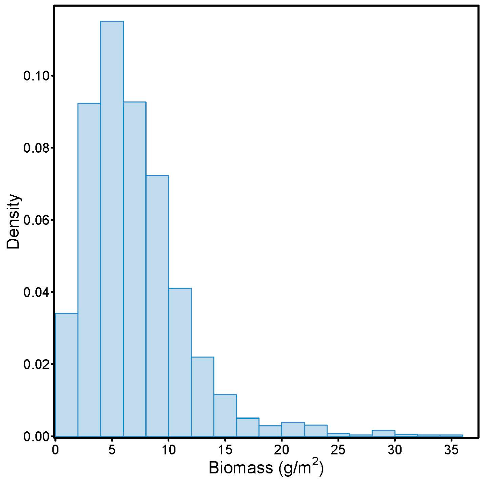
| Count | Biomass | 2594 | Average Biomass | 43 | 68 | 52 |
| Minimum | 0.00 | 0.00 | 0.00 | 2.90 | ||
| 25% Quantile | 4.00 | 5.87 | 6.08 | 5.85 | ||
| Median | 7.00 | 7.28 | 7.35 | 7.36 | ||
| 75% Quantile | 10.00 | 8.27 | 8.78 | 8.99 | ||
| Maximum | 36.00 | 11.52 | 21.00 | 13.54 | ||
| Mean | 7.45 | 7.29 | 7.70 | 7.45 | ||
| Std. Dev. | 4.55 | 2.36 | 3.03 | 2.35 | ||
| p-value | 0.0000 | 0.40 | 0.50 | 0.96 |
| Variable | n | Coeff. | p-Value * | 95% Conf. Int. | ||
|---|---|---|---|---|---|---|
| Lower | Upper | |||||
| Shannon index | 52 | −0.3623 | 0.5002 | −1.4339 | 0.7092 | |
| Aspect | ||||||
| East | 9 | Ref | Ref | Ref | Ref | |
| North | 7 | 1.5760 | 0.5002 | −3.0961 | 6.2480 | |
| North-east | 11 | 0.9920 | 0.6439 | −3.3036 | 5.2876 | |
| North-west | 6 | 1.5177 | 0.5480 | −3.5340 | 6.5694 | |
| South | 7 | 0.4668 | 0.9592 | −17.8360 | 18.7697 | |
| South-east | 2 | 0.0631 | 0.9739 | −3.8076 | 3.9338 | |
| South-west | 3 | 0.5944 | 0.9592 | −22.7120 | 23.9009 | |
| West | 7 | 1.1454 | 0.6439 | −3.8144 | 6.1052 | |
| Bulk density | 52 | 0.0388 | 0.9622 | −1.5957 | 1.6732 | |
| Cation exchange capacity | 52 | −0.0480 | 0.6103 | −0.2361 | 0.1401 | |
| Clay content | 52 | −0.0023 | 0.9622 | −0.0984 | 0.0938 | |
| Coarse fragments | 52 | −0.0044 | 0.9592 | −0.1764 | 0.1676 | |
| Nitrogen | 52 | −0.0042 | 0.9592 | −0.1682 | 0.1598 | |
| Annual mean rainfall | 52 | 0.0626 | 0.0585 | −0.0023 | 0.1275 | |
| Sand | 52 | 0.0077 | 0.9592 | −0.2952 | 0.3107 | |
| Silt | 52 | 0.0012 | 0.9622 | −0.0499 | 0.0524 | |
| Slope | 52 | 0.1392 | 0.4871 | −0.2601 | 0.5385 | |
| Soil organic carbon | 52 | 0.1935 | 0.1600 | −0.0790 | 0.4660 | |
| Annual mean temperature | 52 | −0.0275 | 0.9622 | −1.1845 | 1.1296 | |
| Vegetation unit | ||||||
| 1 | 12 | Ref | Ref | Ref | Ref | |
| 2–3 | 8 | 3.1008 | 0.0333 | 0.2564 | 5.9452 | |
| 4–5 | 14 | −0.0715 | 0.9622 | −3.0879 | 2.9449 | |
| 7–8 | 11 | 0.9058 | 0.6103 | −2.6463 | 4.4580 | |
| 9–11 | 7 | 2.3487 | 0.0993 | −0.4610 | 5.1584 | |
| Water pH | 52 | −0.0690 | 0.0385 | −0.1341 | −0.0038 | |
| Variable | DF | F-Value | p-Value * | |
|---|---|---|---|---|
| Aspect | 7 | 0.5672 | 0.9622 | 0.4365 |
| Vegetation unit | 4 | 4.5107 | 0.0385 | |
| Water pH | 1 | 8.2016 | 0.0416 |
Disclaimer/Publisher’s Note: The statements, opinions and data contained in all publications are solely those of the individual author(s) and contributor(s) and not of MDPI and/or the editor(s). MDPI and/or the editor(s) disclaim responsibility for any injury to people or property resulting from any ideas, methods, instructions or products referred to in the content. |
© 2023 by the authors. Licensee MDPI, Basel, Switzerland. This article is an open access article distributed under the terms and conditions of the Creative Commons Attribution (CC BY) license (https://creativecommons.org/licenses/by/4.0/).
Share and Cite
Munyai, N.; Ramoelo, A.; Adelabu, S.; Bezuidehout, H.; Sadiq, H. Effects of Environmental Factors on Plant Productivity in the Mountain Grassland of the Mountain Zebra National Park, Eastern Cape, South Africa. Ecologies 2023, 4, 749-761. https://doi.org/10.3390/ecologies4040049
Munyai N, Ramoelo A, Adelabu S, Bezuidehout H, Sadiq H. Effects of Environmental Factors on Plant Productivity in the Mountain Grassland of the Mountain Zebra National Park, Eastern Cape, South Africa. Ecologies. 2023; 4(4):749-761. https://doi.org/10.3390/ecologies4040049
Chicago/Turabian StyleMunyai, Nthabeliseni, Abel Ramoelo, Samuel Adelabu, Hugo Bezuidehout, and Hassan Sadiq. 2023. "Effects of Environmental Factors on Plant Productivity in the Mountain Grassland of the Mountain Zebra National Park, Eastern Cape, South Africa" Ecologies 4, no. 4: 749-761. https://doi.org/10.3390/ecologies4040049