
Numerical Investigation of Butterfly Valve Performance in Variable Valve Sizes, Positions and Flow Regimes

Department of Nuclear Engineering, University of New Mexico, Albuquerque, NM 87131, USA
*
Author to whom correspondence should be addressed.
J. Nucl. Eng. 2024, 5(2), 128-149; https://doi.org/10.3390/jne5020010
Submission received: 30 December 2023
/
Revised: 4 March 2024
/
Accepted: 17 April 2024
/
Published: 24 April 2024
Abstract
:Reliability and efficiency of valves are necessary for precise control and sufficient heat-flow to heat application plants for the integrated energy systems of nuclear power plants (NPPs). Strategic Management Analysis Requirement and Technology (SMART) valves’ ability to control flow and assess environmental parameters stands out for these requirements. Their ability to sustain the downstream flow rate, prevent reverse flow, and maintain pressure in the heat transport loop is much more efficient with the integration of sensors and intelligent algorithms. For assessing valve performance and monitoring, mechanical design and operating conditions are two important parameters. In this study, the butterfly valves of three different sizes are simulated with water and steam using STAR-CCM+ in various flow regimes and positions to analyze performance parameters to strategize an automated control system for efficiently balancing the heat–transport network. Also, flow behavior is studied using velocity and pressure fields for valve–body geometry optimization. It can be observed, through performance parameters, that the valves are suitable for operation between 30° and 90° positions with significantly low loss coefficients and high flow coefficients, and the performance parameters follow a certain pattern in both water and steam flow in each scenario.
1. Introduction
To address the various critical needs of water/steam flow controls and regulations, several types of valves are deployed and mounted upon the hydraulic networks and thermal hydraulics loops of commercial light water reactors (LWRs). Diverse kinds of valves serve different purposes, with the primary function being the regulation of downstream flow and the ability to turn on or off. Among these, butterfly valves stand out as one of the oldest and simplest candidates of flow control devices utilized across diverse liquid and gaseous transportation systems, particularly in situations where inlet velocity is high and minimal pressure drop is desired [1]. Characterized by their straightforward design, butterfly valves feature a disk-shaped valve body, distinguishing them for their simplicity. Operating such valves typically requires a quarter turn of the disk, rendering them more accessible to control and necessitating less maintenance compared to other valve types. This inherent simplicity contributes to their widespread use and practicality in various industrial applications. The widespread adoption of butterfly valves across various industries, power plants, and utility facilities can be attributed to the diverse range of sizes and variants available in the market. These variations, including no offset, single offset, double offset, and triple offset designs, cater to specific purposes and accommodate the different pressure ratings of the lines in which they are used. Butterfly valves have become indispensable in water supply, petroleum, and gas industries due to their versatility and adaptability to different operating conditions. Whether for managing flow in pipelines or controlling processes within industrial facilities, the availability of butterfly valves in various sizes and configurations ensures their applicability across a broad spectrum of industries and utility sectors.
Several R&D efforts have been put into butterfly valve performance characterization and optimization. Jeon et al. [2] studied the flow characteristics of single-disk and double-disk butterfly valves using FLUENT and compared the results in terms of the flow coefficient, loss coefficient, and pressure distribution in the flow. Sandalci et al. [3] worked on an experimental setup to investigate the effect of flow conditions and valve size on the performance of butterfly valves. The team employed the flow coefficient and loss coefficient to assess the performance of butterfly valves. Eom et al. [4] studied the butterfly valve performance as a flow controller and used two different configurations of valve body (solid blade and perforated blade). They executed the investigation by varying the blockade ratio and representing the data in terms of the loss coefficient. Toro and his team [5] performed a simulation study to investigate the performance of a 48-inch butterfly valve at different valve positions. They presented the performance factor with the loss coefficient and flow coefficient. They also compared their result with experimentally obtained values and compared the accuracy of the CFD tool in predicting the flow through the valve. Addy et al. [6] investigated the performance of a butterfly valve in the presence of compressible fluid. The team applied the sudden area enlargement theory to investigate the valve’s characteristics in the presence of the choked condition, stagnation pressure loss, and static pressure recovery. Song and his team [7] investigated a 1.8-meter (diameter) butterfly valve performance with ANSYS CFX and represented the result using the flow coefficient and the hydrodynamic torque. Leutwyler [8] performed a much more advanced study on butterfly valve performance. They investigated the performance of a butterfly valve in 45° and 70° positions, and, through a computational study, they measured the pressure contour, velocity contour, and the resultant force acting on the valve body. Morris [9] further extended the performance evaluation of butterfly valves by studying their performance in series and quantifying the pressure drop, mass flow coefficient, and upstream and downstream torque. So far, a comparative study of performance parameters in the full-range actuation of butterfly valves has yet to be performed. Without comparing performance data in the full range actuation, automated control strategy will lack the ability to predict the optimal amount of actuation.
There are more than 1500 valves in a typical 2 GW pressurized water reactor’s (PWR) primary loop, and 1.13 million valves deployed in the entire nuclear power plant’s (NPP) nuclear island, conventional island, and plant auxiliary facilities [10,11]. Until now, valves have been actuated either by manual or electronic actuation. Supervisions and synchronizations are performed in a manual manner (three-level supervision) [12]. Automating the hydraulic loop requires the creation of a valve network with automatic valve control mechanisms coordinated by intelligent algorithms. This system must be verified based on valve performance data for various valve positions and flow patterns to optimize valve actuation. In addition to this, thermal dispatch and power generation loads can be synchronized and balanced precisely. Automating an NPP’s hydraulic loop will help reduce operation costs by improving control and providing better safety for the plant and reducing human intervention.
Comparative analyses of valve performance play a crucial role in determining the mechanical compatibility and fitness of various valves in the thermal power system and designing the hydraulic networks (i.e., pipe size and layout). By analyzing performance metrics such as flow coefficients, pressure drop, and loss coefficients across different valves and configurations, engineers make informed decisions to minimize losses and mitigate impacts of design basis accidents, such as choked flow, cavitation, or overflow [13]. This theoretical simulation approach allows for fine-tuning hydraulic systems and ensuring optimal performance and reliability while minimizing energy consumption and operational risks. By selecting the most suitable valve size and configuration based on the thermal hydraulics performances of valves, engineers can achieve efficient flow regulation and identify potential issues that could threaten system integrities. This leads to more robust and cost-effective hydraulic systems in various industrial and utility applications.
This research aims to computationally analyze and compare the performance of butterfly valves across a wide variety of sizes at different flow rates at valve positions. This study seeks to visualize the flow fields through computational simulations and further provide a deeper understanding of their behavior. By systematically examining how these factors influence the performance of butterfly valves, researchers aim to gain insights into their efficiency, effectiveness, and operational characteristics under diverse operating conditions. This comprehensive investigation will enhance our understanding of valve performance and inform future design optimization scope and operational strategies for flow control in nuclear power sectors.
In this study, the butterfly valves with three different sizes (DN65, DN80, and DN100; DN being the nominal diameter) at six valve positions (15°, 30°, 45°, 60°, 75°, and 90°) are simulated with four velocities for both water and steam flow. Computational data are then used to observe various hydraulic phenomena, i.e., high-speed flow, flow stagnation, and vortex formation. The datasets of flow coefficients (Kv vs. Valve positions at different flow velocities) in this study can determine the optimal valve position from the flow Reynolds number. A cumulative control strategy can be employed to actuate the valve upstream, where the valve’s flow coefficient at upstream will be the cumulative flow coefficient of the valves at downstream. On the other hand, to control valves at downstream, a split-range control strategy can be used, where the downstream valve flow coefficients are determined by dividing the flow coefficient of the upstream valve according to the amount of flow rate through each valve. Correlating through flow coefficients, optimal valve positions can be calculated from the dataset obtained through this study. Hence, valves in a hydraulic network can be operated independently.
2. Computational Methodologies
The butterfly valves of modeling interest in this study are DN65, DN80, and DN100. The valve body geometry is slightly tapered from the stem to the edges, and the fillet is on both sides along the perimeter of the valve body. The whole flow domain has a total length of 20D (D is the inner diameter), where upstream has a 5D spacing and downstream has a 15D spacing. This spacing helps the downstream flow develop fully. For each case, the inner diameter is considered the characteristic diameter for Reynolds’ number. Four Reynolds numbers, Re = 400 in the laminar flow regime, Re = 4 k in transitional flow, Re = 40 k, and 400 k in turbulent flow, are simulated to characterize water flow behaviors. For steam flow simulation, Re = 4 k is in the transitional region, and Re = 40 k, 400 k, and 4000 k are in the turbulent region. Figure 1 shows the cross-section of the butterfly valve geometry used for the study.
To quantify the performance of butterfly valves, two parameters, the loss coefficient and flow coefficient, have been leveraged in this study to characterize the impacts of valve positions [5,14].
- a.
- Loss coefficient, K: Defines the ratio of pressure drop and the kinetic energy of the fluid as follows:
- b.
- Flow coefficient, Cv or Kv: Defines the flow capacity of a valve and corresponds to a unit pressure drop at a specific temperature. Cv is measured in imperial units, and Kv is measured in international standard units. They are related by the factor Cv = 1.16Kv. In this study, Kv is used to quantify the flow coefficients. The flow coefficient allows the flow capacities of valves of different sizes to be compared under a standard set of conditions. [15] The formula for the flow coefficient used in water flow is stated below:
The following formula is used [16] to compute the flow coefficient for simulating the steam flow across the valve body:
where, m is the flow rate in kg per hour, ΔP is the pressure drop across the valve body in bar, and is the specific volume of steam before the valve body.
Pressure drop is measured from the simulation at two points, where the upstream pressure is measured at 2.5D, and downstream pressure is measured at 10D downstream away from the valve body [3].
Velocity Limit Consideration: To minimize flow-induced damage (corrosion, erosion, cavitation) inside the pipe, the flow velocity is kept below a specific value. In our study, we use Kim’s criterion, stating that the maximum allowable velocity for water in NPPs is 6m/s [17]. In light of this, the maximum Reynolds number considered in this study is 400 k for water flow.
For the cases of steam flow, the maximum velocity limitation is 40 m/s, suggested by various sources [18]. Velocity in DN100 stays below this limit at Re = 4000 k, but DN80 and DN65 scenarios exhibit higher velocities (>40 m/s) at Re = 4000 k. To maintain the consistency of the results, velocities above 40 m/s are used in the simulations, but they are not recommended in practical scenarios.
3. Numerical Modeling and Verification
Boundary Conditions: In the simulations, the pipe and valve bodies are considered as no-slip walls. The inlet is defined as a uniform velocity inlet, and the outlet is a no-gradient pressure outlet. The length of the whole domain is such that the downstream flow can fully develop before the outlet. The turbulence intensity of the domain is kept at the default value of 10%. The simulated system is in adiabatic condition.
The software package used for the computation is STAR-CCM+. For defining physics simulation, the following settings are used to describe the physics from a relevant work of Y. Mu [19]. Table 1 lists the physics settings for the StarCCM+ to simulate water flow through butterfly valves.
Both models are compared by the indicator of the maximum velocity at a 60° position to quantify result differences.
4. Simulation Results and Analysis
A cylindrical element is placed around the valve body to capture the characteristics of the flow field, and volumetric refinement is applied after verifying grid independence.
4.1. Grid Independence Verification
The simulation is performed with various refinements ranging from 0.25 mm to 2 mm around the valve body to verify the grid independence. Grid sizes are calculated using the following equation:
Here, is the grid size, is the volume of the geometry, and is the number of cells in the simulation. The ratio of grid size r is calculated using the following equation:
where the and are the iterative values of the grid size. The ratio r is maintained greater than 1.3 and increases iteratively, as suggested by I.B. Celik. Four step sizes were considered as indicated by the same author in a different publication [20,21].
Table 3 lists the number of cells, grid size (calculated using Equation (4)), and the max velocity recorded during the simulation. A difference of 0.0202% is observed in the axial velocity produced by very fine mesh and fine mesh, while for the fine mesh and coarse mesh, it is 0.22%, and for the coarse mesh and very coarse mesh, it is 0.203%.
Considering the rate of change in maximum velocity in Table 3 and plot Figure 4, 0.5 mm mesh refinement is used in all the simulations in this study.
For meshing, surface remesher and polyhedral mesher are used. A cylinder body is used for volumetric mesh refinement around the valve body for the better visualization of the flow around the valve body, and the base mesh size is set to 5 mm with the default mesh growth rate. Figure 5a,b are the meshing of outer surface and valve body respectively.
4.2. Flow Field Visualization and Analysis for Water Flow
Velocity and pressure profiles are compared for DN100 valve size in four different Reynolds numbers at six valve positions. Table 4, Table 5, Table 6, Table 7, Table 8 and Table 9 present the velocity and pressure profiles for the water flow.
At narrow openings, 15° to 30° positions (Table 4 and Table 5), a localized high-velocity flow is observed, with a significant pressure difference between the upstream and downstream of the valve body. At 45° and 60° positions (Table 6 and Table 7), the highspeed zone is observed right behind (downstream) the valve body, which gradually merges downstream. Transitional flow (Re = 4 k) exhibited the most irregular pressure profile downstream in every valve position. This is because the transitional flow inherits laminar and turbulent flow characteristics. From 75° to 90° positions (Table 8 and Table 9), the velocity and pressure difference between the upstream and downstream diminishes significantly, and no eddy flow is observed downstream. The flow forms a continuous stream across the valve body, and the disappearance of the high-velocity zone is observed.
Stagnation region: In the laminar flow regime, a stagnant region is observed around the wall zone (around the valve body and near the pipe wall). As the velocity increases and the flow reaches the transitional regime, some stagnating region is observed near the wall upstream, and it is significantly smaller than that of the laminar flow. The stagnant zone formed on the upstream (front) of the valve body disappears gradually as the valve body transitions to a fully opened position. Figure 6 indicates the locations of stagnant region formations.
High-pressure stagnation region: This is observed at the front side (upstream) of the valve body and decreases significantly with increased velocity. Gradually, it shifts to the upstream, and resistance exerted on the flow becomes minimal. This stagnant region is much broader in smaller valve openings. As the opening widens, this zone diminishes in overall size, indicating that the resistance to flow becomes minimal with the opening of the valve.
Low-pressure stagnation region: This is observed downstream of the valve body. Up to a 60° position, this stagnation zone results in flow separation downstream. But from a 75° position, this region shrinks significantly. In laminar and transitional flow, the low-pressure zone adjacent to the downstream of the valve body displays a more significant disorder in the pressure profile than that of turbulent flow conditions.
Bernoulli effect region: The Bernoulli effect refers to an increase in flow velocity while transitioning from the high-pressure to the low-pressure zone. This phenomenon is observed when the flow is subjected to pass through a narrow opening. Observing the velocity and pressure profile of the 15° position, a very narrow high velocity stream is observed on the opening on both sides of the valve body. Up to a 60° position, this phenomenon is observed throughout all the flow regimes. In the pressure profile, the low-pressure zone is seen to be extruded to the upstream, resulting in a high-velocity stream. This high velocity flow merges downstream flow. From the 60° position, the localized jet converts to a continuous stream, and the Bernoulli effect diminishes, resulting in a drastic drop in maximum velocity in the flow field between 45° and 60° positions, which is calculated to be a 45% drop, on average, for every Reynolds number scenario. Figure 7a,b represent the pressure profile and velocity profile respectively for Bernoulli effect region.
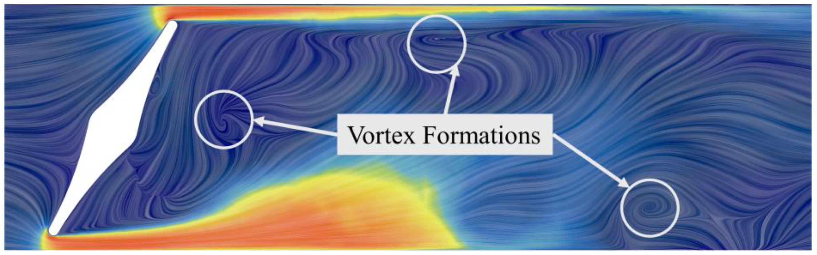
Formation of vortices: Vortex formation in flow is caused by localized rotation inside the flow caused by the localized high-velocity stream. In laminar, localized high velocity (for example, high velocity flow through the narrow opening) can cause boundary-layer separation, resulting in vortex formation. In the turbulent region, vortex formation is observed from a 15° to 45° position at Reynolds number values of 40k and 400k. However, these vortices diminish after this valve position and are not observed in wider openings. In 15° conditions, several vortices are observed approximately 6D downstream. At 30° and 45° positions, this region is observed to be shrunken, 4D and 3D, respectively. Vortex formation and swirls are not observed in wider valve positions. Figure 8 shows the vortices formed in such a scenario.
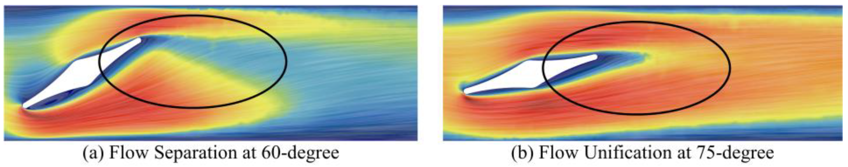
Flow separation and unification: Flow is separated by the low-pressure stagnation zone, created right behind (downstream) the valve–body diffusing downstream. From a 15° to 60° position, this diffusion zone widens, and flow separation is observed at the mid portion of the pipeline. After the 75° position, these two separate regions merge, and flow unification is observed, creating a unified stream. From the pressure profile, localized low-pressure zones are observed downstream adjacent to the valve body. Flow separation and irregularity in the pressure profile indicate the possibility of cavitation due to localized low-pressure zones. (Figure 9a) is the flow separation scenario and (Figure 9b) is the flow unification scenario represented in velocity profiles.
4.3. Comparison of Flow Field for DN65, DN80 and DN100 Valves at 60° Position for Water Flow
Table 10 lists the free stream velocity of the flow field. These velocities are calculated using the Reynolds numbers in each scenario.
Table 11 compares flow fields between DN65, DN80, and DN100. 60° positions are considered for this comparison as all hydraulic phenomena are observed from the widest to the narrowest valve openings in these flow conditions.
In the laminar flow regime for each size, a distinct high-velocity stream is observed at the midsection (core) of the flow field. Laminar flow is observed fully developed in approximately 3D downstream. In the case of transitional flow, this zone forms further downstream (approximately 10D), while it is not observed in turbulent flow cases.
High-velocity and low-pressure regions are observed on both sides of the valve body, transitioning the high-pressure flow downstream. In every scenario, the high-pressure zone is formed at the same position (upstream/front of the valve body).
Overall, DN80 and DN100 show very similar patterns in their velocity and pressure profiles. In the velocity profiles of DN65, a stagnant zone is observed on the region adjacent to the pipe wall downstream, which is not present in the DN80 and DN100. This stagnation is due to the narrow opening compared to the other two sizes, causing vortices downstream and resulting in a stagnant zone.
4.4. Performance Parameter Comparison for Kv and K Value for Water Flow
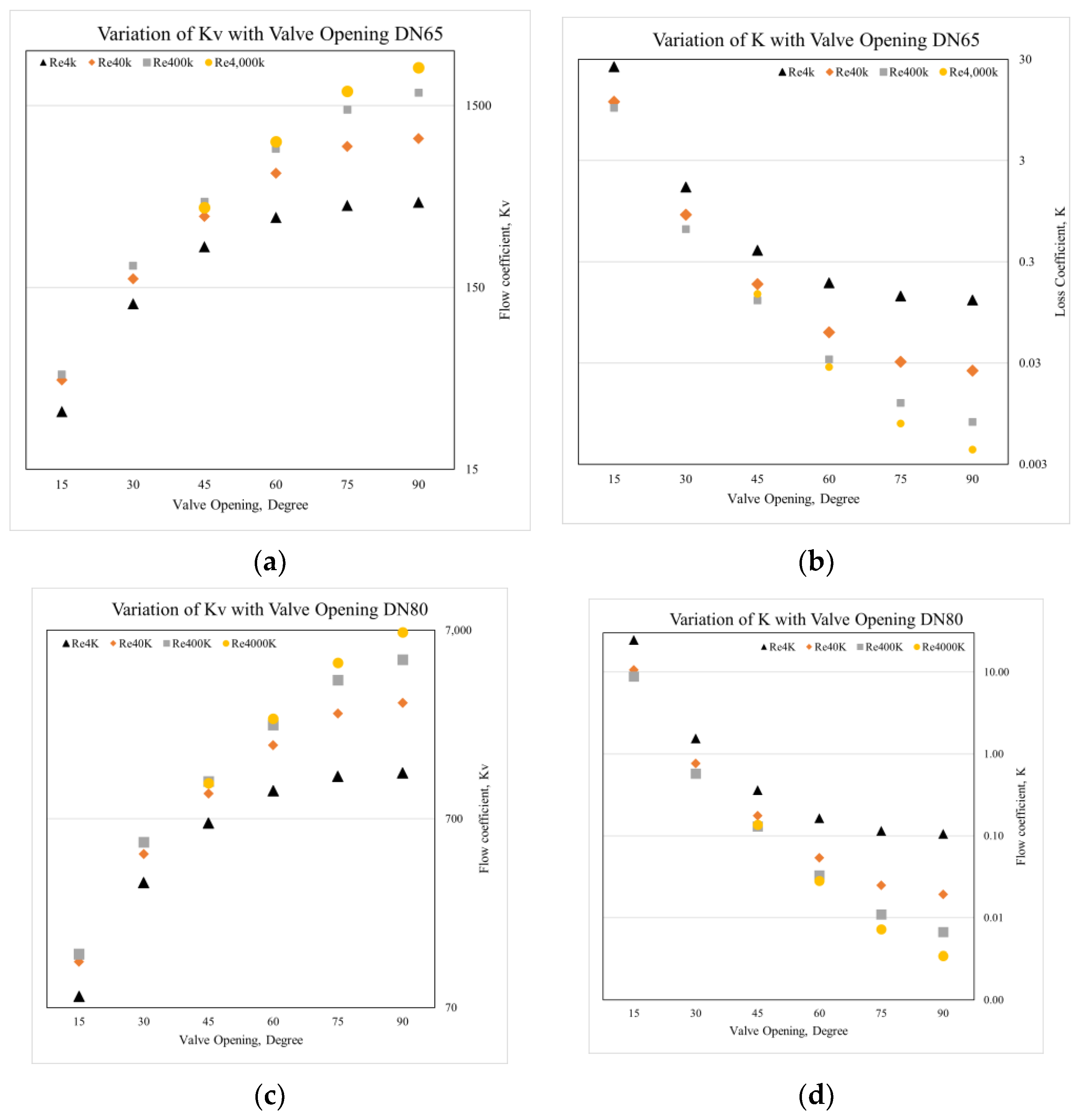
Figure 10a–f contain the flow coefficient (Kv) and loss coefficient for DN65, DN80, and DN100 in different valve positions. Figure 10a,c,e show the parametric trends of flow coefficient Kv with respect to valve positions, and Figure 10b,d,f show the parametric behaviors of the loss coefficient with respect to valve positions.
- Flow Coefficient (Kv) for Water Flow
Table 12 lists the flow coefficient data for all the water flow scenarios.
The typical pattern observed is that the flow coefficient value is higher in larger openings of the valve body. The loss coefficient increases over the progressive increase of the mass flow rate for a specific valve body position. Transitioning from laminar to transitional flow (Re = 400 to Re = 4 k), the change of loss coefficient is the highest in this dataset, at 27% in a 15° position and almost 100% in 75° and 90° positions. In turbulent flow, a coefficient peak value is observed, where the rate of increase is 19.42 per degree at Re = 400 k and 20.65 per degree at Re = 40 k in the DN100 valve. In laminar flow, the maximum rate of change is observed from a 45° to a 60° position. In transitional and turbulent flow conditions, this rate is maximum while transitioning from a 60° to 75° position, almost doubling from the prior range. In laminar flow, the rate of change drops after 60° and nearly levels at a fully opened condition. This high rate of change is due to localized jet formation, which indicates the difficulty of controlling the flow.
The rate of change of the flow coefficient per degree is vital while designing the control mechanisms. A high rate of change indicates the requirement for a much steadier and more precise actuation mechanism for the valve, as a slight change in valve actuation can significantly change the flow by rapidly increasing or decreasing the pressure drop.
- b.
- Loss Coefficient (K) for Water Fow
Table 13 lists the water flow’s loss coefficient (K) values across three butterfly valves.
Loss coefficients are maximum when the valve has the narrowest opening. Generally, this parameter is observed to be highest at a 15° position and lowest in the fully opened position. In a 30° position, the loss coefficient is less than 8% of the 15° position. This sharp drop in the loss coefficient indicates a significant reduction in the resistance of the valve on the flow while transitioning from a 15° to a 30° position. The loss coefficient drops as the valve reaches a fully opened position. From the 30° to 45° position, the loss coefficient drops 5.48/degree, on average, for the laminar flow, 3.32/degree for the transitional flow, and 2.48/degree for the turbulent region. From 60° to 90°, the rate of change drops below 1 in all the scenarios.
The rate of change also represents the slope of segments in the plots. Closely located values indicate that all three valve sizes follow a similar pattern while transitioning from a closed to fully opened condition. This also suggests that the loss coefficients depend on the valve body’s geometrical shape, as all three valves have the same geometrical features but only vary in size.
4.5. Simulating Steam Flow through Butterfly Valves
Steam flow at very low velocity (i.e., laminar flow) is not practical or efficient. For this reason, transitional flow (Re = 4 k) and turbulent flow (Re = 40 k, 400 k, 4000 k) are simulated. Table 14 lists the physics settings of StarCCM+ used for simulating steam flow.
The properties of the steam are taken at 543 K temperature and 7 MPa pressure, which is the environmental condition of a steam generator at the secondary loop. IAPWS-IF97 automatically determines steam’s physical properties according to the given temperature and pressure. At the stated condition, the density of steam is 36.557 kg/m3, which translates to a specific volume of 0.027 m3/kg.
4.6. Flow Field Visualization and Analysis for Steam Flow
Velocity and pressure profiles are compared for DN100 valve size in four different Reynolds numbers (two flow regimes) at six valve body positions. The upstream and downstream pressure difference becomes very high at higher velocity (Re = 400 k and 4000 k) and a narrow opening. It exhibits sonic velocity, causing unstable results with a very high value of simulation residuals. Due to this unreliability of the results, some scenarios (Re = 400 k at 15° and Re = 4000 k at 30° and 15° position) are omitted. Table 15, Table 16, Table 17, Table 18, Table 19 and Table 20 accommodate the velocity and pressure profile for the steam flow across butterfly valves.
Pressure drop across the valve body is significantly minor compared to the water flow, as the density of steam is considerably lower. For this reason, vortex formation is not observed downstream as much as in the water flow. Only the 15° and 30° positions (Table 15 and Table 16) exhibited vortex formation, implying a higher pressure drop. A significant pressure drop is observed downstream of the valve body from the 15° to 30° positions. This difference is significantly lower from the 45° to 90° positions (Table 17, Table 18, Table 19 and Table 20).
Water flow and steam flow across the valve produce a significantly similar pattern. The stagnation zone is significantly prominent for the steam flow and is located by the wall. The cross-sectional area of the high-pressure stagnation zone is more petite and mostly located upstream of the valve body, similar to the water flow. The low-pressure stagnation zone is observed downstream. Bernoulli effect regions are smaller due to the flowing medium’s lower pressure and density. Jet-like flow is observed in smaller openings (15° and 30° positions). Flow separation and unification are more significant in the steam flow. From the 45° position, flow unification is observed, and the pressure drop is significantly reduced, but from the 15° to 45° position, some swirlings are observed in the velocity profile.
4.7. Comparison of Flow for DN65, DN80 and DN100 Valves at 60° Position for Steam Flow
Velocities listed in Table 21 are calculated from the steam density and specified Reynolds’ numbers. For comparison purposes, velocities more than the allowable limit (40 m/s) are considered. Table 22 accommodates the comparative visualization of the flow and pressure fields of DN65, DN80 and DN100.
DN80 and DN100 exhibit similar patterns in the flow field in all the compared scenarios. The area of the Bernoulli effect region is similar to downstream. For DN65 (Re = 400 k and 4000 k), a prominent stagnant zone is observed behind the Bernoulli effect zone due to the narrow opening causing localized vortices and stagnation, which is not observed in DN80 and DN100. All scenarios show flow separation downstream, but the stagnant zone around the valve body is more significant in DN65. Re = 4 k and 40 k have a high-velocity stream at the middle (core) and stagnant zone adjacent to the pipe wall. This core region indicates the recovery and unification of flow after the valve body scrambles the stream. The formation of high- and low-pressure stagnation regions is similar in all the scenarios.
4.8. Performance Parameter Comparison for Kv and K Value for Steam Flow
Table 23 and Table 24 list out the flow coefficients and loss coefficients data, respectively, for steam flow. Figure 11 shows the plots of the flow coefficients (Figure 11a,c,e) and loss coefficients (Figure 11b,d,f) observed. Numerical values of flow coefficients and loss coefficients are listed in Table 23 and Table 24.
- a.
- Flow Coefficient (Kv) for Steam Flow
Flow coefficients for steam flow are significantly higher than those of water flow. For example, DN100 at Re = 400 k, steam flow results in a 4 times higher value of flow coefficients for water flow at Re = 400 k. The transition flow exhibits significantly lower flow coefficients than water flow. For water flow in the DN100 valve, the ratio of flow coefficients at transitional flow (Re = 4 k) and turbulent flow (Re = 400 k) is 2, whereas, for steam flow, this ratio is almost 8, indicating significantly better performance for steam flow with the same valve. This is due to the lower pressure drop across the valve body in steam flow. Figure 11a,c,e show the plot of flow coefficients for steam flow.
- b.
- Loss Coefficient (K) for Steam Flow
Loss coefficients are non-dimensional pressure drops, and the steam flow exhibits a lower pressure drop across the valve compared to the water flow. For example, the coefficient for DN65 at Re = 4 k is about 55 times lower than that of the water flow. From a fully opened (90° position) to a 30° position, the loss coefficients are significantly lower in value (below 1) for the steam flow. This indicates easier flow control with butterfly valves compared to the water flow. Loss coefficients range from 40 to 105 at a 30° position for the water flow, significantly more than the steam flow. Figure 11b,d,f shows the plot of loss coefficients for the steam flow.
5. Conclusions
This computational study compares butterfly valves of three different sizes in different flow regimes and valve opening angles in the steam and water flow. Performance parameter data obtained through this study is in good agreement with the performance parameters obtained by other research works and industry standards.
This study concludes that the butterfly valves are suitable flow controllers from a 30° position to a 90° position (fully opened). In most water flow scenarios, the loss coefficients are below 100 when the valve position is above 15°, which is an acceptable value for a hydraulic loop. Our simulation results demonstrate that the loss coefficients drop significantly (approximately 90%) from a 15° to a 30° position. For the steam flow, a similar decline in the loss coefficient is observed between the 15° to 30° positions. Therefore, the 30° to 90° position is suitable for actuation and flow control.
Butterfly valves exert almost no resistance in fully open conditions. From the flow coefficient values, it can be concluded that higher velocity and a broader opening are better for flow performance with a low-pressure drop. The turbulent flow is undoubtedly the most desirable condition as a more flowing medium can flow through the pipeline for water and steam. From the data of laminar and transitional flow conditions, it is observed that the change in flow coefficients is much even, with a minor shift in coefficients per degree. In turbulent regimes, the rate of change per degree is very high, with a steep gain of flow coefficient as the opening widens. This requires an energy-consuming actuation method to control the valve in this flow regime precisely. For an efficient control strategy, a combination of pump speed and valve actuation should be introduced to minimize pressure spike buildup in upstream and localized high-speed jet formation around the valve body. This strategy will significantly reduce the torque requirement for motorized valve actuation, resulting in easier valve actuation.
Finally, comparative performance data can be utilized to strategize the automated control of the hydraulic loop with the butterfly valve. The plots obtained through this study are Kv vs. Valve positions. If the flow rate is specified for downstream, the corresponding flow coefficients of downstream valves can be utilized to interpret the required valve position for the valve upstream. The flow coefficient upstream will be the cumulative flow coefficient downstream. On the other hand, the downstream valve can be actuated with a split range control strategy, where the flow coefficient at upstream will be divided proportionally among the valves downstream according to the amount of flow through each of the valves, and then translated to the corresponding valve position data from the obtained results of this study.
For future research, more diverse types of data (i.e., pressure, density, the temperature of the medium) can be introduced to this control strategy, which will significantly improve the safety and precision of the system.
Author Contributions
Conceptualization, A.B. and M.C.; methodology, A.B.; software, M.C.; validation, A.B.; formal analysis, A.B.; investigation, A.B.; resources, M.C.; data curation, A.B.; writing—original draft preparation, A.B.; writing—review and editing, M.C. and M.H.; visualization, A.B., M.H. and M.C.; supervision, M.C.; project administration, M.C.; funding acquisition, M.C. All authors have read and agreed to the published version of the manuscript.
Funding
This research was funded by the U.S. Department of Energy, grant number DE-NE0009278.
Data Availability Statement
The data presented in this study are available upon request.
Acknowledgments
This report was prepared as an account of work sponsored by an agency of the United States Government. Neither the United States Government nor any agency thereof, nor any of their employees, makes any warranty, express or implied, or assumes any legal liability or responsibility for the accuracy, completeness, or usefulness of any information, apparatus, product, or process disclosed, or represents that its use would not infringe privately owned rights. Reference herein to any specific commercial product, process, or service by trade name, trademark, manufacturer, or otherwise does not necessarily constitute or imply its endorsement, recommendation, or favoring by the United States Government or any agency thereof. The views and opinions of authors expressed herein do not necessarily state or reflect those of the United States Government or any agency thereof.
Conflicts of Interest
The authors declare no conflicts of interest. The funders had no role in the design of the study; in the collection, analyses, or interpretation of data; in the writing of the manuscript; or in the decision to publish the results.
References
- Naragund, P.S.; Nasi, V.B.; Kulkarni, G.V. Study of Hydrodynamic Torque of Double Offset Butterfly Valve Disc through Experiment and CFD Analysis. Int. J. Veh. Struct. Syst. (IJVSS) 2021, 13, 76. [Google Scholar] [CrossRef]
- Jeon, S.Y.; Yoon, J.Y.; Shin, M.S. Flow characteristics and performance evaluation of butterfly valves using numerical analysis. In IOP Conference Series: Earth and Environmental Science; IOP Publishing: Bristol, UK, 2010; Volume 12, p. 012099. [Google Scholar]
- Sandalci, M.; Mançuhan, E.; Alpman, E.; Küçükada, K. Effect of the flow conditions and valve size on butterfly valve performance. J. Therm. Sci. Technol. 2010, 30, 103–112. [Google Scholar]
- Eom, K. Performance of butterfly valves as a flow controller. J. Fluids Eng. 1988, 110, 16–19. [Google Scholar] [CrossRef]
- Del Toro, A.; Johnson, M.C.; Spall, R.E. Computational fluid dynamics investigation of butterfly valve performance factors. J. Am. Water Works Assoc. 2015, 107, E243–E254. [Google Scholar] [CrossRef]
- Addy, A.L.; Morris, M.J.; Dutton, J.C. An investigation of compressible flow characteristics of butterfly valves. J. Fluids Eng. 1985, 107, 512–517. [Google Scholar] [CrossRef]
- Guan Song, X.; Park, Y.C. Numerical analysis of butterfly valve-prediction of flow coefficient and hydrodynamic torque coefficient. In Proceedings of the World Congress on Engineering and Computer Science (WCECS 2007), San Francisco, CA, USA, 24–26 October 2007; pp. 24–26. [Google Scholar]
- Leutwyler, Z.; Dalton, C. A CFD study of the flow field, resultant force, and aerodynamic torque on a symmetric disk butterfly valve in a compressible fluid. J. Press. Vessel Technol. 2008, 130, 021302. [Google Scholar] [CrossRef]
- Morris, M.J.; Dutton, J.C. The performance of two butterfly valves mounted in series. J. Fluids Eng. 1991, 113, 419–423. [Google Scholar] [CrossRef]
- Qian, J.Y.; Hou, C.W.; Mu, J.; Gao, Z.X.; Jin, Z.J. Valve core shapes analysis on flux through control valves in nuclear power plants. Nucl. Eng. Technol. 2020, 52, 2173–2182. [Google Scholar] [CrossRef]
- Gate Valves Used for Nuclear Plant. Perfect Valve. Available online: https://perfect-valve.com/gate-valves-used-for-nuclear-plant/ (accessed on 2 July 2023).
- Agarwal, V.; Buttles, J.W.; Beaty, L.H.; Naser, J.; Hallbert, B.P. Wireless online position monitoring of manual valve types for plant configuration management in nuclear power plants. IEEE Sens. J. 2016, 17, 311–322. [Google Scholar] [CrossRef]
- What Is Valve Flow Coefficient (Cv)? Kimray. Available online: https://kimray.com/training/what-valve-flow-coefficient-cv (accessed on 2 July 2023).
- Chern, M.J.; Wang, C.C.; Ma, C.H. Performance test and flow visualization of ball valve. Exp. Therm. Fluid Sci. 2007, 31, 505–512. [Google Scholar] [CrossRef]
- Crabtree, M.A. The Concise Valve Handbook, Volume I: Sizing and Construction; Momentum Press: New York, NY, USA, 2018. [Google Scholar]
- Steam Control Valves—Calculate Flow Factor, Kv. The Engineering Toolbox. Available online: https://www.engineeringtoolbox.com/control-valves-steam-d_264.html (accessed on 26 December 2023).
- Kim, S. Maximum allowable fluid velocity and concern on piping stability of ITER tokamak cooling water system. Fusion Eng. Des. 2021, 162, 112049. [Google Scholar] [CrossRef]
- Recommended Velocities in Steam Systems. The Engineering Toolbox. Available online: https://www.engineeringtoolbox.com/flow-velocity-steam-pipes-d_386.html (accessed on 27 December 2023).
- Mu, Y.; Liu, M.; Ma, Z. Research on the measuring characteristics of a new design butterfly valve flowmeter. Flow Meas. Instrum. 2019, 70, 101651. [Google Scholar] [CrossRef]
- Celik, I.B.; Ghia, U.; Roache, P.J.; Freitas, C.J. Procedure for estimation and reporting of uncertainty due to discretization in CFD applications. J. Fluids Eng. Trans. ASME 2008, 130, 078001. [Google Scholar] [CrossRef]
- Celik, I.B.; Ma, Z.; Benyahia, S. Discretization error estimation in transient flow simulations. In Fluids Engineering Division Summer Meeting; American Society of Mechanical Engineers: New York, NY, USA, 2016; Volume 50282, p. V01AT06A005. [Google Scholar]
Figure 1.
Cross-section of the butterfly valve.

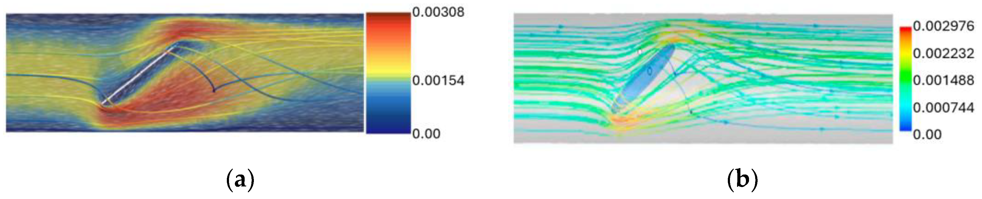
Figure 2.
At Re = 150: (a) our model; (b) simulation model by Y. Mu et al. [19].
Figure 2.
At Re = 150: (a) our model; (b) simulation model by Y. Mu et al. [19].

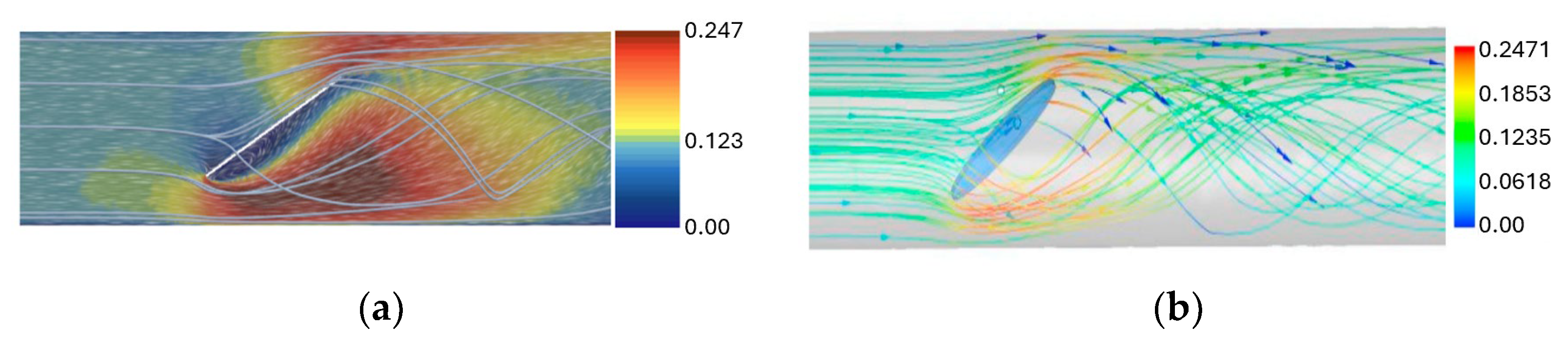
Figure 3.
At Re = 15 k: (a) our model; (b) simulation model by Mu et al. [19].
Figure 3.
At Re = 15 k: (a) our model; (b) simulation model by Mu et al. [19].

Figure 4.
Grid independence verification.

Figure 5.
Meshing and refinement on the (a) outside and (b) inside.

Figure 6.
Stagnation regions.

Figure 7.
Bernoulli effect region.

Figure 8.
Vortex formations.

Figure 9.
Flow separation and unification.

Figure 10.
Performance parameter plots for water flow: (a,b) DN65—K, (c) DN80—Kv, (d) DN80—K, (e) DN100—Kv, (f) DN100—K.
Figure 10.
Performance parameter plots for water flow: (a,b) DN65—K, (c) DN80—Kv, (d) DN80—K, (e) DN100—Kv, (f) DN100—K.


Figure 11.
Performance parameter plots for steam flow: (a) DN65—Kv, (b) DN65—K, (c) DN80—Kv, (d) DN80—K, (e) DN100—Kv, (f) DN100—K.
Figure 11.
Performance parameter plots for steam flow: (a) DN65—Kv, (b) DN65—K, (c) DN80—Kv, (d) DN80—K, (e) DN100—Kv, (f) DN100—K.


Table 1.
Physics settings for STAR-CCM+ (Water Flow).
| For the Laminar Flow Regime | For Turbulent and Transitional Flow Regime |
|---|---|
|
|
|
|
|
|
|
|
|
|
|
|
|
|
| |
| |
| |
|
Table 2.
Simulation parameters by Mu et al. [19].
Table 2.
Simulation parameters by Mu et al. [19].
| Parameter | Value |
|---|---|
| Density of liquid | 998.2 kg/m3 |
| Dynamic viscosity | 0.001004 Pa s |
| Internal pipe diameter | 0.15 m |
| Valve position | 60° |
| Valve geometry | 2 mm in thickness with round fillets along both edges |
| Reynolds numbers used for validation | 150 (Laminar, V = 0.0010048 m/s) 15k (Turbulent, V = 0.10048 m/s) |
Table 3.
Mesh refinement data.
| Refinement (mm) | Cells | Max Velocity (m/s) | Grid Size (h) | R (= hcoarse/hfine) |
|---|---|---|---|---|
| 0.25 (Very Fine) | 9,961,163 | 0.24699 | 0.001525215 | 1 |
| 0.5 (Fine) | 2,591,976 | 0.24694 | 0.002389044 | 1.566365192 |
| 1 (Coarse) | 882,503 | 0.24639 | 0.003421336 | 1.432094231 |
| 2 (Very Coarse) | 399,255 | 0.24589 | 0.004456744 | 1.302632599 |
Table 4.
Flow field for 15° valve position.
| Re | Velocity Profile | Pressure Profile |
|---|---|---|
| 400 |  |  |
| 4 k |  |  |
| 40 k |  |  |
| 400 k |  |  |
Table 5.
Flow field for 30° valve position.
| Re | Velocity Profile | Pressure Profile |
|---|---|---|
| 400 |  |  |
| 4 k |  |  |
| 40 k |  |  |
| 400 k |  |  |
Table 6.
Flow field for 45° valve position.
| Re | Velocity Profile | Pressure Profile |
|---|---|---|
| 400 |  |  |
| 4 k |  |  |
| 40 k |  |  |
| 400 k |  |  |
Table 7.
Flow field for 60° valve position.
| Re | Velocity Profile | Pressure Profile |
|---|---|---|
| 4 k |  |  |
| 40 k |  |  |
| 400 k |  |  |
| 4000 k |  |  |
Table 8.
Flow field for 75° valve position.
| Re | Velocity Profile | Pressure Profile |
|---|---|---|
| 400 |  |  |
| 4 k |  |  |
| 40 k |  |  |
| 400 k |  |  |
Table 9.
Flow field for 90° valve position.
| Re | Velocity Profile | Pressure Profile |
|---|---|---|
| 400 |  |  |
| 4 k |  |  |
| 40 k |  |  |
| 400 k |  |  |
Table 10.
Velocity for different scenarios.
| Re | DN65 | DN80 | DN100 |
|---|---|---|---|
| 400 | 0.005685 m/s | 0.004573 m/s | 0.003563 m/s |
| 4 k | 0.05685 m/s | 0.04573 m/s | 0.03563 m/s |
| 40 k | 0.5685 m/s | 0.4573 m/s | 0.3563 m/s |
| 400 k | 5.685 m/s | 4.573 m/s | 3.563 m/s |
Table 11.
Comparative visualization of velocity and pressure profile in three valve sizes for water flow.
Table 11.
Comparative visualization of velocity and pressure profile in three valve sizes for water flow.
| Velocity Profile | |||
|---|---|---|---|
| Re | DN65 | DN80 | DN100 |
| 400 |  |  |  |
 | |||
| 4 k |  |  |  |
 | |||
| 40 k |  |  |  |
 | |||
| 400 k |  |  |  |
 | |||
| Pressure Profile | |||
| 400 |  |  |  |
 | |||
| 4 k |  |  |  |
 | |||
| 40 k |  |  |  |
 | |||
| 400 k |  |  |  |
 | |||
Table 12.
Flow coefficients Kv for all scenarios (water flow).
| Size | Re | 90° | 75° | 60° | 45° | 30° | 15° |
|---|---|---|---|---|---|---|---|
| DN65 | 400 | 73.41 | 68.83 | 53.43 | 33.07 | 15.38 | 4.20 |
| 4 k | 151.26 | 128.51 | 82.07 | 43.35 | 19.61 | 5.43 | |
| 40 k | 216.47 | 169.75 | 98.29 | 49.05 | 21.99 | 6.03 | |
| 400 k | 284.1 | 200.47 | 106.67 | 51.52 | 22.79 | 6.30 | |
| DN80 | 400 | 124.91 | 115.75 | 86.15 | 51.59 | 23.56 | 6.46 |
| 4 k | 246.07 | 205.48 | 127.87 | 67.31 | 30.27 | 8.91 | |
| 40 k | 350.38 | 273.43 | 155.83 | 77.85 | 34.99 | 10.48 | |
| 400 k | 465.99 | 327.30 | 171.76 | 82.68 | 36.68 | 10.92 | |
| DN100 | 400 | 263.65 | 232.65 | 158.30 | 68.46 | 37.42 | 11.30 |
| 4 k | 490.40 | 390.37 | 220.94 | 111.73 | 51.75 | 15.60 | |
| 40 k | 684.98 | 518.85 | 271.23 | 133.73 | 59.25 | 18.55 | |
| 400 k | 903.89 | 612.61 | 302.84 | 142.35 | 62.22 | 19.50 |
Table 13.
Loss coefficients K for all scenarios (water flow).
| Size | Re | 90° | 75° | 60° | 45° | 30° | 15° |
|---|---|---|---|---|---|---|---|
| DN65 | 400 | 4.59 | 5.22 | 8.67 | 22.62 | 104.63 | 1400.80 |
| 4 k | 1.08 | 1.50 | 3.67 | 13.16 | 64.37 | 839.42 | |
| 40 k | 0.53 | 0.86 | 2.56 | 10.28 | 51.15 | 680.11 | |
| 400 k | 0.31 | 0.62 | 2.17 | 9.32 | 47.64 | 623.24 | |
| DN80 | 400 | 3.79 | 4.41 | 7.96 | 22.20 | 106.47 | 1413.94 |
| 4 k | 0.98 | 1.40 | 3.61 | 13.04 | 64.48 | 744.97 | |
| 40 k | 0.48 | 0.79 | 2.43 | 9.75 | 48.26 | 537.91 | |
| 400 k | 0.27 | 0.55 | 2.00 | 8.64 | 43.91 | 495.41 | |
| DN100 | 400 | 2.31 | 2.96 | 6.40 | 34.20 | 114.45 | 1256.43 |
| 4 k | 0.67 | 1.05 | 3.28 | 12.84 | 59.86 | 658.39 | |
| 40 k | 0.34 | 0.60 | 2.18 | 8.96 | 45.66 | 466.01 | |
| 400 k | 0.20 | 0.43 | 1.75 | 7.91 | 41.39 | 421.61 |
Table 14.
Steam flow physics settings.
| For Turbulent Flow Regime |
|---|
|
Table 15.
Flow field for 15° valve position.
| Re | Velocity Profile | Pressure Profile |
|---|---|---|
| 4 k |  |  |
| 40 k |  |  |
Table 16.
Flow field for 30° valve position.
| Re | Velocity Profile | Pressure Profile |
|---|---|---|
| 4 k |  |  |
| 40 k |  |  |
| 400 k |  |  |
Table 17.
Flow field for 45° valve position.
| Re | Velocity Profile | Pressure Profile |
|---|---|---|
| 4 k |  |  |
| 40 k |  |  |
| 400 k |  |  |
| 4000 k |  |  |
Table 18.
Flow field for 60° valve position.
| Re | Velocity Profile | Pressure Profile |
|---|---|---|
| 4 k |  |  |
| 40 k |  |  |
| 400 k |  |  |
| 4000 k |  |  |
Table 19.
Flow field for 75° valve position.
| Re | Velocity Profile | Pressure Profile |
|---|---|---|
| 4 k |  |  |
| 40 k |  |  |
| 400 k |  |  |
| 4000 k |  |  |
Table 20.
Flow field for 90° valve position.
| Re | Velocity Profile | Pressure Profile |
|---|---|---|
| 4 k |  |  |
| 40 k |  |  |
| 400 k |  |  |
| 4000 k |  |  |
Table 21.
Velocity for different scenarios for steam flow.
| Re | DN65 | DN80 | DN100 |
|---|---|---|---|
| 4 k | 0.0386 m/s | 0.0505 m/s | 0.063 m/s |
| 40 k | 0.386 m/s | 0.505 m/s | 0.63 m/s |
| 400 k | 3.857 m/s | 5.05 m/s | 6.277 m/s |
| 4000 k | 38.57 m/s | 50.5 m/s | 62.77 m/s |
Table 22.
Comparative visualization of velocity and pressure profile in three valve sizes for steam flow.
Table 22.
Comparative visualization of velocity and pressure profile in three valve sizes for steam flow.
| Velocity Profile | |||
|---|---|---|---|
| Re | DN65 | DN80 | DN100 |
| 4 k |  |  |  |
 | |||
| 40 k |  |  |  |
 | |||
| 400 k |  |  |  |
 | |||
| 4000 k |  |  |  |
 | |||
| Pressure Profile | |||
| 4 k |  |  |  |
 | |||
| 40 k |  |  |  |
 | |||
| 400 k |  |  |  |
 | |||
| 4000 k |  |  |  |
 | |||
Table 23.
Flow coefficients Kv for all scenarios (steam flow).
| Size | Re | 90° | 75° | 60° | 45° | 30° | 15° |
|---|---|---|---|---|---|---|---|
| DN65 | 4 k | 441.93 | 423.39 | 363.92 | 251.45 | 122.37 | 31.17 |
| 40 k | 988.73 | 893.49 | 638.02 | 368.88 | 167.65 | 46.42 | |
| 400 k | 1767.17 | 1423.73 | 868.75 | 443.88 | 197.70 | ||
| 4000 k | 2425.17 | 1798.01 | 947.71 | 412.07 | |||
| DN80 | 4 k | 936.47 | 896.45 | 752.75 | 506.84 | 244.67 | 61.35 |
| 40 k | 2199.11 | 1930.57 | 1311.13 | 727.01 | 347.67 | 93.47 | |
| 400 k | 3728.51 | 2905.90 | 1682.11 | 843.73 | 401.58 | ||
| 4000 k | 5209.15 | 3590.22 | 1817.75 | 825.39 | |||
| DN100 | 4 k | 781.55 | 1013.02 | 1078.04 | 378.50 | 238.66 | 84.47 |
| 40 k | 2044.54 | 2477.89 | 1729.54 | 875.85 | 450.70 | 120.44 | |
| 400 k | 3996.51 | 3756.69 | 2295.40 | 1142.55 | 516.81 | ||
| 4000 k | 5840.65 | 4798.33 | 2548.59 | 1183.42 |
Table 24.
Loss coefficients K for all scenarios (Steam flow).
| Size | Re | 90° | 75° | 60° | 45° | 30° | 15° |
|---|---|---|---|---|---|---|---|
| DN65 | 4 k | 0.13 | 0.14 | 0.19 | 0.39 | 1.64 | 25.27 |
| 40 k | 0.03 | 0.03 | 0.06 | 0.18 | 0.87 | 11.39 | |
| 400 k | 0.01 | 0.01 | 0.03 | 0.12 | 0.63 | ||
| 4000 k | 0.00418 | 0.01 | 0.03 | 0.14 | |||
| DN80 | 4 k | 0.18 | 0.20 | 0.28 | 0.62 | 2.66 | 42.27 |
| 40 k | 0.03 | 0.04 | 0.09 | 0.30 | 1.32 | 18.21 | |
| 400 k | 0.01 | 0.02 | 0.06 | 0.22 | 0.99 | ||
| 4000 k | 0.01 | 0.01 | 0.05 | 0.23 | |||
| DN100 | 4 k | 0.28 | 0.17 | 0.15 | 1.21 | 3.05 | 24.38 |
| 40 k | 0.04 | 0.03 | 0.06 | 0.23 | 0.86 | 11.99 | |
| 400 k | 0.01 | 0.01 | 0.03 | 0.13 | 0.65 | ||
| 4000 k | 0.01 | 0.01 | 0.03 | 0.12 |
Disclaimer/Publisher’s Note: The statements, opinions and data contained in all publications are solely those of the individual author(s) and contributor(s) and not of MDPI and/or the editor(s). MDPI and/or the editor(s) disclaim responsibility for any injury to people or property resulting from any ideas, methods, instructions or products referred to in the content. |
© 2024 by the authors. Licensee MDPI, Basel, Switzerland. This article is an open access article distributed under the terms and conditions of the Creative Commons Attribution (CC BY) license (https://creativecommons.org/licenses/by/4.0/).
Share and Cite
MDPI and ACS Style
Bairagi, A.; He, M.; Chen, M. Numerical Investigation of Butterfly Valve Performance in Variable Valve Sizes, Positions and Flow Regimes. J. Nucl. Eng. 2024, 5, 128-149. https://doi.org/10.3390/jne5020010
AMA Style
Bairagi A, He M, Chen M. Numerical Investigation of Butterfly Valve Performance in Variable Valve Sizes, Positions and Flow Regimes. Journal of Nuclear Engineering. 2024; 5(2):128-149. https://doi.org/10.3390/jne5020010
Chicago/Turabian StyleBairagi, Anutam, Mingfu He, and Minghui Chen. 2024. "Numerical Investigation of Butterfly Valve Performance in Variable Valve Sizes, Positions and Flow Regimes" Journal of Nuclear Engineering 5, no. 2: 128-149. https://doi.org/10.3390/jne5020010