
Comparison of Inductive Thermography and Computer Tomography Results for Short Surface Cracks †


Department Product Engineering, University of Leoben, 8700 Leoben, Austria
†
Presented at the 17th International Workshop on Advanced Infrared Technology and Applications, Venice, Italy, 10–13 September 2023.
Eng. Proc. 2023, 51(1), 36; https://doi.org/10.3390/engproc2023051036
Published: 14 November 2023
(This article belongs to the Proceedings of The 17th International Workshop on Advanced Infrared Technology and Applications)
Abstract
:Inductive thermography is a non-destructive testing method, whereby the workpiece to be inspected is slightly heated by a short inductive heating pulse. An infrared camera records the surface temperature during and after the heating pulse. As defects influence the induced eddy current distribution and the heat flow, they become highly visible in the evaluated infrared images. The deeper a crack is, the greater the obstacle it represents. In Inconel welded samples, short surface cracks (length 0.3–2 mm) were created using a so-called Varestraint test machine. The samples were inspected via inductive thermography and computer tomography (CT). Additional finite element simulations were calculated in order to model the thermography experiments. The comparison of the thermographic, CT and simulation results shows how the thermographic signal of a defect depends on its geometry. This information can be used for calibration to estimate the crack properties based on the thermographic inspection.
1. Introduction
In the case of inductive thermography, the workpiece is heated by a short induction heating pulse, usually with a duration between 50 ms and 1 s, and an infrared camera records the surface temperature. As surface cracks disturb the eddy current distribution and also the heat flow, the defects can be well recognized in the infrared images. Therefore, inductive thermography as a non-destructive inspection method is used more and more often in industry in order to detect surface cracks in a quick and contactless way [1,2,3,4,5].
An additional advantage of this inspection technique is that it makes it not only possible to localize the defects but also gives information about depth. In order to prove this statement, additional computer tomography (CT) measurements were carried out on the samples to determine the depth of the cracks. In a further step, the CT results were combined with the inductive thermography results to investigate their crack depth dependency.
2. Finite Element Simulations
Finite element simulations (FEM) were carried out to model the inductive thermography measurements of surface cracks. The multi-physics package of ANSYS was used, which allows the coupled modelling of the electromagnetic and thermal processes. In the first step, the eddy current distribution is calculated around the crack, from which the Joule heating is determined. In the second step, the temperature distribution and the heat flow are calculated [6]. The temperature distribution depending on the time is evaluated using a pixel-wise Fourier transform to a phase image [6]. Figure 1 shows an example for a phase image, calculated for a crack with 0.5 mm depth and 1.5 mm length, after a 100 ms inductive heating pulse. The line of the crack is marked by a red line in the image. At the crack tips, hot spots can be observed as, due to the deflection of the eddy currents, a higher current density around the crack tips occurs. On the other hand, along the crack line, a lower phase value is visible, as the eddy currents in the vicinity of the crack are deflected from the surface into the body of the workpiece [6]. This typical pattern around the crack can be well used to localize the defect in the infrared images of inductive thermography. The phase contrast, the difference between the phase maximum at the hot spot and the phase minimum along the crack line, is then used for characterizing the defects. Several simulations have been carried out by varying the crack lengths and depths, for which the results are shown in Figure 1b. It is well visible that the phase contrast depends on the crack length and the crack depth [6]. Additional simulations were calculated to investigate how other parameters, such as the shape of the crack, its inclination angle, and the angle between the crack line and the eddy current flow direction, affect the phase contrast [6,7].
3. Inductive Thermography Measurements
In Inconel samples, cracks were created using the so-called Varestraint test machine. During the welding process, pressure is applied to the sample to bend it. This causes small cracks in the welded region [7,8]. Figure 2a shows a photo of such a sample. Afterwards, the samples are straightened again, and inductive thermography measurements are carried out. Figure 2b shows the resulting phase image of the same sample, as shown in Figure 2a. Several small cracks can be well recognized in the phase image.
4. Computer Tomography Measurements
Additional computer tomography (CT) measurements were carried out on the same samples in order to determine how deep the cracks really are and how their shape below the surface looks. For the evaluation of the CT 3D data, MATLAB routines were developed, localizing and marking the surface cracks. The result for the same sample AIT_01, as already shown in Figure 2, is depicted in Figure 3.
5. Comparison of Inductive Thermography and CT Results
For the automatic evaluation of the phase images, a convolutional neural network (CNN) was developed [8]. This is able to localize the crack regions and to determine the phase contrast of the defect, see Figure 4a. Also, the distance of the two hot spots is marked, which gives crack length, as determined by the inductive thermography measurement. In Figure 4b, the detected cracks in the CT results are displayed on the phase image in order to compare the results of both techniques.
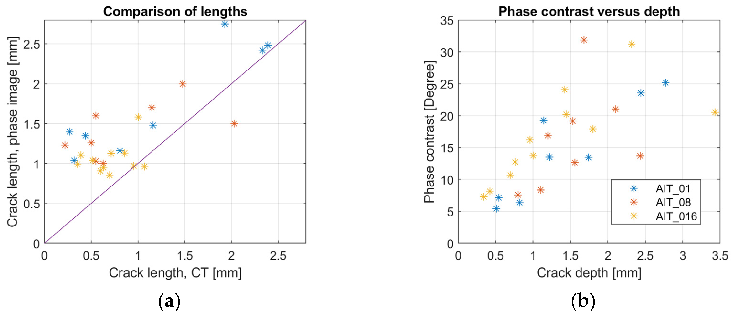
A comparison of both techniques was carried out for three samples, all of them manufactured by the Varestraint test machine. Figure 5a compares the crack lengths obtained from both techniques. Based on this figure, it can be observed that, in most cases, the crack length determined in the phase image is longer than it is determined in the CT results. This difference is probably caused by the software for evaluating the CT results, which maybe does not recognize the start of the cracks well enough, especially for shallow cracks.
In Figure 5b, the phase contrast for the cracks in the three inspected samples is depicted with dependency on the crack depth, which was determined from the CT measurements. It is well visible that the deeper the crack, the larger the phase contrast around it, as predicted through the finite element simulations. But, as the simulations also show, the phase contrast also depends on additional parameters, such as crack shape, inclination angle, and the orientation of the crack regarding the induced eddy currents.
6. Summary
Inductive thermography measurements were presented for Varestraint test samples, containing short cracks, with lengths up to 2.5 mm. The goal of these experiments was to show that very small cracks can be detected using inductive thermography. The length of the cracks can be determined by the distance of the hot spots in the phase image, occurring at the crack tips. On the other hand, the phase contrast around a crack depends not only on its length but is strongly affected by its depth. Additional CT measurements were carried out to determine the crack depths. Evaluation of the phase contrast versus the crack depth proves that the deeper the crack is, the larger its phase contrast. This investigation shows the main advantage of inductive thermography. Using this NDT technique, not only the defects can be localized but the phase image can also be used to characterize the cracks, as it gives information about the crack depth.
Funding
This project received funding from the Clean Sky 2 Joint Undertaking (JU) under grant agreement Nº. 101007699. The JU receives support from the European Union’s Horizon 2020 research and innovation program and the Clean Sky 2 JU members other than the Union.
Institutional Review Board Statement
Not applicable.
Informed Consent Statement
Not applicable.
Data Availability Statement
The data presented in this study are available on request from the corresponding author.
Acknowledgments
The CT measurements were carried out in GKN Areospace Engine Systems by Philipp Westphal, in Trollhättan in Sweden. The Varestraint test samples were manufactured in Lortek SCOOP in Ordizia in Spain.
Conflicts of Interest
The author declares no conflict of interest.
References
- Netzelmann, U.; Walle, G.; Lugin, S.; Ehlen, A.; Bessert, S.; Valeske, B. Induction thermography: Principle, applications and first steps towards standardisation. QIRT J. 2016, 13, 170–181. [Google Scholar] [CrossRef]
- DIN 54183:2018–02. Non-Destructive Testing-Thermographic Testing-Eddy-Current Excited Thermography. Available online: https://www.din.de (accessed on 10 January 2018).
- Srajbr, C. Induction excited thermography in industrial applications”, In Proceedings of the 19th World Conference on Non-Destructive Testing, Munich, Germany, 13–17 June 2016.
- Vrana, J.; Goldammer, M.; Baumann, J.; Rothenfusser, M.; Arnold, W. Mechanism and models for crack detection with induction thermography. AIP Conf Proc. 2008, 1706, 475–482. [Google Scholar] [CrossRef]
- Wilson, J.; Tian, G.Y.; Abidin, I.Z.; Yang, S.; Almond, D. Modelling and evaluation of eddy current stimulated thermography. Nondestruct. Test. Eval. 2010, 25, 205–218. [Google Scholar] [CrossRef]
- Oswald-Tranta, B. Detection and characterisation of short fatigue cracks by inductive thermography. QIRT J. 2021, 19, 239–260. [Google Scholar] [CrossRef]
- Oswald-Tranta, B.; Hackl, A.; Lopez de Uralde Olavera, P.; Gorostegui-Colinas, E.; Rosell, A. Calculating probability of detection of short surface cracks using inductive thermography. QIRT J. 2022. [Google Scholar] [CrossRef]
- Oswald-Tranta, B.; Lopez de Uralde Olavera, P.; Gorostegui-Colinas, E.; Westphal, P. Convolutional neural network for automated surface crack detection in inductive thermography. In Proceedings of the SPIE, Thermosense: Thermal Infrared Applications XLV, Orlando, FL, USA, 30 April–4 May 2023; Volume 12536. [Google Scholar]
Figure 1.
(a) Phase image of crack (depth = 0.5 mm, length = 1.5 mm), calculated via finite element simulations; the crack itself is marked as a red line; (b) simulated phase contrast values depending on crack length and depth.
Figure 1.
(a) Phase image of crack (depth = 0.5 mm, length = 1.5 mm), calculated via finite element simulations; the crack itself is marked as a red line; (b) simulated phase contrast values depending on crack length and depth.

Figure 2.
(a) Photo of the Varestraint test sample AIT_01, where short cracks in the welding region can be observed; (b) phase image of the same sample, obtained via inductive thermography measurement.
Figure 2.
(a) Photo of the Varestraint test sample AIT_01, where short cracks in the welding region can be observed; (b) phase image of the same sample, obtained via inductive thermography measurement.
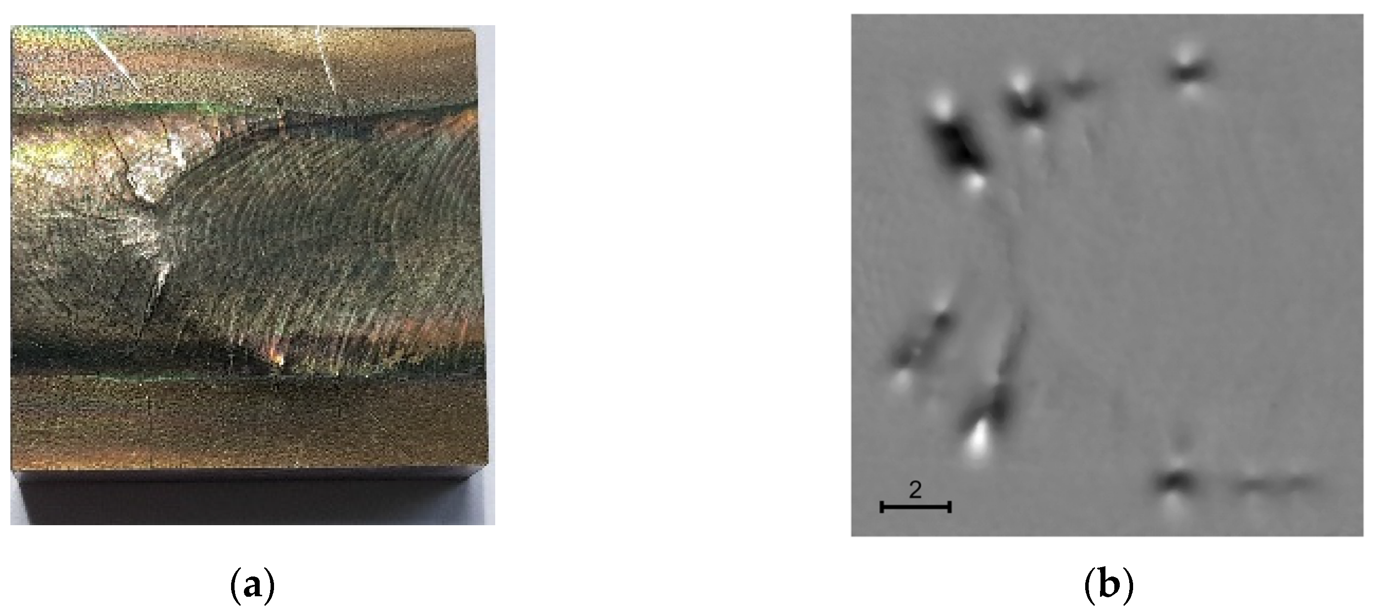
Figure 3.
CT results of the sample AIT_01, evaluated by a self-developed MATLAB routine in order to detect and to visualize the surface cracks.
Figure 3.
CT results of the sample AIT_01, evaluated by a self-developed MATLAB routine in order to detect and to visualize the surface cracks.
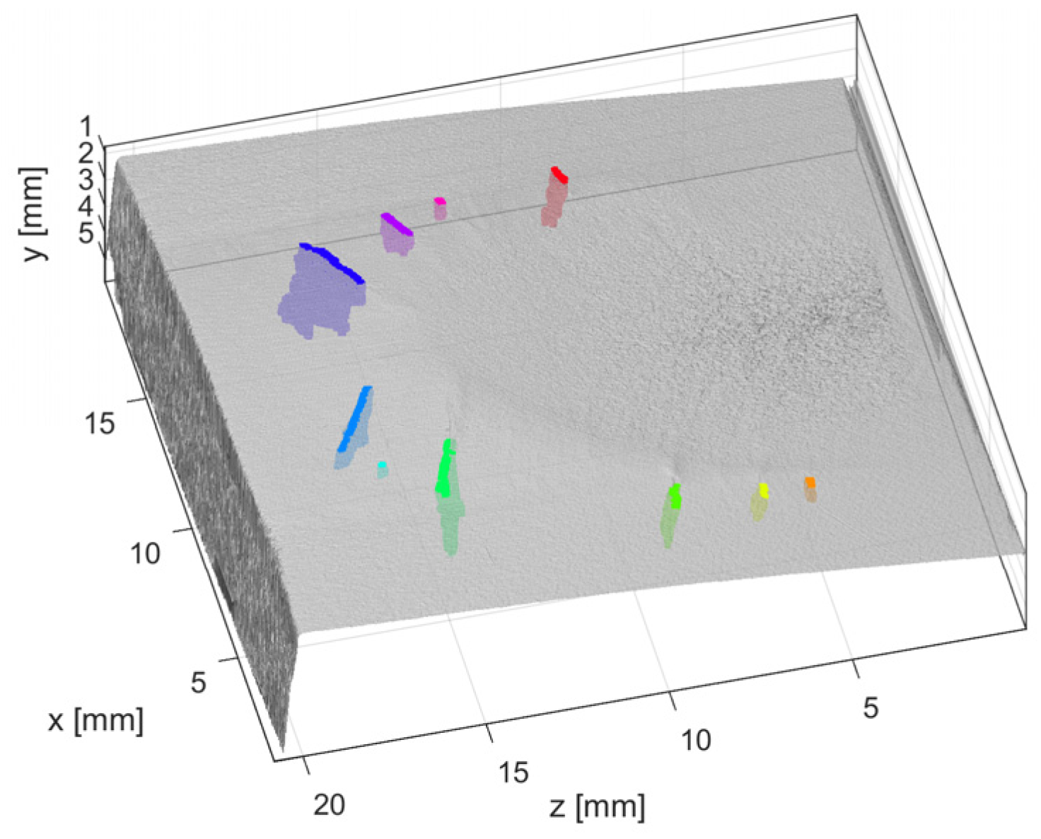
Figure 4.
(a) The phase image of sample AIT_01 with the 9 located cracks using a CNN; the phase contrast in degrees is written on each crack; (b) the defects localized in the CT results visualized additionally on the phase image. The crack lengths determined in the phase image are marked in both figures by red lines.
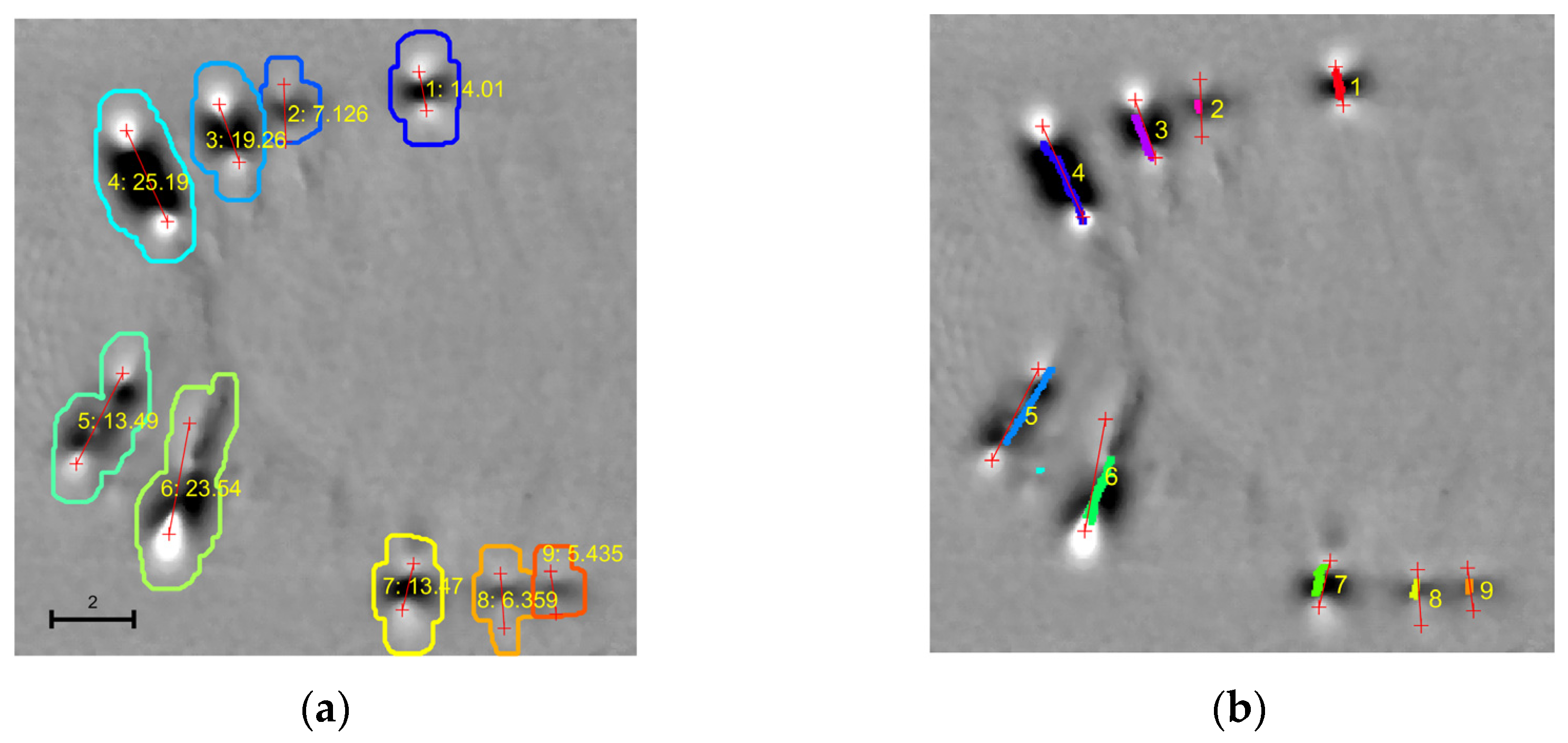
Figure 5.
(a) Comparison of crack lengths determined in the CT data and in the phase image; (b) phase contrast from the inductive thermography plotted against the crack depth, determined from the CT measurement. The data are plotted for the cracks localized in three samples.
Figure 5.
(a) Comparison of crack lengths determined in the CT data and in the phase image; (b) phase contrast from the inductive thermography plotted against the crack depth, determined from the CT measurement. The data are plotted for the cracks localized in three samples.
Disclaimer/Publisher’s Note: The statements, opinions and data contained in all publications are solely those of the individual author(s) and contributor(s) and not of MDPI and/or the editor(s). MDPI and/or the editor(s) disclaim responsibility for any injury to people or property resulting from any ideas, methods, instructions or products referred to in the content. |
© 2023 by the author. Licensee MDPI, Basel, Switzerland. This article is an open access article distributed under the terms and conditions of the Creative Commons Attribution (CC BY) license (https://creativecommons.org/licenses/by/4.0/).
Share and Cite
MDPI and ACS Style
Oswald-Tranta, B. Comparison of Inductive Thermography and Computer Tomography Results for Short Surface Cracks. Eng. Proc. 2023, 51, 36. https://doi.org/10.3390/engproc2023051036
AMA Style
Oswald-Tranta B. Comparison of Inductive Thermography and Computer Tomography Results for Short Surface Cracks. Engineering Proceedings. 2023; 51(1):36. https://doi.org/10.3390/engproc2023051036
Chicago/Turabian StyleOswald-Tranta, Beate. 2023. "Comparison of Inductive Thermography and Computer Tomography Results for Short Surface Cracks" Engineering Proceedings 51, no. 1: 36. https://doi.org/10.3390/engproc2023051036