
Numerical Analysis of Lid-Driven Cavity Flow Induced by Triangular Obstacles †


Department of Mechanical Engineering, National Institute of Technology Karnataka, Surathkal, Mangalore 575025, India
*
Author to whom correspondence should be addressed.
†
Presented at the International Conference on Recent Advances in Science and Engineering, Dubai, United Arab Emirates, 4–5 October 2023.
Eng. Proc. 2023, 59(1), 113; https://doi.org/10.3390/engproc2023059113
Published: 24 December 2023
(This article belongs to the Proceedings of Eng. Proc., 2023, RAiSE-2023)
Abstract
:This research work presents a study on the flow behaviour in the lid-driven cavity (LDC) flows with triangular blocks using computational fluid dynamics techniques. The LDC flow is a widely studied problem that remains a standard for viscous incompressible fluid flows, with a range of parameters, including the Reynolds number, being explored. The finite volume method was used to discretize the domain, and simulations were computed using ANSYS FLUENT 2021 R1. The fluid flow started when the top wall is moved in the +X direction, whereas the other three walls are kept stationary. A grid independence test was performed to determine the optimum grid size and to obtain a grid-independent solution. Quantitative elements of the 2D flows in lid-driven cavities were explored for Reynolds numbers ranging from 1000 to 8000, and the results were validated against the existing literature. The consequence of different values of the Reynolds number (Re) were analyzed and examined through vorticity, streamline patterns, and kinetic energy contours. The velocity profile at the centerline was enhanced, and the vortex number and size increased with an increase in Re. The behaviour of the isolines of the vortices and the kinetic energy contours was also analyzed. The kinetic energy contours show that the high velocity of the fluid particles close to the upper wall is a significant factor affecting the maximum kinetic energy values. As the Reynolds number increased, the kinetic energy gradually increased at the boundary. This suggests that the Re considerably affects the energy values. Overall, this study provides valuable insights into the flow behaviour of lid-driven cavities and the effects of obstacles on flow patterns, contributing to the existing literature and being useful for researchers and engineers working in the field of fluid dynamics.
1. Introduction
Computational Fluid Dynamics (CFD) is a process that involves the mathematical modelling of physical phenomena related to fluid flow and solving it numerically using computational resources [1,2,3,4,5]. CFD assumes a significant role in both experimental and theoretical fields. Specifically, CFD uses data structures and numerical methods to analyze and solve fluid flow problems. Lid-driven cavity flow is a common problem that has been studied comprehensively and has not lost its position as a standard problem for viscous incompressible fluid flows. In recent years, the vast application of CFD in the fields of electronics, crystal growth, and food processing has led to an increase in the number of studies on LDC, along with the diverse parameters involved, such as the Reynolds number [6,7,8,9]. The LDC problem is a simple 2D problem involving a square area with one wall, preferably the top wall, moving with a familiar velocity, and the remaining three walls are immobile. This obstacle problem is considered a straightforward model for investigating the fluid flow observed in processing industries. Furthermore, separations and obstacles of various forms are used inside a closed space to achieve effective fluid behaviour.
2. Literature Review and Objectives
Ghia et al. [10] employed the multigrid method to solve the Navier—Stokes equation and obtained solutions for different Reynolds numbers. This paper obtained high—Re flow fine—mesh solutions with high efficiency using the coupled strongly implicit and multigrid methods. The authors observed that the finest mesh size used in the grid sequence is quite a significant parameter. For Reynolds numbers ranging from 100–7500, Lin et al. [11] used the multi-relaxation time LBM to compute properties in an LDC for aspect ratios of 1, 1.5, and 4. Azwadi et al. [12] used the Adams—Bashforth scheme to numerically study an LDC with four moving walls. They observed that an increase in the Reynolds number was accompanied by an increase in the proximity of the vortices to the diagonal joining the cavity edge. It was seen that the structure in the domain is predominantly influenced by the Reynolds number. Gokhale and Fernandes [13] simulated laminar flow for various values of Reynolds numbers ranging from 10 to 2000 using the LBM method and observed that the higher the Reynolds number, the greater the vortex shift to the centre from the right side. Using the LBM method, Safdari and Kim [14] employed this approach in a three-dimensional cubic cavity consisting of solid particles. When the breadth of the Reynolds numbers was taken, it was seen that the particles managed to shift towards the boundary walls. In another work, Zhuo and Zhong [15] found that at a Reynolds number of 720, Hopf bifurcation of flows was observed after investigating four complex LDC domains using the LBM-MRT for an extensive range of Reynolds numbers.
Perumal and Dass [16] documented the numerical outcomes of the LDC domain using the LBM equation. The effects of different Re and aspect ratios on the flow characteristics were studied. The appearance of secondary and tertiary vortices was observed at a higher Reynolds number and their shapes changed with the increasing aspect ratio. Endang et al. [17] implemented a finite—difference approach with a pressure correction method on a double—sided lid-driven cavity for Reynolds numbers ranging from 100–10,000. Souayeh [18] introduced circular and spherical obstacles into 2D and 3D LDCs and studied their unsteady states introduced by them. The FVM, along with the full multigrid technique, is used to solve this problem. Due to Hopf bifurcation, the flow regime oscillates above a critical Reynolds number value. Hence, the grid size variation and model sizes significantly influenced the critical Re.
However, the literature does not predict the unsteady states inside a lid—driven cavity when a central triangular block is used as an obstacle. This paper provides a comprehensive review of studies on the lid—driven cavity flows and their findings, followed by a computational analysis of the steady—state, 2D incompressible flow in an LDC square enclosure with several triangular blocks of blockage of 10%.The manuscript is organized as follows. The 3rd section presents the physical model and expression of the computed problem. Numerical methodology and the grid sensitivity analysis are presented in this section. The LDC results for a range of Re values, and concluding remarks are made in the final sections, respectively.
3. Methodology
3.1. Physical Model and Mathematical Formulation
The methods should be described with sufficient details to allow others to a square—sided LDC with sides H = L consisting of a triangular block of side b = 0.1H, as shown in Figure 1.The velocity of the topmost wall is set to unity in the positive direction. The Reynolds number is a crucial parameter that determines the flow properties, and it establishes laminar or turbulent flow patterns. From the description of the Reynolds number, Re = uoh/ν, where u0 is the involved velocity at the upper wall, h = L is the length, and ν represents the kinematic viscosity of the fluid. The distance between the centroids of the triangle was set to 0.5L when multiple obstacles were used in Figure 2. Simulations were conducted for Reynolds numbers varying from 1000 to 8000, as the flow contours for laminar and turbulent cases must be analyzed. The governing equations in the dimensionless form are expressed as follows:
Continuity equation
Momentum equation
The dimensionless form of the coordinate space is represented using xi and the velocity components by ui, the hydrodynamic pressure using p, and time using t. According to the geometric model, the pressure and velocity boundary conditions are enumerated as follows: moving wall: u = 1, v = 0, that is at y = 1 and u = 0, v = 0 on the stationary walls that is at x = 0, x = 1, and y = 0.
3.2. Numerical Methodology and Grid Sensitivity Analysis
The FVM is implemented to split the domain into a set of linear equations and then solved using numerical methods, particularly the Gauss—Seidel point—by—point iterative method. Because the problem involves a steady—state simulation where the solution remains relatively constant over time, an iterative method like the Gauss—Seidel method is more effective and preferred over direct solvers in such a scenario.These numerical computations were performed using the student version of ANSYS FLUENT 2021 R1. The finite volume method was used because it inherently conserves quantities like mass, momentum, and energy within the control volumes. This makes it particularly well-suited for problems involving conservation laws, such as fluid dynamics. In addition, because the ANSYS FLUENT software 2021R1 uses FVM as its default method for solving fluid problems, it was used. Unstructured mesh elements with consistent grid spacing were developed. Toobtain a faster convergence and stabilizationof the case, an implicit under—relaxation pseudo—transient was enabled. The steady—state simulations were assumed to be converged if the residuals fell below 10−6 such that
Here Φ represents a generic variable that denotes the pressure, U, and V velocities, m being the iteration level, and the X and Y space coordinates are indicated by the subscripts (i, j).Grid sensitivity analysis was performed for Re = 1000 to ensure a grid—independent solution. Three different non—uniform grids, namely 642, 1282, and 2562, wereutilized to simulate the present problem. The corresponding umin and vmin values are enumerated in Table 1.
It can be noticed that the percentage error in the solution decreases to as low as 0.44% when the mesh size increases. A non-uniform grid of 256 × 256 provides reasonably accurate results, and the computation time needed is also less as shown in Table 2. Hence, a 2562 grid size with 65,780 nodes and 65,233 elements was adequate to determine the necessary dynamics. Therefore, this mesh structure was employed to perform all the subsequent calculations.
4. Results and Discussion
The numerical results demonstrated regarding streamlines, vorticity, and kinetic energy for specific Reynolds numbers are shown in Figure 3, Figure 4 and Figure 5, respectively. For more accurate results, various grid sizes of 642, 1282, and 2562 were used for each Reynolds number (1000, 5000, and 8000, respectively). A personal computer with an Intel Core i5-8300H processor and a CPU that is rated at a clock speed of 2.3 GHz was used to conduct the numerical simulations. The model was validated by comparing the velocity extrema along the centerlines generated by Souayeh [18], Cazemier et al. [19], and Gouillart and Thiffeault [20] for Re = 1000. These results are enumerated in Table 3, and it is seen that these results show reasonable proximity to the existing literature.
In Figure 3, we can observe four vortices: one primary vortex at the centre, a couple of secondary vortices at the two bottom corners, and a tertiary small vortex at the top—left of the cavity for Re = 5000 and 8000. With a gradual increase in the Reynolds number from 1000 to 8000, we see that the minimum and maximum rates of ψ increase. The isolines of vortices, that is, the vorticity contours, are plotted in Figure 4. The kinetic energy is expressed as Ec = 0.5*(u2 + v2), and its contours are shown in Figure 5. The high speed of the fluid particles near the top wall contributes to the maximum kinetic energy values. At the moving wall, the kinetic energy slowly increases with the increasing Reynolds number. This indicates that the energy values are considerably influenced by the Reynolds numbers, especially in the high—speed region surrounding the moving wall.
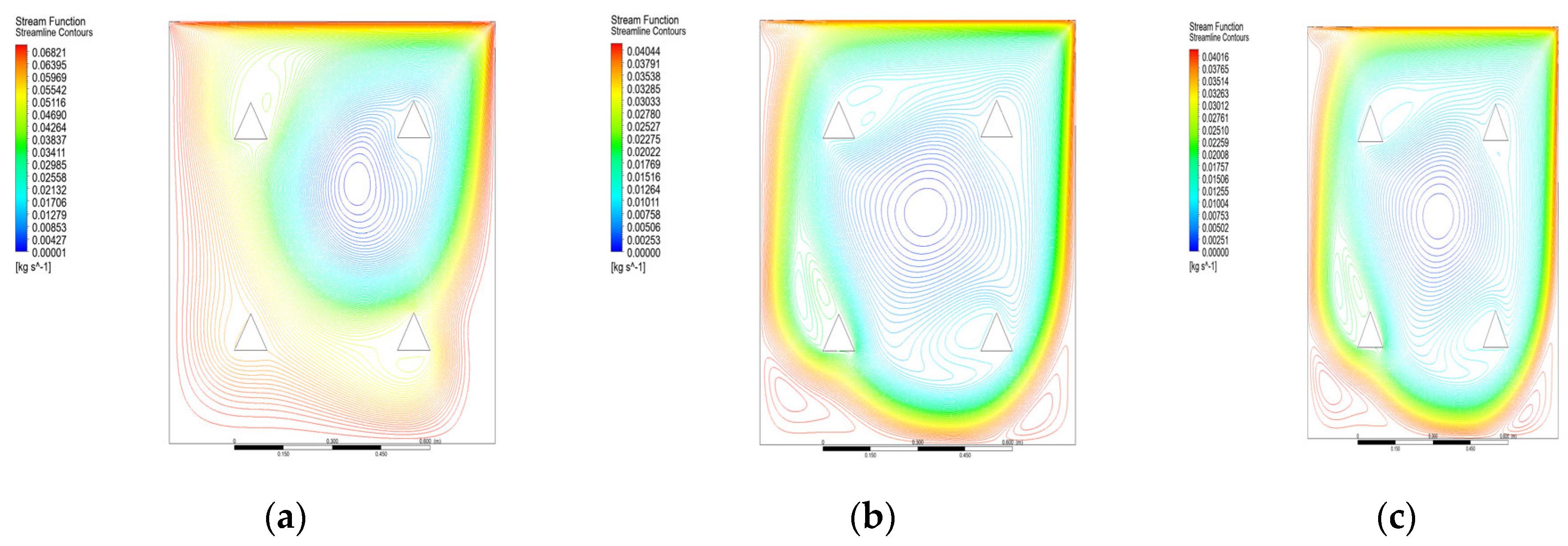
Figure 6 and Figure 7 show the deviation of the extreme ψ rates and extreme vorticity components as Re. Here, we see that Ψmax increases until a particular value of the Reynolds number and then decreases, whereas the Ψmin value slightly decreases and then increases. A similar trend was seen in the variation in the extreme vorticity components. The current study considers various triangular obstacles in a lid-driven cavity. Figure 8 and Figure 9 illustrate the streamlined patterns at various Reynolds numbers with two and four triangular impediments in the domain, respectively. The Re, and the number, size, and vortex location within the cavity also vary.
With an increase in the Reynolds number, the strength and size of the corner vortices increased, whereas the distance between the cavity center and the primary vortex decreases. The formation of secondary vortices can be seen around the obstacle, and the flow structures inside the cavity tend to become more complicated. The results, including streamlines, vorticity, and kinetic energy contours, were compared with benchmark solutions. Streamlines reveal primary and secondary vortices, with stream function values increasing and then decreasing as the Reynolds numbers increased. The extreme vorticity and stream function values exhibit similar trends. The velocity values along the centerlines closely match with previous research. Additionally, the study examined the effect of triangular obstacles on flow patterns and found that the number, size, and location of vortices change with varying Reynolds numbers.
5. Conclusions
In the present study, triangular obstacles were introduced in the LDC domain, and the flow induced by triangular obstacles was investigated for the 2D configuration. As Re increased, the velocity profiles at the centerline were enhanced, causing the growth of the secondary vortex located at the corners of the bottom. The study concluded that triangular obstacles in an LDC induce complex flow patterns that vary with the Reynolds number. A reasonable concurrence was found when comparisons were conducted with prior literature, particularly those that had existing data related to the lid—driven cavity flows. The illustrated representation results are then presented and examined. Finally, the number and size of the vortices that emerge in the cavity center increase with an increase in the Reynolds number. The future scope of research can explore lid—driven cavities containing various obstacles, with multiphase flows that can include the modeling of bubbles, droplets, or solid particles within the cavity. It can have an LDC flow subject to the study of the heat transfer effects. A simulation of Non-newtonian fluids in a lid—driven cavity was performed. The interaction of chemical reactants or electromagnetic fields in a domain can also be investigated.
Author Contributions
Conceptualization and methodology: D.A.P. and S.N.H.; software, validation, investigation, formal analysis, visualization, writing—original draft preparation, resources, data curation: N.L.B.; Supervision, project administration, writing—review and editing: D.A.P. All authors have read and agreed to the published version of the manuscript.
Funding
This research received no external funding.
Institutional Review Board Statement
Not applicable.
Informed Consent Statement
Not applicable.
Data Availability Statement
All data are included in the manuscript.
Acknowledgments
Authors thank Department of Mechanical Engineeing, NIT Karnataka, Surathkal, for providing the computational facilities.
Conflicts of Interest
The authors declare no conflict of interest.
References
- Bhopalam, S.R.; Perumal, D.A.; Yadav, A.K. Computational appraisal of fluid flow behavior in two-sided oscillating lid-driven cavities. Int. J. Mech. Sci. 2021, 196, 1–15. [Google Scholar] [CrossRef]
- Bhopalam, S.R.; Perumal, D.A. Numerical analysis of fluid flows in L-Shaped cavities using Lattice Boltzmann method. Appl. Eng. Sci. 2020, 3, 1–14. [Google Scholar]
- Rajan, I.; Perumal, D.A. Flow Dynamics of Lid-Driven Cavities with obstacles of various shapes and configurations using the Lattice Boltzmann Method. J. Therm. Eng. 2021, 7, 83–102. [Google Scholar] [CrossRef]
- Perumal, D.A. Lattice Boltzmann Computation of Multiple Solutions in a Double-Sided Square and Rectangular Cavity Flows. Therm. Sci. Eng. Prog. 2018, 6, 48–56. [Google Scholar] [CrossRef]
- Perumal, D.A.; Dass, A.K. Multiplicity of steady solutions in two-dimensional lid driven cavity flows by Lattice Boltzmann method. Comput. Math. Appl. 2011, 61, 3711–3721. [Google Scholar] [CrossRef]
- Xie, B.; Xiao, F. A multi-moment constrained finite volume method on arbitrary unstructured grids for incompressible flows. J. Comput. Phys. 2016, 327, 747–778. [Google Scholar] [CrossRef]
- Zamzamian, K.; Hashemi, M.Y. A novel meshless method for incompressible flow calculations. Eng. Anal. Bound. Elem. 2015, 56, 106–118. [Google Scholar] [CrossRef]
- Jiang, Y.; Mei, L.; Wei, H. A finite element variational multiscale method for incompressible flow. Appl. Math. Comput. 2015, 266, 374–384. [Google Scholar] [CrossRef]
- Perumal, D.A.; Dass, A.K. Application of Lattice Boltzmann method for incompressible viscous flows. Appl. Math. Model. 2011, 37, 4075–4092. [Google Scholar] [CrossRef]
- Ghia, U.; Ghia, K.N.; Shin, C.T. High-resolutions for incompressible flow using the Navier–Stokes equations and a multigrid method. J. Comput. Phys. 1982, 48, 387–411. [Google Scholar] [CrossRef]
- Lin, L.S.; Chen, Y.C.; Lin, C.A. Multi relaxation time lattice Boltzmann simulations of deep lid driven cavity flows at different aspect ratios. Comput. Fluids 2011, 45, 233–240. [Google Scholar] [CrossRef]
- Azwadi, C.S.N.; Rajab, A.; Sofianuddin, A. Four-sided lid driven cavity flow using time splitting method of Adams-Bashforth scheme. Int. J. Automot. Mech. Eng. 2014, 9, 1501–1510. [Google Scholar] [CrossRef]
- Gokhale, F. Lattice Boltzmann simulation of fluid flow in a lid driven cavity. Int. J. Mech. Eng. Robot. 2014, 2, 1–5. [Google Scholar]
- Safdari, A.; Kim, K.C. Lattice Boltzmann simulation of solid particles behavior in a three-dimensional lid-driven cavity flow. Comput. Math. Appl. 2014, 68, 606–621. [Google Scholar] [CrossRef]
- Zhuo, C.; Zhong, C.; Guo, X.; Cao, J. Numerical investigation of four-lid-driven cavity flow bifurcation using the multiple-relaxation-time lattice Boltzmann method. Comput. Fluids 2015, 110, 136–151. [Google Scholar] [CrossRef]
- Perumal, D.A.; Dass, A.K. A review on the development of Lattice Boltzmann computation of Macro fluid flows and Heat Transfer. Alex. Engg J. 2015, 54, 955–971. [Google Scholar] [CrossRef]
- Endang, M.; Eko, P.B.; Yuana, K.A.; Kamal, S. Deendalinto, Simulation of lid-driven cavity with top and bottom moving boundary conditions using implicit finite difference method and staggered grid. AIP Conf. Proc. 2018, 2021, 020002. [Google Scholar]
- Souayeh, B.; Alam, M.W.; Hammami, F.; Hdhiri, N.; Yasin, E. Predicting the unsteady states of 2D and 3D lid-driven cavities induced by a centrally located circle and sphere. Fluid Dyn. Res. 2020, 52, 025507. [Google Scholar] [CrossRef]
- Cazemier, W.; Verstappen, C.P.; Veldman, E.P. Proper orthogonal decomposition and low dimensional model for driven cavity flow. Phys. Fluids 1998, 10, 1685–1699. [Google Scholar] [CrossRef]
- Gouillart, T. Topological mixing of viscous fluids. In Proceedings of the Condensed Matter Seminar, Edinburgh, UK, 5 June 2006. [Google Scholar]
Figure 1.
The geometry of a lid-driven cavity having (a) one, (b) two, and (c) four triangular blocks.
Figure 1.
The geometry of a lid-driven cavity having (a) one, (b) two, and (c) four triangular blocks.
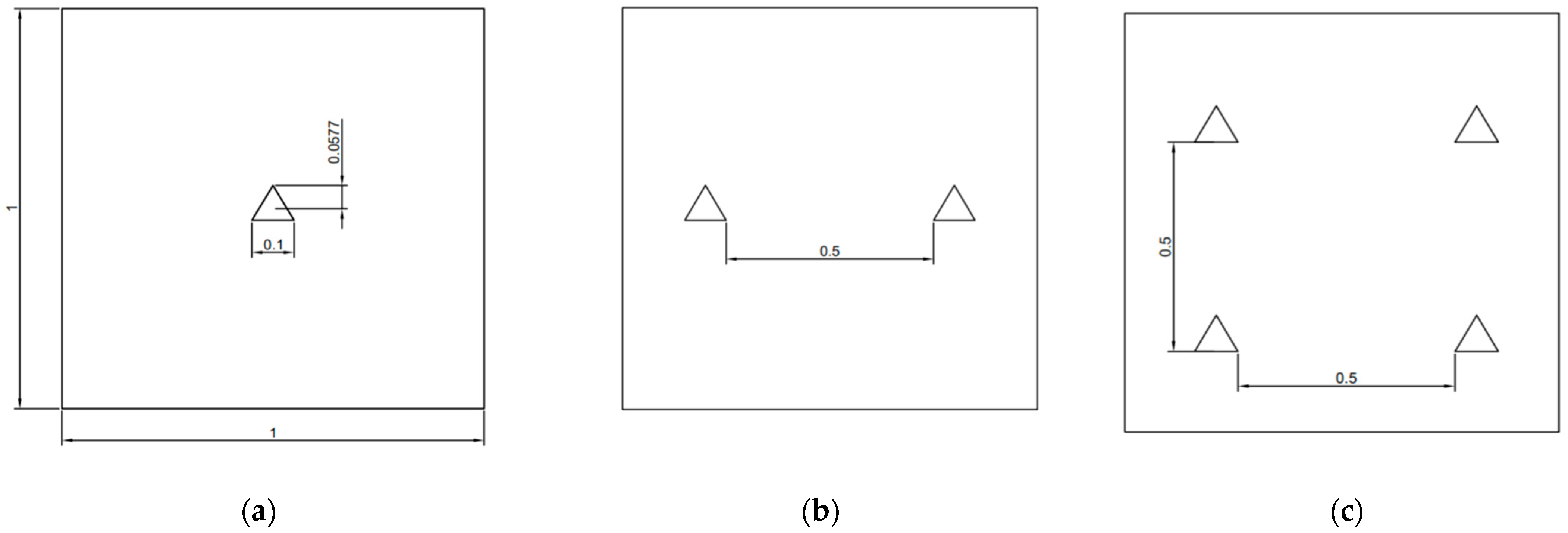
Figure 2.
The meshing of the lid-driven cavity has (a) one, (b) two, and (c) four triangular blocks.
Figure 2.
The meshing of the lid-driven cavity has (a) one, (b) two, and (c) four triangular blocks.
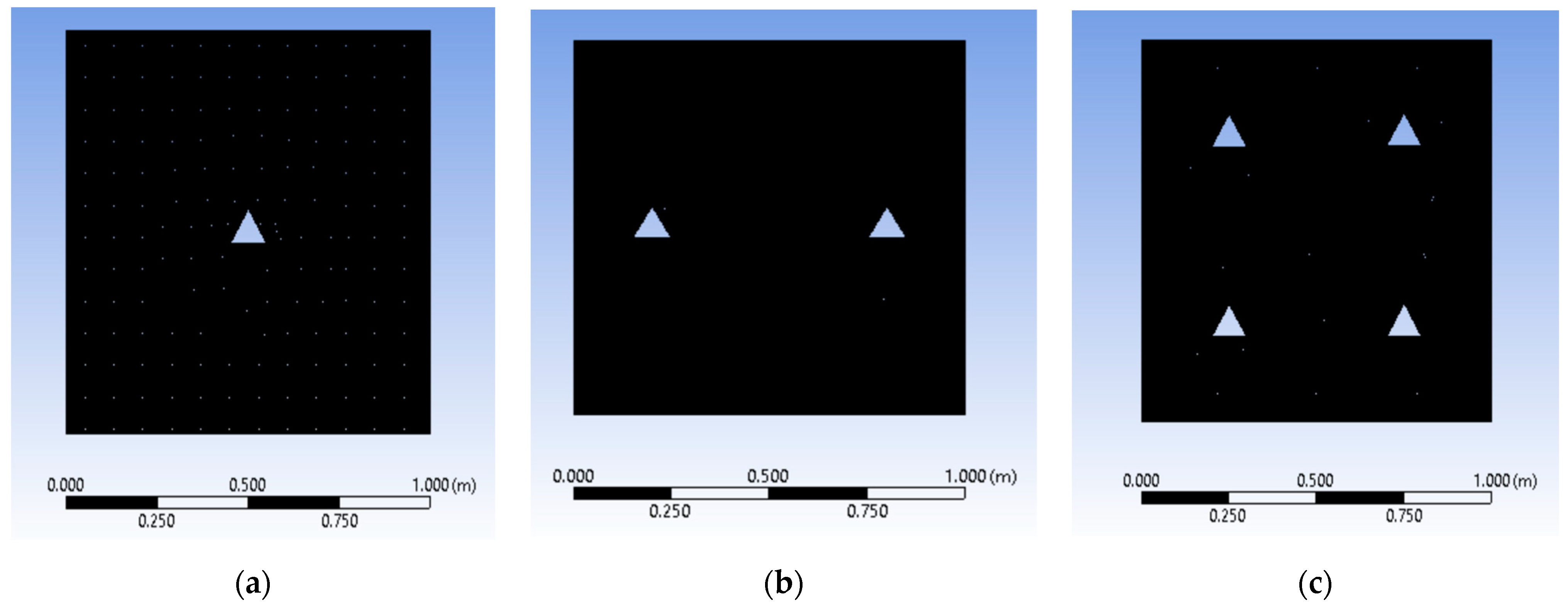
Figure 3.
Streamlines for Reynolds numbers of (a) 1000, (b) 5000, and (c) 8000 for the grid size of 2562.
Figure 3.
Streamlines for Reynolds numbers of (a) 1000, (b) 5000, and (c) 8000 for the grid size of 2562.
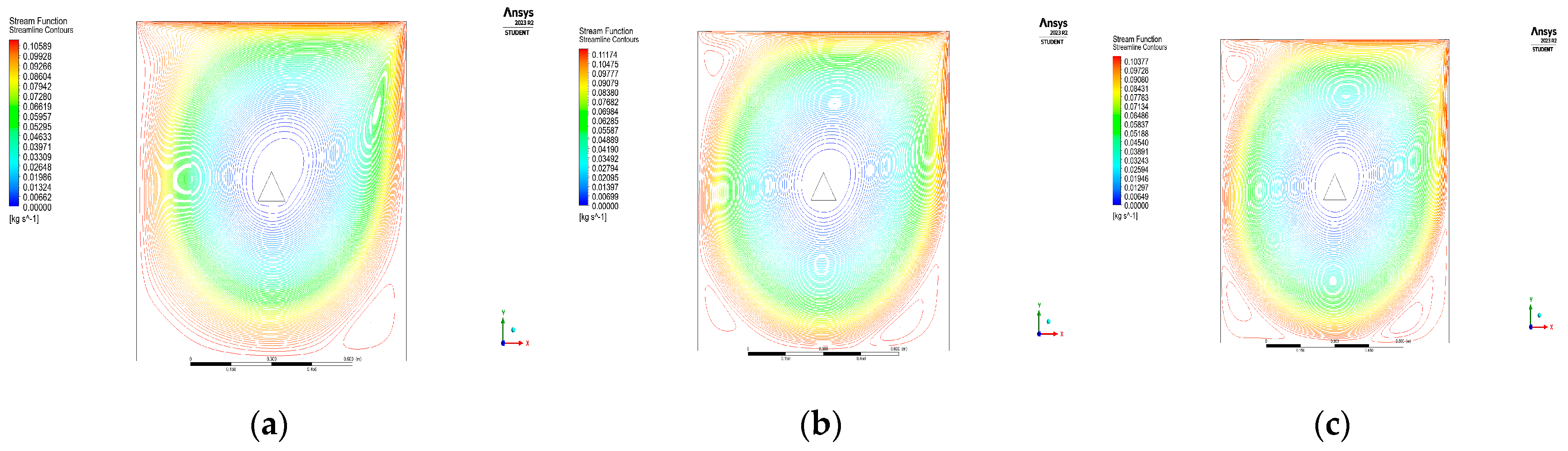
Figure 4.
Vorticity contours for Reynolds numbers of (a) 1000, (b) 5000, and (c) 8000 for the grid size of 2562.
Figure 4.
Vorticity contours for Reynolds numbers of (a) 1000, (b) 5000, and (c) 8000 for the grid size of 2562.
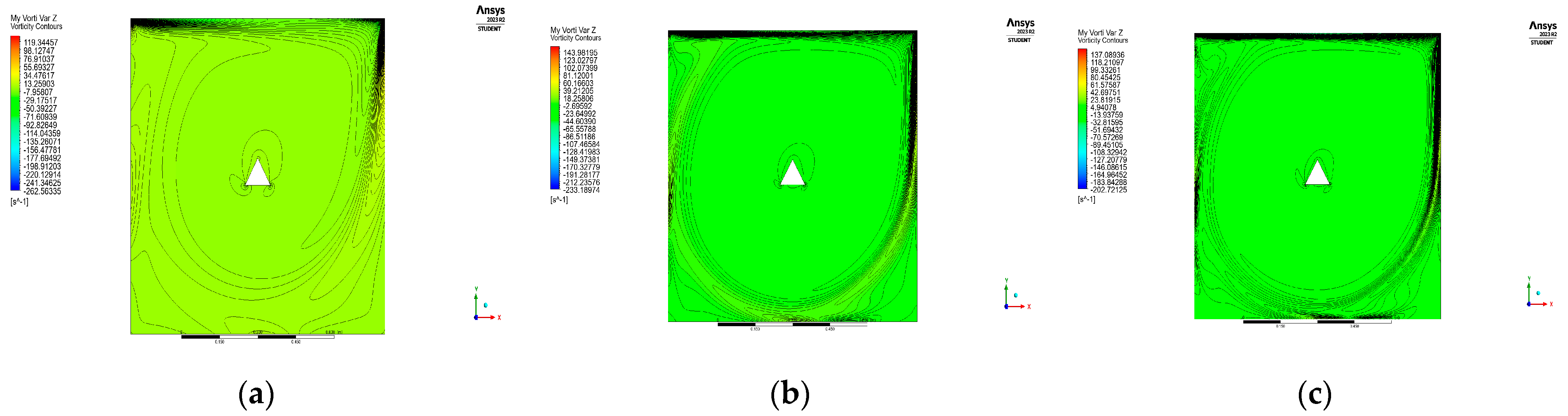
Figure 5.
Kinetic energy contours for Reynolds numbers of (a) 1000, (b) 5000, and (c) 8000 for the grid size of 2562.
Figure 5.
Kinetic energy contours for Reynolds numbers of (a) 1000, (b) 5000, and (c) 8000 for the grid size of 2562.
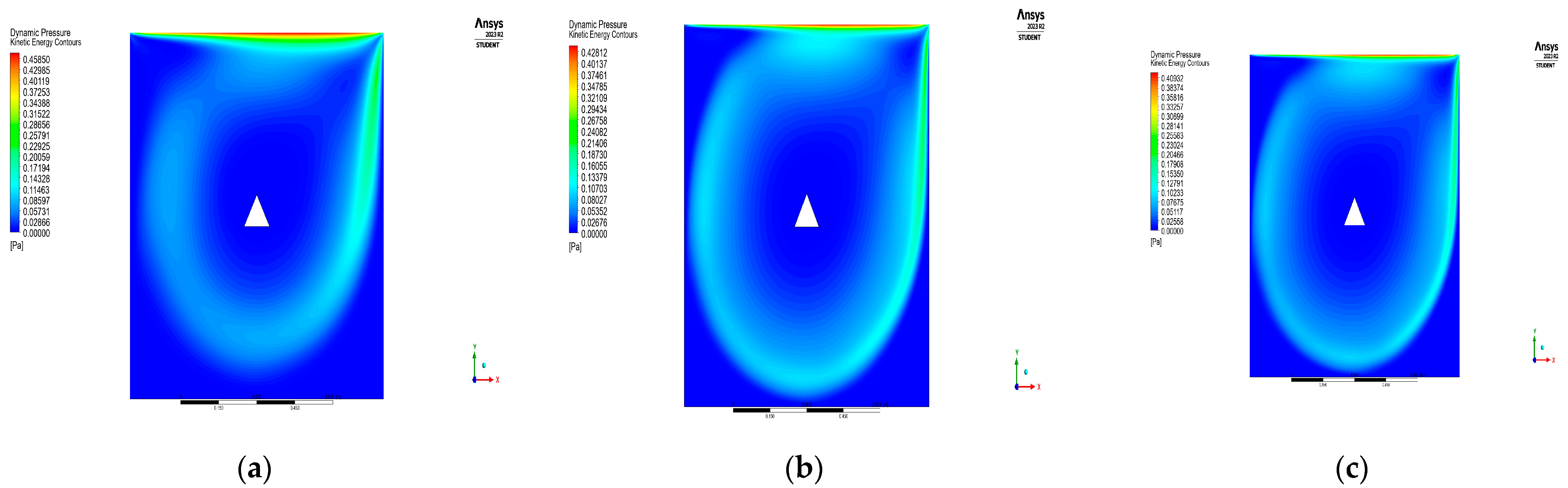
Figure 6.
(a) Maximum and (b) Minimum component of stream function vs. Reynolds number for various grid sizes.
Figure 6.
(a) Maximum and (b) Minimum component of stream function vs. Reynolds number for various grid sizes.
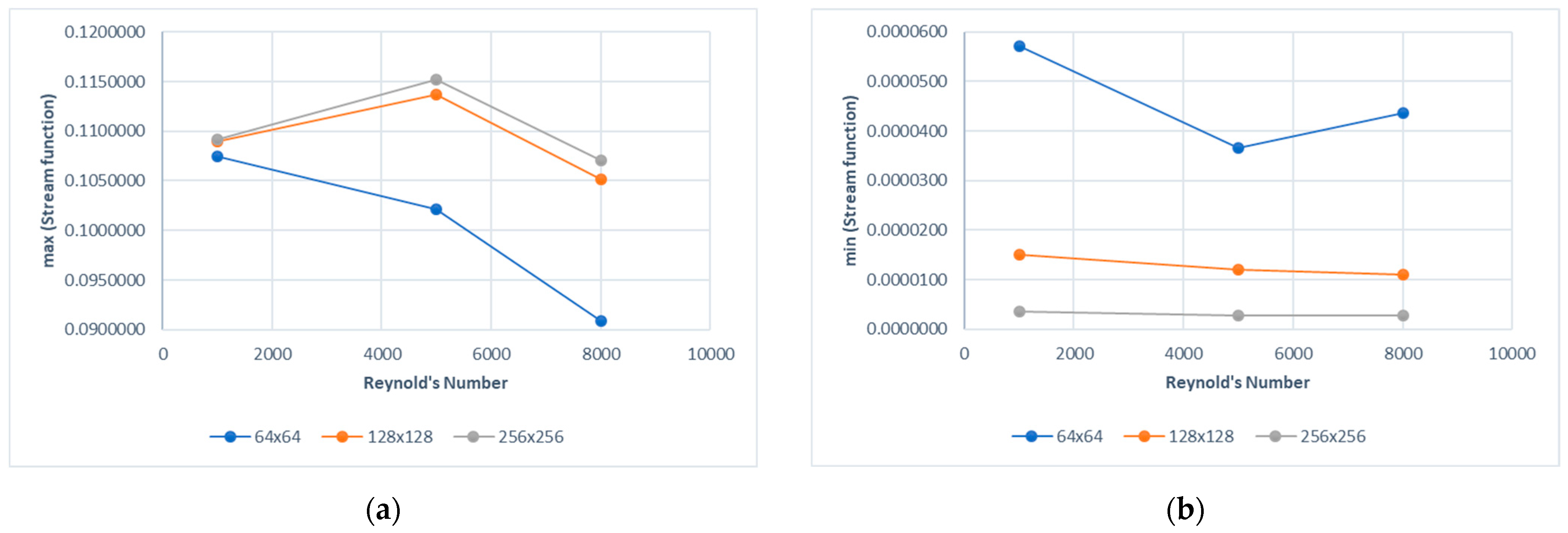
Figure 7.
(a) Maximum and (b) Minimum component of vorticity vs. Reynolds number for various grid sizes.
Figure 7.
(a) Maximum and (b) Minimum component of vorticity vs. Reynolds number for various grid sizes.
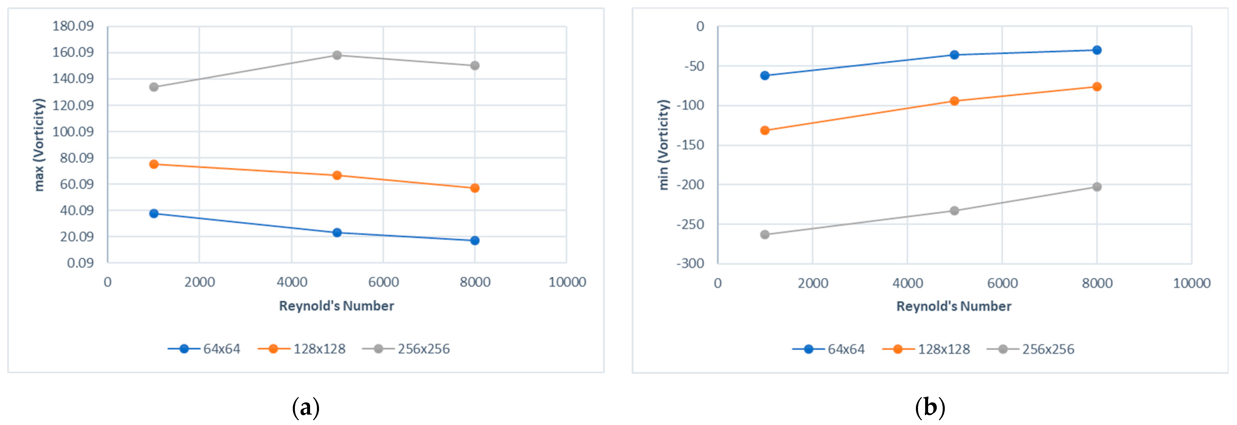
Figure 8.
Streamlines for Reynolds numbers of (a) 1000, (b) 5000, and (c) 8000 for the grid size of 2562 for a cavity with two obstacles.
Figure 8.
Streamlines for Reynolds numbers of (a) 1000, (b) 5000, and (c) 8000 for the grid size of 2562 for a cavity with two obstacles.
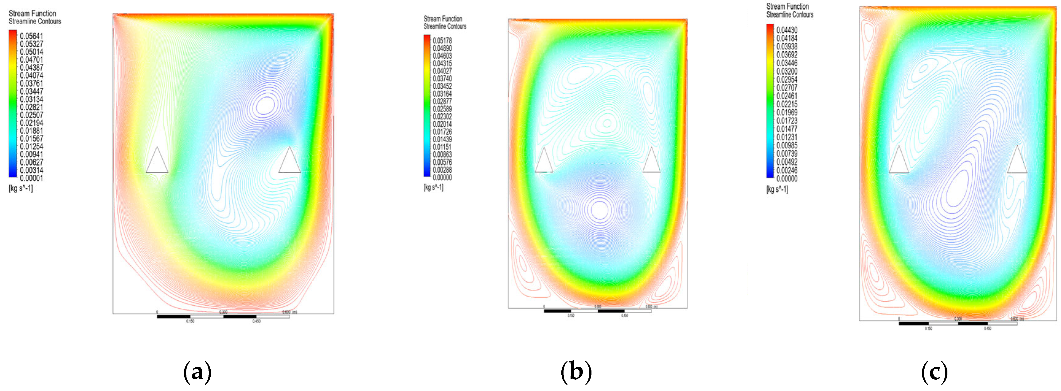
Figure 9.
Streamlines for Reynolds numbers of (a) 1000, (b) 5000, and (c) 8000 for the grid size of 2562 for a cavity with four obstacles.
Figure 9.
Streamlines for Reynolds numbers of (a) 1000, (b) 5000, and (c) 8000 for the grid size of 2562 for a cavity with four obstacles.

Table 1.
Grid independencetest for Re = 1000.
| Grid Size for Re = 1000 | umin | vmin |
|---|---|---|
| 64 × 64 | −0.374630 | −0.635462 |
| 128 × 128 | −0.382873 (2.2%) | −0.668224 (5.155%) |
Table 2.
Stream function extrema values for Re = 1000 through the centerlines of the cavity for the grid size of 2562.
Table 2.
Stream function extrema values for Re = 1000 through the centerlines of the cavity for the grid size of 2562.
| Ψmin | xmin | ymin | Ψmax | xmax | ymax |
|---|---|---|---|---|---|
| 0.000004 | 0.562781 | 0.593031 | 0.109204 | 0.87188 | 0.113281 |
Table 3.
Maximum and minimum values of u through the centerlines of the cavity for Re = 1000 corresponding to the grid size 2562.
Table 3.
Maximum and minimum values of u through the centerlines of the cavity for Re = 1000 corresponding to the grid size 2562.
| umin | ymin | vmax | xmax | vmin | xmin | |
|---|---|---|---|---|---|---|
| Present Work | −0.384500 | 0.167969 | 0.377915 | 0.152318 | −0.674865 | 0.972656 |
| Souyayeh et al. [18] | −0.388300 | 0.169800 | 0.376800 | 0.156400 | 0.5270000 | 0.908800 |
| Gouillart and Thiffeault [20] | −0.382800 | 0.171900 | 0.370900 | 0.156300 | −0.515500 | 0.906300 |
| Cazemier et al. [19] | −0.386900 | 0.180000 | 0.375600 | 0.150000 | −0.526300 | 0.910000 |
Disclaimer/Publisher’s Note: The statements, opinions and data contained in all publications are solely those of the individual author(s) and contributor(s) and not of MDPI and/or the editor(s). MDPI and/or the editor(s) disclaim responsibility for any injury to people or property resulting from any ideas, methods, instructions or products referred to in the content. |
© 2023 by the authors. Licensee MDPI, Basel, Switzerland. This article is an open access article distributed under the terms and conditions of the Creative Commons Attribution (CC BY) license (https://creativecommons.org/licenses/by/4.0/).
Share and Cite
MDPI and ACS Style
Hegde, S.N.; Bendre, N.L.; Perumal, D.A. Numerical Analysis of Lid-Driven Cavity Flow Induced by Triangular Obstacles. Eng. Proc. 2023, 59, 113. https://doi.org/10.3390/engproc2023059113
AMA Style
Hegde SN, Bendre NL, Perumal DA. Numerical Analysis of Lid-Driven Cavity Flow Induced by Triangular Obstacles. Engineering Proceedings. 2023; 59(1):113. https://doi.org/10.3390/engproc2023059113
Chicago/Turabian StyleHegde, Sumanth N., Nihal L. Bendre, and D. Arumuga Perumal. 2023. "Numerical Analysis of Lid-Driven Cavity Flow Induced by Triangular Obstacles" Engineering Proceedings 59, no. 1: 113. https://doi.org/10.3390/engproc2023059113