


The Dynamic Properties of Sand under Torsion: A Literature Review

Structural and Geotechnical Engineering Department, Faculty of Architecture, Civil and Transport Sciences, Széchenyi István University, 9026 Gyor, Hungary
*
Author to whom correspondence should be addressed.
Geotechnics 2023, 3(2), 480-514; https://doi.org/10.3390/geotechnics3020027
Submission received: 15 May 2023
/
Revised: 7 June 2023
/
Accepted: 8 June 2023
/
Published: 11 June 2023
(This article belongs to the Special Issue Recent Advances in Geotechnical Engineering)
Abstract
:Resonant column (RC) and the torsional simple shear (TOSS) tests have shown proven competency in acquiring precise and repeatable measurements regarding the shear modulus and damping ratio of soil. For most dynamic geotechnical problems, the shear modulus represents the stiffness of the soil, while the damping ratio describes energy dissipation. Many studies in the last few decades focused on developing the relevant equipment and investigating the effect of different soil properties on the dynamic behavior of soil. Researchers have introduced correlations to approximate this behavior without conducting dynamic torsional testing. Soil models (e.g., Ramberg-Osgood and Hardin-Drnevich) can simulate shear stress-strain curves after finding the curve-fitting parameters. Due to the complexity of dynamic behavior and its dependency on various factors in soils, the RO and HD equations help model the behavior more simply. This paper presents a literature review and evaluation of the studies, correlations, soil models, and parameters affecting the dynamic behavior of dry sand under torsion.
1. Introduction
In engineering practice, static loading produces most of the actions considered in geotechnical design. However, as structures have evolved and material costs have significantly increased, a more advanced approach has required engineers to consider structures subjected to dynamic loading. Designers can no longer assume quasi-static behavior for dynamic conditions and apply overly generous safety factors. Newer designs demand a more detailed assessment of material dynamic properties and the interactions between soil, foundation, and structure. Newer designs require a better understanding of the dynamic behavior of both soil and structure.
The response of structures to dynamic loading is directly related to the response of soil beneath and around it. Therefore, many researchers in the past few decades focused on studying the behavior of soils subjected to dynamic loading. When earthquake waves propagate through the soil, they often pass upward through layers that usually become less stiff (lower modulus) as they approach the surface. The reduction is generally due to decreasing confining stresses in the soil, directly reducing its stiffness and strength. A consequence of the stiffness reduction is that the propagating waves refract to a more vertical path. The propagating waves travel vertically at many building locations, with most of their energy carried by shear waves. The surface ground motion consists of two horizontal (N-S and E-W) and one vertical component. Structures can usually withstand the vertical component even with only a static design due to the high factor of safety used to support the static load. However, structures are more susceptible to horizontal motion since they are innately less capable of resisting it. The ground motion in most earthquake-related design problems is derived from the horizontal shaking of vertically propagating shear waves [1].
A site response analysis is one of the most common tasks in geotechnical earthquake engineering, which aims to determine the response of the soil deposit to the motion of the bedrock immediately beneath it [2,3,4,5]. The transfer functions used in equivalent linear site response analysis require knowledge of two significant dynamic soil properties (the shear modulus and damping ratio), representing the soil’s shear stiffness and energy dissipation, respectively. Even though practicing engineers employ the equivalent linear approach, this assumes that dynamic soil properties are constant regarding computational reach for the duration of the earthquake. This assumption may oversimplify the nonlinearity of soil behavior. Laboratory and large-scale models have demonstrated that shear stiffness decreases and the damping ratio increases with increasing shear strain, even at low strain levels. Integrating the equation of motion over small time steps overcomes the problems from this approximation. Advanced constitutive models can predict the soil’s dynamic nonlinear behavior and provide a basis for an accurate nonlinear time history analysis. Several models, such as the hyperbolic [6], Ramberg-Osgood [7], Hardin-Drnevich, and Iwan-type models, can predict the cyclic shear stress-shear strain behavior.
The variation of G and D in a soil profile over time during an earthquake impacts the structural demands on the surface in several ways. Structures resonate in horizontal motions at various frequencies, depending on the size, configuration, and materials used. While those resonant frequencies may be far different from the resonance of the soil profile, they may change during a seismic event. As the soil changes G while shaking, due to shear strain effects, the profile may produce loading frequencies near the structural resonance and produce higher structural demands in terms of both loading and deformation. Since the soil profile constantly changes its stiffness during an earthquake, predicting the final loading conditions on the structure is very complex.
Conducting in-situ and laboratory tests to measure the dynamic properties is time-consuming and requires more advanced equipment. Various studies have focused on finding correlations to estimate the dynamic properties of soil as a function of soil parameters that can be easily measured in the laboratory (e.g., void ratio, particle size distribution, particle shape, confining pressure, fines content, and plastic limit). The impact of these parameters on the shear modulus and damping ratio varies among the previous studies, which is reflected in the proposed correlations. This review discovers the limitations and shortcomings of the existing literature. Many aspects of the dynamic behavior remain undiscovered, especially when comparing different techniques that measure these properties (resonant column, bender element, and in-situ tests). Further studies are required to examine the effect of anisotropy, pretraining, sample disturbance, and the number of loading cycles. A more precise method to measure the void ratio and to form several samples with the same initial condition can be developed.
2. Dynamic Behavior of Soils
The most critical parameters determining soil behavior under dynamic loads are the dynamic shear modulus (G) and the damping ratio (D). These two parameters appear in many dynamic geotechnical problems related to earthquakes and machine foundations. Researchers have investigated ways to develop and enhance instruments that precisely measure G and D and explored how various loading factors impact these properties.
2.1. Dynamic Shear Modulus
The shear modulus (G) represents the shear stiffness of the soil. G possesses its maximum value at very low strain levels (<10−4%). Figure 1 shows the small strain or maximum shear modulus (Gmax). At this strain level, the soil exhibits an elastic behavior with no permanent microstructural changes taking place in the soil. Gmax depends on the shear wave velocity (vs) passing through the soil and the mass density () according to the following equation:
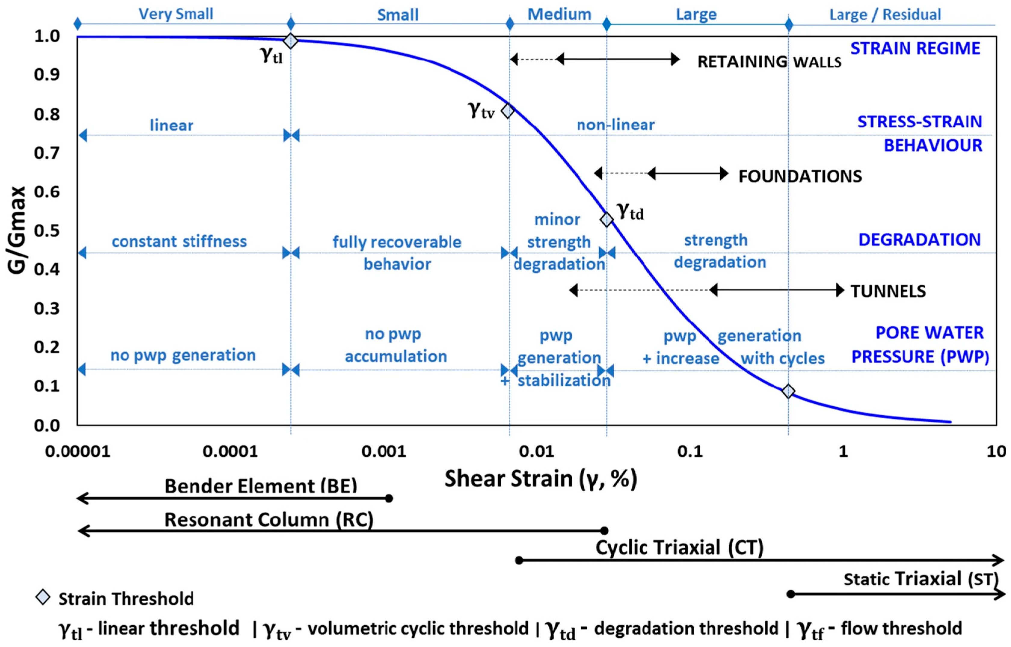
This equation determines the maximum shear modulus of soil layers in the field by applying in-situ methods that measure vs (e.g., the cross-hole or down-hole test, the seismic cone penetration test (SCPT) [8], and the spectral/multichannel analysis of surface waves (S/MASW) [9]). Furthermore, many studies have established empirical correlations from extensive laboratory testing data to estimate Gmax as a function of the void ratio and mean effective stress. The most commonly utilized equations are the ones introduced by Hardin and Richart [10] and Hardin and Black [11], and most recently by Wichtmann et al. [12] and Payan et al. [13]. Nevertheless, despite the potential advantages of these correlations, they can have a significant degree of variability and may not always offer an adequate representation of actual stiffness. Therefore, engineers should not solely depend on them in all situations. Nowadays, more reliable laboratory testing methods simulate (to an acceptable level) the shear loading conditions in the field, such as the resonant column and bender element tests [14,15]. The dynamic testing methods corresponding to different strain levels appear in Figure 2.
Once the shear strains in soils exceed a certain threshold level, the separation or slippage of intergranular contacts causes the behavior of the soil to become nonlinear, and the stiffness starts degrading until it reaches 5–10% of its original maximum stiffness at high strain levels. A modulus reduction curve represents this effect where the shear modulus decreases with increasing shear strain, as shown in Figure 2. Vucetic [16] defined two types of shear strain thresholds based on extensive cyclic laboratory data. The values of these thresholds depend on the soil type. The linear threshold () is the strain at which the ratio of the modulus to maximum modulus (G/Gmax) is 0.99, and before this threshold, the soil behaves elastically. Beyond this limit, the soil first behaves as a slightly elastoplastic material (nonlinear but still elastic) where permanent changes are negligible. Later, the strains increase to a second threshold, defined as the volumetric threshold shearing strain (), after which the soil microstructure undergoes an irreversible alteration, resulting in a permanent change in the stiffness of the soil. Investigations in [17,18,19] show that corresponds to a range of Gsec/Gmax between 0.60 and 0.85.
The secant shear modulus (Gsec) represents the ratio between the shear stress and shear strain at each loading step on the backbone curve (Figure 1), which refers to the one-way loading shear stress-shear strain curve. In other words, it is the slope of the line that connects the origin with the point along the backbone curve corresponding to (). For cyclic loading, the reduction in stiffness disappears after each turning point due to the re-engagement and interlocking of the previously slipped contacts between particles in the opposite direction. Naturally, if loading resumes back in this direction, elastic contacts will once again be lost, and stiffness will start degrading as before. Due to this nonlinearity and recovery of stiffness around load reversals, the stress-strain path forms a hysteresis loop, as presented in Figure 3a. The slope of the line that connects the endpoints of the hysteresis loop represents the “linear equivalent” shear stiffness of the soil, hence the secant shear modulus.
Figure 2.
Shear modulus degradation curve showing range classification, stress-strain behavior, type of degradation, and pore pressure state. The typical strain ranges related to different soil behavior and the laboratory equipment measurement range are also shown [20] (reprinted with permission from [Springer].
2.2. Damping Ratio
The damping ratio is an important dynamic property of soil. It represents the energy dissipation when waves propagate through the soil layers.
There are several types of damping in materials. However, we are only concerned with hysteretic and viscous damping in soils. These two types of damping occur due to different mechanisms. Hysteretic damping is independent of the vibration frequency and proportional to the displacement, while viscous damping changes with frequency and is directly proportional to the velocity.
During cyclic loading in soil, the damping behavior can be very complicated, and damping results from two main mechanisms, fluid flow loss and inelastic friction loss [21]. Soils dissipate energy even at very small strain levels [22]. At such strain levels where the soil is behaving elastically and no hysteretic loop will form, the fluids in the voids are responsible for the damping [23], which is an indicator that fluid energy loss is the dominant mechanism in small strain damping in soil (viscous damping). On the other hand, when exceeding the linear threshold (), where the behavior becomes nonlinear, the stress-strain curves exhibit a hysteresis loop as the soil is cyclically loaded. Beyond this threshold, hysteretic damping increases with the strain level (Figure 3b). Most energy dissipation is due to inelastic friction independent of the vibration’s frequency. Therefore, the nature of damping is hysteretic and viscous damping can be neglected [24,25].
Even though damping in the soil is known to be hysteretic, equivalent viscous damping often replaces it in most analyses due to mathematical simplicity. Viscous damping provides a very straightforward representation in dynamic analysis because it is linearly proportional to the velocity. Many geotechnical and structural dynamic problems approximate single- and multi-degree-of-freedom systems with a viscous dashpot, where damping force results as
where C = viscous damping coefficient, and = particle velocity.
“The equivalent viscous damping is determined in such a manner as to yield the same dissipation of energy per cycle as that produced by the actual damping mechanism” [26]. The damping ratio, D, represents the energy absorbed in one vibration cycle divided by the potential energy at maximum displacement in that cycle [27]. The equivalent damping ratio (D) due to hysteretic damping results from the following equation:
where AL = the area of the entire hysteresis loop (Figure 3a), and AT = the triangular area bounded by the secant modulus line at the point of maximum strain [28].
Small strain damping ratio (Dmin) often defies accurate measurement due to many factors, such as equipment damping and environmental noise. Therefore, Dmin varies over a broader range when measured by the resonant column method.
Xu et al. [29] presented a new method for measuring Dmin in the torsional shear test. The method examines the phase shift between the stress and strain signals and requires two calculation steps. The first step fits the sinusoidal time series of stress and strain signals to equations and determines the phase angle for both signals. The difference between and is the phase shift used for calculating the hysteretic material damping ratio. The Fourier transform method accurately computes the strain amplitudes by allowing the filtration of the signal’s frequency components. This method only applies to the elastic strain range of the material damping ratio (10−5–10−4%), where it shows accurate and consistent results.
Drnevich et al. [30] described two methods to measure the damping ratio in the RC test: (1) the steady-state vibration method (SSV) and (2) the free vibration decay method (FVD). The SSV method measures the input energy (current through coils) at resonance. The more input energy required to maintain a strain level translates to a higher damping value. However, the device cannot maintain precise resonance at high strain levels, and the decay method produces more reliable results over a short duration (~10 s) [31]. In the decay method, the power disconnects from the coils, allowing the sample to behave as a damped, freely vibrating system (Figure 4). The recorded decaying response then determines damping via the following equation:
where δ = logarithmic decrement, N = number of cycles, Z1 = first amplitude, Z1+N = amplitude after N cycles, and D = damping ratio.
For small values regarding the damping ratio as found in soil, can be approximated to 1, and the damping expression can be determined as follows:
According to Ray [31], N should be small when driving at high amplitude because a larger N would introduce strain effects due to a drop in amplitude by a factor of three over the measurement interval. ASTM D4015 [32] suggests the use of fewer than 10 cycles. The research by Gabryś et al. [33] on the RC apparatus agrees with these regulations. Furthermore, a recent study by Mog and Anbazhagan [34] examined the effect of the number of successive cycles (N) used in calculating the damping ratio using the (GCTS) resonant column apparatus. When measuring up to 10 cycles, they reported an increase in the damping ratio when increasing the number of cycles. Nevertheless, after 10 cycles, the damping ratio diminishes for higher numbers of cycles in the measurements (i.e., for 20, 30, and 50 cycles). Due to the considerable scatter in the damping ratio measurements determined by this method, estimates should use two or three successive cycles to calculate the damping ratio in the RC test.
The SSV method for calculating the damping ratio is also called the half-power bandwidth method. It initially determined a structure’s modal damping ratio ξ from the width of the peaks in its frequency response function, and it may apply to soil in the RC test. In this method, the width of the frequency response curve near the resonance determines the logarithmic decrement (). The half-power bandwidth (∆ω) is the width of the peak where the magnitude of the frequency response function is multiplied by the peak value [35]. The following equation calculates :
where f1 and f2 = frequencies below and above the resonance corresponding to strain amplitude = P, Pmax = maximum amplitude (or resonant amplitude), fr = resonant frequency (Figure 5), and D = damping ratio.
When the damping is small and the amplitude is P = , Equation (6) can be written as
Then, the damping ratio becomes
The scatter (from an average value) of the damping ratio measured using the SSV method and FVD method with two successive cycles can reach 15% (of the average) at strain levels less than 0.005% [34] and even higher (up to 50% of the average) when the number of successive cycles is higher (3, 7, and 10 cycles). The ambient noise during the RC test may cause this difference [36] and/or the number of applied cycles (higher for SSV). Several authors suggested relying on SSV (half-power bandwidth) to determine the damping ratio within a very small shear strain range where the frequency response curve is still symmetrical. The frequency response curve becomes non-symmetric at higher strain levels (>0.005%), and measurement accuracy is uncertain. Therefore, the FVD method better estimates the damping ratio at high strains [37,38].
In order to overcome the inaccuracy of the FVD method due to the ambient noise and a limited number of data points, Xu et al. [29] adopted Hilbert transform to analyze the decayed signal. This method finds the instantaneous frequency and amplitude of the signal (envelope), significantly increasing the number of data points. An exponential function fits the instantaneous amplitude as follows:
where is the shear strain, t is time, a is a fitting constant, and b is a fitting parameter that represents the decay of the instantaneous amplitude.
Based on Equation (9), the logarithmic decrement becomes
At very small strains where frequency degradation does not occur, the instantaneous frequency (f) remains constant in Equation (10). Therefore, this method is only suitable for measuring the low strain damping ratio (Dmin).
3. Device Performance in RC-TOSS Testing
3.1. Fundamental Concepts
The resonant column test uses a high-accuracy accelerometer to acquire readings at very small strains (10−4%). At these strain levels, the shear modulus behaves as linear elastic (Gmax). The relationship between the acceleration, velocity, and displacement experiencing harmonic motion produces accuracy at such low strain values. Differentiating the expression for simple harmonic displacement (u) produces expressions for velocity () and acceleration ():
where A = the displacement amplitude, = the circular frequency, and t = time.
The two vital elements in resonant column testing are the accelerometer’s sensitivity and the range of typical resonant frequencies produced by the device. A high-quality piezoelectric accelerometer produces about 300 millivolts/g. A high-grade digital voltmeter can easily measure up to 0.1 millivolt AC, translating to acceleration as < 0.01 g. The same meter could also detect frequencies/periods of dynamic signals with four- or five-digit accuracy. Typical resonant frequencies would range from 200 < < 500 rad/s. The frequency range is a significant advantage in producing small strains. Assuming that the specimen length is L = 0.14 m, and, at resonance, for a natural circular frequency of = 400 (rad/s), then acceleration = 0.025 (m/s2). From Equation (13), displacement u = 1.56 × 10⁻⁷ m, and the shear strain follows that
Based on the wave propagation theory in rods, the resonant column test applies a torsional oscillation on the top of the specimen. The testing procedure follows the standard designated ASTM D4015-81. However, the standard does not include sample preparation for a hollow cylinder specimen. Therefore, this review describes the device and testing procedure. Ishimoto and Iida [39] developed the first resonant column testing system. Hollow cylindrical samples produced more uniform shear strains within the cross-section of the specimen [40,41,42]. More history of the RC test is presented by Woods [43]. The device today can consistently measure stiffness at small-to-intermediate (up to 10−1%) strain levels, making it one of the most used laboratory devices for measuring the dynamic behavior of soil.
The fixed-free configuration oscillates the soil specimen at the top end while it fixes the base. The driving frequency gradually increases to find resonance, and the accelerometer measures the specimen’s response. The frequency that maximizes the response amplitude is the first mode fundamental frequency of the sample (resonant frequency). By using the wave equation and theory of elasticity and considering the fixed-free configuration of the device, the governing equation becomes
where I = the sample polar moment of inertia, I0 = the free end mass polar moment of inertia, Vs = the shear wave velocity in the sample, 𝜔𝑛 = resonant frequency in torsion, and L = the length of the sample.
The specimen’s geometry and mass determine the value for I, and I0 comes from calibrating the drive head (steel top ring, magnets, and mounting plate) using the three-wire pendulum method so can be computed. Subsequently, we can relate the resonant frequency to the shear wave velocity:
The measured shear wave velocity and specimen mass density produce the shear modulus via Equation (1).
The torsional simple shear test applies torque to the specimen using a drive system of two magnets and four coils. The current flowing through the coils relates directly to the magnitude of torque. Calibration relating current flow to torque using a specimen rod of known stiffness provides the proper conversion factor. Proximitors, mounted near the specimen’s top, measure displacements that translate to rotation () at the top of the specimen. For the fixed-free configuration, the rotation () varies linearly with the height of the measuring point in the specimen, starting from zero at the bottom and ending with the maximum value at the top. In our device, the shear strain relates to top rotation via the following equation:
where = the rotation (Equation (18)), h = height of the cross-section of interest, and r = the radial distance between the specimen axis and the calculated point (Figure 6).
where x = arc length where a point at the edge of the specimen rotates, R = radius of the specimen, = displacement of the attached accelerometer, and = radial offset of the accelerometer from the specimen axis.
As an additional advantage, this device uses the same drive system for the RC and TOSS tests, so both can be applied interchangeably during a testing sequence. The tremendous advantage here is that a small strain test (RC) may be performed before and after any TOSS stage (cyclic or irregular history), providing an index value of Gmax throughout the test sequence.
The RC test requires displacement measurements with very high accuracy at very low amplitude ( = 10−4%), provided by an accelerometer mounted on the drive head and connected to a multimeter and oscilloscope, providing dynamic amplitude and frequency data. For the TOSS test, two proximitors mounted on the measurement post measure rotational displacement. Since the proximitors measure the air gap between themselves and a metal target, they do not touch or impede the motion of the drive head. The RC test is highly accurate, measuring small-to-medium strain levels between 10−4% and 10−2%. The TOSS test is more suitable for studying the dynamic behavior under medium-to-large strains ranging from 10−2% to 1%.
The main difficulties encountered when conducting dynamic torsional testing are related to sample preparation. Shear modulus and damping ratio measurements are very sensitive to the void ratio. In order to study the effect of loading conditions on soil, we need to form several hollow cylindrical soil samples with the same initial void ratio. This can be challenging to achieve, and any slight inaccuracy in measuring the initial density of the sample causes misleading results. Other problems may appear during setting up the device for testing. An insufficient vacuum between the mold and membrane causes nonuniformity in the sample. Extra care is required when fixing the drive head on the top of the sample to ensure good contact between the soil and the porous stone. If any disturbance in the sample is noticed after removing the molds, the procedure should be repeated, costing the researcher hours of work.
3.2. Advantages and Disadvantages
The hollow cylinder specimen configuration produces a uniform strain field with fewer end effects than a triaxial or simple shear device. With an inner diameter of 4 cm and outer diameter of 6 cm, the variation in shear strain with radial distance remains +/− 20% of the average strain. As discussed later, small voids and inclusions do not significantly change the specimen properties since there are no critical points in the connection between the device and the specimen. Any imperfections are averaged over the entire specimen cross-section and length. The primary strain mode is horizontal shear, which is ideal for site response analysis. RC tests range in strain over five orders of magnitude, while TOSS tests can measure four orders. The RC tests are uniform cyclic; however, the TOSS tests may be uniform, cyclic with static offset, or entirely irregular and arbitrary. As an additional advantage, this device uses the same drive system for RC and TOSS tests, so both can be applied interchangeably during a testing sequence. The tremendous advantage here is that a small strain test (RC) may be performed before and after any TOSS stage (cyclic or irregular history), providing an index value of Gmax throughout the test sequence.
The disadvantages include increased specimen preparation complexity, lower confining pressure ranges (air must be used and confining fluid), and a less robust testing frame. The device will not load a specimen to complete plastic failure. Saturated specimens may be tested, but most work is performed in dry or unsaturated conditions. Table 1 lists the pertinent features, advantages, and disadvantages of the testing method.
4. Factors Affecting the Dynamic Behavior of Soil
Many researchers have assessed the effects of different soil properties on the dynamic behavior of soil. Some factors did not affect behavior, while others influenced behavior significantly and were included in empirical equations to calculate the shear modulus and damping ratio. Hardin and Drnevich [40] divided the factors that influence the dynamic behavior of soil into three categories: very important, less important, and relatively unimportant. For dry sand (the soil tested in this investigation), the strain amplitude, effective confining pressure, and void ratio significantly influence dynamic properties. The degree of saturation, the over-consolidation ratio, and loading frequency contribute very little to behavior. However, for other soils, saturation, OCR, and other parameters may significantly influence Gmax, G, and D. They considered that the number of loading cycles did not influence the shear modulus of sand. [40]. However, the TOSS tests in this study show a rather substantial effect. The following sections present the impact of these parameters on sand behavior.
4.1. Strain Amplitude
4.2. Magnitude of the Effective Confining Pressure
Hardin and Richart [10] studied the influence of effective confining pressure through a laboratory testing program. They found that the shear modulus increases and the damping ratio decreases with increasing effective mean principal stress. In a following study on clean sand by Hardin and Drnevich [40], they concluded that for very small strain amplitudes, the modulus (Gmax) varies with the 0.5 power of mean effective principal stress. For larger strains, the modulus depends on soil strength with a variation approximately equal to the 1.0 power. Later studies also confirmed this observation [47,48,49,50,51,52], where the power (n) in Equation (21) ranged between 0.45 and 0.62.
A recent study [34] on the RC device agrees with the previous studies, where the damping ratio decreased with increasing confining pressure due to the higher contact between the particles, decreasing the attenuation of the propagating wave.
4.3. Duration of the Effective Confinement Pressure
Stokoe and Richart [53] conducted laboratory and field tests to find the effect of the duration of confining stress on the shear modulus under low-strain conditions (Figure 7). Darendeli [54] confirmed their results, where G increased with time at each applied confining pressure during testing. However, this effect was marginal for sandy soils at confining pressures lower than 200 KPa. Darendeli [54] also found that Dmin decreases as the specimen consolidates at a given confining pressure. Note that both increase linearly with the log of time.
4.4. Number of Loading Cycles
The studies in [55,56,57,58] observed that the number of cycles does not affect the shear modulus below the elastic threshold strain, usually in the range of 0.001% to 0.01%. Thus, the value of Gmax is considered independent of the time of vibration.
After exceeding the cyclic threshold, most studies reported an increase in the shear modulus with the increasing number of cycles for dry or drained sand under cyclic loading, called “cyclic hardening in stiffness”. Nevertheless, the studies have not entirely agreed on the degree of this effect, whether slight or significant. The increase is significant for the first 10 cycles, followed by a relatively small change [59]. For Sherif and Ishibashi [41], the increase in the shear modulus reached up to 28% at the 25th cycle and then leveled off. Several factors influence the cyclic hardening in stiffness: fabric reorientation, particle relocation, and an increase in contact area [31]. They reported the highest increase in the shear modulus of about 5% per logarithmic loading cycle. RC-TOSS tests obtained similar results where the increase was up to 120% of the initial value at a given strain level, and the increase was proportional to Log N (number of cycles) [60]. The damping ratio could drop to 50% of its initial value after 200 cycles [60].
Several authors found a decrease in damping with the number of cycles [23,59,61]. The RC-TOSS tests conducted by Ray and Woods [60] showed a more pronounced reduction in damping ratio at a higher strain and a continuous decrease in damping on a Glacier Way Silt specimen after 30,000 cycles without an indication of leveling off.
Cherian and Kuma [62] conducted resonant column tests on sand specimens with relative densities of 61 and 85% at confining stresses of 300 and 500 KPa to study the effect of vibration cycles on the dynamic properties. After 1000, 10,000, and 50,000 cycles at different strain levels, the measurements showed no effect below a certain threshold (shear strain between 0.0024 and 0.0044%). However, at higher strain levels, additional cycles caused an increase in the strain magnitude, causing a decrease in shear modulus and an increase in damping ratio. The strongest influence occurred at a confining stress of 300 KPa, a relative density of about 61%, and a shear strain amplitude of 0.03%. After 50,000 cycles, they produced an increase in shear strain of 34%, leading to an 8% decrease in the shear modulus and a 10% increase in the damping ratio.
Another study on the pre-vibration effect on the dynamic properties of dry Toyoura sand was carried out by Yang et al. [63]. They improved their energy-injecting virtual mass (EIVM) resonant column system (Mark II) to reduce the time needed to reach a steady-state vibration. The system achieved a steady state after 12 equivalent cycles, minimizing the disturbance to the specimen. The air pluviation method made cylindrical specimens at 38 mm in diameter and 81 mm in height to achieve a relative density of 65%. Different sets of tests received pre-vibrations of 0.001, 0.005, 0.02, and 0.05% for 100–100,000 cycles and confining stresses of 25–500 KPa. The test results showed that the elastic threshold strain was about 10−2, where the pre-vibration did not affect the soil’s dynamic properties. Less than a 5% decrease in the maximum shear modulus occurred when the specimen was pre-vibrated at a strain up to 0.02% for 100,000 cycles. Pre-vibrations of less than 10,000 cycles produced a marginal decrease. This pattern inverted when the pre-vibration increased to 0.05%, as the maximum shear modulus increased by 10% with the number of cycles (=100,000). The trend found by Yang et al. [63] appears in Figure 8. Furthermore, the study shows a negligible effect of the confining pressure on the influence of pre-vibration (less than 3%).
4.5. Loading Frequency
Hardin [24] and Hardin and Black [11] conducted precise static torsional and resonant column tests. They observed that frequency had no influence on the low-strain shear modulus (Gmax). As a result, the static and dynamic tests produced identical Gmax results due to the elastic behavior of the soils at very small strain levels.
At higher strain levels, strain-rate effects become more evident. Stiffness increases with higher strain rates (RC-TOSS) when compared to monotonic static tests with low strain rates [64,65]. The cyclic torsional test is usually conducted at frequencies between 0.1–1 Hz, while in the resonant column test, the resonant frequency ranges from 30–200 Hz. Ray and Woods [60] concluded that the two tests are interchangeable, provided that the cyclic effects have no significant impact. Nevertheless, Tatsuoka et al. [66] and Lo Presti et al. [67] found that the trend in a monotonic test is different (shear strain rate of 0.01% per minute). It produces lower shear stiffness for a specific strain level, so the G/Gmax- curve should be evaluated separately for monotonic and cyclic loading conditions.
The loading frequency above 1 Hz significantly affects sandy clay’s minimum damping ratio (Dmin), as it can increase by 100% over a log-cycle increase in excitation frequency [54]. However, studies show that the damping of sand is independent of the frequency.
4.6. Void Ratio
Soil void ratio is a fundamental property that significantly affects the maximum shear modulus (Gmax). The shear wave velocity decreased linearly with the increasing void ratio in [10]. Since the 1990s, researchers have introduced different empirical correlations for Gmax as a function of the void ratio (F(e)) for different types of soils by fitting equations to laboratory test results, as described in Equation (21). All studies confirmed that the small strain shear modulus decreased with an increased void ratio.
Most correlations represent the maximum shear modulus as a function of the void ratio and confining stress as follows:
This equation is normalized for the atmospheric pressure as follows:
where A, a, and n are experimentally determined coefficients and are called intrinsic (state-independent) parameters and are associated with small strain stiffness [68], equals the mean effective stress in [KPa], is the atmospheric pressure [KPa], and F(e) is the function of void ratio, which varies from researcher to researcher [69,70,71,72,73,74,75,76,77]. The parameters proposed by studies on sand are summarized in Table 2.
Wichtmann et al. [12] have developed the most recent empirical equation based on their extensive laboratory testing. It depends on the uniformity coefficient (CU) and the percentage of fine particles (FC). The parameters A, a, and n in Equation (21) for sands with non-cohesive fines (for FC < 10%) are as follows:
The void ratio did not affect the modulus degradation curve G/Gmax based on RC-TOSS test results on Toyoura sand [78]. Researchers have attempted to find a correlation between void ratio and strain-dependent shear modulus, such as Oztoprak and Bolton [79], who evaluated 454 tests on 60 soils from 65 reference studies. As a result, they modified Equation (21) and suggested a different void ratio function for strain-dependent stiffness:
where A and n are the strain-dependent parameters given in Figure 9, as determined by Oztoprak and Bolton [79].
This equation has a relatively large scatter indicating the difficulty of obtaining a correlation for the strain-dependent shear stiffness that would be reliable for a wide variety of granular soils. Therefore, a different approach can model the dynamic behavior of soil at larger strain levels.
Payan et al. [13] conducted RC tests on 11 types of sand to study the effect of particle shape and gradation on the small strain damping ratio (Dmin). The proposed correlation (Equation (27)) is a function of the regularity (p) of the particles, which is the average of roundness (R) and the sphericity (S) obtained from the particle shape characterization chart by [80].

Table 2.
Correlations for small strain shear modulus Gmax of sand using Equation (21). Gmax is in [MPa], in [KPa], and = 1 atm.
Table 2.
Correlations for small strain shear modulus Gmax of sand using Equation (21). Gmax is in [MPa], in [KPa], and = 1 atm.
| Soil Tested | D50 [mm] | CU [−] | A [−] | F(e) [−] | n [−] | Reference |
|---|---|---|---|---|---|---|
| Ottawa sand No. 20–30 | 0.72 | 1.20 | 69 | 0.5 | (Hardin and Richart, 1963) [10] | |
| Ticino sand (subangular) | 0.54 | 1.50 | 71 | 0.43 | (Lo Presti, et al., 1993) [81] | |
| Toyoura sand (subangular) | 0.22 | 1.35 | 72 | 0.45 | (Lo Presti, et al., 1993) [81] | |
| Quiou carbonate sand | 0.75 | 4.40 | 71 | 0.62 | (Lo Presti, et al., 1993) [81] | |
| Kenya carbonate sand | 0.13 | 1.86 | 101–129 | 0.45–0.52 | (Fioravante, 2000) [48] | |
| Ticino sand (subangular) | 0.55 | 1.66 | 79–90 | 0.43–0.48 | (Fioravante, 2000) [48] | |
| Hostun sand (angular) | 0.31 | 1.94 | 80 | 0.47 | (Hoque and Tatsuoka, 2000) [82] | |
| H.River sand (subangular) | 0.27 | 1.67 | 72–81 | 0.50–0.52 | (Kuwano and Jardine, 2002) [83] | |
| Glass ballotini (spheres) | 0.27 | 1.28 | 64–69 | 0.55–0.56 | (Kuwano and Jardine, 2002) [83] | |
| Silica sand (subangular) | 0.20 | 1.10 | 80 | 0.5 | (Kallioglou, et al., 2003) [84] | |
| Silica sand (subangular) | 0.20 | 1.70 | 62 | 0.5 | (Kallioglou, et al., 2003) [84] | |
| Silica sand (subangular) | 0.20 | 1.10 | 62 | 0.5 | (Kallioglou, et al., 2003) [84] | |
| Silica sand (angular) | 0.32 | 2.80 | 48 | 0.5 | (Kallioglou, et al., 2003) [84] | |
| Toyoura sand (subangular) | 0.16 | 1.46 | 71–87 | 0.41–0.51 | (Hoque and Tatsuoka, 2004) [49] | |
| Toyoura sand (subangular) | 0.19 | 1.56 | 84–104 | 0.50–0.57 | (Chaudhary, et al., 2004) [50] | |
| Ticino sand (subangular) | 0.50 | 1.33 | 61–64 | 0.44–0.53 | (Hoque and Tatsuoka, 2004) [49] | |
| Silica sand | 0.55 | 1.80 | 275 | 0.42 | (Wichtmann and Triantafyllidis, 2004) [51] | |
| SLB sand (subround) | 0.62 | 1.11 | 82–130 | 0.44–0.53 | (Hoque and Tatsuoka, 2004) [49] | |
| Natural quartz sand | 0.27–1.33 | 1.34–2.76 | −5.88 Cu+57.1 | 0.47 | (Senetakis et al., 2012) [85] | |
| Quarry sand | 0.16–2 | 2–2.5 | −9.54 Cu+78.1 | 0.63 | (Senetakis et al., 2012) [85] | |
| Volcanic sand | 0.23–1.6 | 1.53–4.18 | −3.04 Cu+52 | 0.55 | (Senetakis et al., 2012) [85] | |
| Blue sand | 1.01–1.94 | 1.41–8.22 | (Payan et al., 2016) [13] | |||
| Danube Sand | 0.107–0.424 | 2.06–9.85 | 62 | 0.45 | (Szilvágyi, 2017) [52] |
Szilvágyi (2017) [52] compared his measurement data on Danube sand to the correlations proposed by Carraro et al. (2009) [68], Biarez and Hicher (1994) [86], Wichtmann and Triantafyllidis (2009) [12,87] Wichtmann, et al. (2015) [12], and Oztoprak and Bolton (2013) [79]. The fit was excellent for Carraro et al. (2009) [68], as 75% of the measured Gmax values fell within the range of ±15%. Furthermore, 87% of the data points were within the range of ±20%. The correlation provided by Biarez and Hicher (1994) [86] produced satisfactory outcomes for the soils examined. Among the 69 measured Gmax values, approximately 72% were found to fall within the ±15% range using this correlation. Moreover, around 84% of the data points were within the ±20% range. The correlation for clean sands (Wichtmann and Triantafyllidis, 2009) [87] tends to over-predict many measured results. A total of 47% of the data points lie within the ±15% margin, and 60% of data points lie within the ±20% margin. In contrast, the correlation provided for sands containing non-plastic fines by Wichtmann et al. (2015) [12] underestimates the Gmax of soils with low content of plastic fines (up to 7.6%). The accuracy of the correlation is similar to the previous equations, with approximately 51% of the data points falling within the ±15% margin and around 63% within the ±20% margin. However, it should be noted that these equations underestimate Gmax in certain cases by more than 35%. The correlations provided by Oztoprak and Bolton (2013) [79] tended to overestimate the majority of the measured results. However, the estimated values still fell within the range of ±100%, which was also observed by the researchers for a significant portion of the collected data.
4.7. Effect of Sample Disturbance
In a study by Szilvágyi et al. [88], in-situ and laboratory tests were conducted to measure the shear wave velocity for soils in Budapest, Hungary, to use it for 1D ground response analysis. They compared shear wave velocity values obtained using RC and TOSS measurements to the multichannel analysis of surface waves (MASW) and seismic cone penetration tests (SCPT). The shear modulus obtained from the laboratory measurements provided a lower bound for the in-situ tests, as shown in Figure 10. The author justifies this difference because the field void ratio (state of compaction) and stress state are not certain. Two later studies agreed with these findings [89,90]. In both studies, in-situ seismic dilatometer Marchetti test (SDMT) measurements showed a higher Gmax than those obtained from the RC test by 17% to 46% in [89] and by 8% to 35% in [90]. The decrease in the shear modulus defined in the laboratory can be a cause of the effect of soil suction or disturbance during sample preparation.
Lashin et al. [91] compared resonant column small strain shear modulus measurements with the stiffness obtained using the piezoelectric ring-actuator technique (P-RAT). This device recorded the shear wave velocity of the soil based on the transmission of a mechanical signal through the soil specimen with source and receiver transducers during the oedometer test. The testing program included tests on sand specimens prepared using the wet-tamping method with different void ratios and confining pressures. The results demonstrated higher values for the shear wave velocities measured by the RC tests compared to the P-RAT, especially for loose samples. The authors attributed this overestimation to the discrepancy between the assumption of the linear elastic behavior of soil and natural soil behavior. The study recommends using the P-RAT technique to study the small strain stiffness of soil due to its higher accuracy.
4.8. Temperature Effect
Yu et al. [92] used a special resonant column apparatus (RCA) to study the dynamic behavior of frozen silt soils, where a cooling bath (Thermo Scientific HAAKE Bath, Waltham, MA, USA) controlled the specimen temperature to ±0.01 °C. The sample was compacted, placed in a chloroprene rubber membrane, saturated, and confined in silicon oil. The study showed that the stiffness and damping ratio remained constant with temperature until −1.4 °C. The properties started to increase considerably until −3 °C (sensitive range), and at colder temperatures, the change was gradual (insensitive stage). The maximum shear modulus for the frozen soil was much higher than at ambient temperature. The shear modulus degradation curves reached lower values at low temperatures when compared to soils at ambient temperatures. For instance, at a strain level of 10−3%, the value of G/Gmax was 40% for a sample tested at a temperature of −15 °C, whereas it was 90% for a sample tested at room temperature. However, the damping ratio continued increasing as the temperature dropped for strains of 10−6 to 5 × 10⁻⁴, as shown in Table 3 and Figure 11. The authors suggested temperature correction coefficients based on the RC tests to modify the dynamic properties and account for freezing effects.
4.9. Soil Improvement Effect
Various techniques can enhance the dynamic characteristics of sand, and several investigations have examined the impact of various additives on a sand by testing the soils in torsion.
Das and Bhowmik [93] measured the shear modulus and damping ratio of Barak River sand mixed with crumb rubber in different rubber/sand ratios (1, 2, 3, 4, and 5%). The specimens were compacted in three layers by a tamping rod before testing in the resonant column apparatus. The study reported an increase in the shear modulus when increasing the rubber content to 3%, where the shear modulus increased by up to 2.12 times. The shear modulus decreased beyond the 3% ratio, as shown in Figure 12a. The damping ratio behaved in the opposite manner, where it decreased as rubber content rose until it reached 3%, then increased again. The most significant decrease in the damping ratio (1/2.63) occurred at a 3% rubber/sand ratio.
Microbial-induced biopolymers provide a sustainable alternative to cement soil treatment for improving static strength and hydraulic conductivity. However, this is not necessarily the case for dynamic properties. Im et al. [94] measured the dynamic properties through resonant column tests of Jumunjin sand mixed with a gellan gum solution (gum/sand 1–2%). In most testing conditions, the maximum shear modulus decreased after mixing the sand with the binder (except for the 2% binder dried condition and 1% binder with confining stress of 25 KPa). The shear modulus reduction curve also decreases at a higher rate at low strains for the mix. The stiffness decreases at higher confining stress, indicating that the bonds break between the sand and binder particles. Furthermore, the rigid sand grains and ductile gellan gum dissipate significantly more energy, as reflected by the high damping ratios.
The same study tested another binder [94], xanthan gum, with a 1% gum/sand content. In this case, the additive increased in Gmax for all confining stresses; however, the secant shear modulus reduced at strain levels lower than the untreated soil. The energy dissipation was even higher than the gellan gum, possibly due to the excessive structural disturbance of the mixing interface.
Li et al. [95] substituted steel slag for cement as the stabilizing additive. Steel manufacturing produces large slag volumes as a byproduct, requiring proper disposal if it is not reused. They conducted resonant column tests on a slag sand mixture (SSM) with a slag/sand content of 20, 30, 40, and 50% at a water content of 15% mass compared to cement/sand specimens mixed at 8, 12, and 15% cement. The 5 cm (in diameter) by 10 cm (in height) cylindrical specimens were mixed, compacted, and tamped into four layers, then left to cure for 1, 3, and 7 days before running the tests. The study reported an improvement in the maximum shear modulus with the increasing steel slag content up to 40%, which starts decreasing again. At the optimum slag steel content (40%), it was adequate for all the particles to be involved in the hydration reaction. The optimum steel slag produced a Gmax nearly identical to the Gmax from the cement/sand samples (15%), as shown in Figure 13a. With increased curing time, the SSM specimens achieved a higher shear modulus.
Similarly, the energy dissipation represented by the damping ratio initially increased with the increasing steel slag content peaking at a 40% ratio before declining, as shown in Figure 13b. The damping behavior may be due to the coating of the steel slag particles on the contact areas between the sand particles. Confining pressure effects produced significant changes in shear modulus but influenced damping very little.
Basas et al. [96] studied the improvement of dynamic properties by injecting sand specimens with Portland cement grout. Clean sand specimens (50 mm in dia. and 112 mm in ht.) received grout injections with water/cement ratios of 1, 1.25, 2, 2.5, and 3 (stable to unstable suspension). The specimens required 24 h to cure. Torsional and flexural resonant column tests were used to determine the shear modulus and damping ratio. The confining pressure applied to the specimens produced only a marginal effect on the dynamic properties. The water/cement ratio created the most significant changes to the shear modulus. Grouting increased the shear modulus by (20–30%) for limestone sand and 45% for Ottawa sand when the water/cement ratio was reduced from 3 to 2. The shear modulus increased further (60–70%) for the limestone and 55% for the Ottawa sand when the water/cement ratio was lowered from 2 to 1. When compared to clean sands, grouting with stable suspensions improved the shear modulus by 36 times at low confining pressure (σ3 = 50 kPa) and 11 times at higher pressure (σ3 = 400 kPa) as shown in Figure 14. Grouting decreased soil damping at low strain levels (below 10−3) by one-seventh. At higher strain levels, on the other hand (above 10−2%), the clean sand showed damping ratio values higher than the grouted sand.
Mixing sand with rubber particles may improve compressibility, durability, and seismic isolation. In order to estimate the dynamic properties of this composite material, Wu et al. [97] conducted resonant column tests on Fujian sand mixed with rubber particles produced from recycled waste tires. In this study, the specimens contained 0–100% rubber particles. (all sand–all rubber). The study showed a significant decrease in the maximum and secant shear moduli (Gmax and Gsec) with increased rubber content. Moreover, the damping ratio increased with increasing rubber content at low shear strain levels (6 × 10⁻⁴ to 1 × 10⁻³), and then it exhibited lower values than the clean sands for higher strain levels, as shown in Figure 15.
5. Soil Models
The complexity of the dynamic behavior and its dependency on various factors and soil properties motivated the use of soil models to simulate the shear stress-strain curves. Any change in the initial soil matrix (e.g., size, shape, and orientation) may have a considerable effect on the behavior. This makes it very difficult to produce one equation that takes into account all of these factors. After obtaining the curve-fitting constants of the employed soil model using regression analysis, the model coupled with the Masing criteria can perform very well, simulating the shear stress-strain curve when the soil is subjected to cyclic and irregular loading histories. The main limitations of such models are the need for dynamic laboratory test data in addition to the incapability to simulate stiffening behavior with an increasing number of cycles.
5.1. Irregular Loading and Masing Criteria
A simple soil model can easily simulate soils’ nonlinear monotonic shear stress-shear strain behavior. However, predicting such behavior for reversible strains and irregular load histories requires introducing more rules that dictate the path followed by the shear stress-shear strain curve when generating the hysteresis loops.
Masing [98] investigated the behavior of brass under cyclic loading and introduced two rules that are sufficient to describe regular, symmetric cyclic loading and could be applied to soils, as discussed by Pyke [99]:
- The shear modulus in unloading is equal to the initial tangent modulus for the initial loading curve (Figure 16);
- The unloading and reloading curve duplicate the initial curve, except that its scale increases by a factor of two in both directions. The variables τ and γ in the formulation are replaced by (τ − τi)/2 and (γ − γi)/2 (Figure 16).
Note that these two rules are insufficient to describe the soil behavior if the loading is more general or irregular (not symmetrical or periodic). Jennings [100] presented a general nonlinear hysteretic force-deflection relation for a one-degree-of-freedom structure to study the earthquake response of a yielding structure, and he extended the criteria by adding two additional rules, as follows:
- 3.
- Unloading and reloading curves should follow the initial curve if the condition exceeds the previous maximum shear strain;
- 4.
- If the current loading or unloading curve intersects a previous one, it should follow the previous curve.
Most researchers cite these four rules as the extended Masing criteria, which were first used for soil in [101,102] and today extend to soil models that formerly described only monotonic behavior. Figure 17a illustrates an example using the Ramberg-Osgood model.
As Valera et al. [103] mentioned, the two added rules require that the model keeps track of previous paths in both directions. Programmed turnaround co-ordinates use a last in-first out (LIFO) sequence to determine when the stress-strain curve applies rule (4).
Figure 17b illustrates the discussion by Pyke [99], where he shows the stress-strain curve transitioning from point 4 as a turnaround to point 2. The transition occurs at point 3. Upon reloading from point 4, the solution suggested by Rosenblueth and Herrera [104] and that proposed by Jennings [100] would follow path A. On the other hand, if the dashed curve 0–1 is the greatest previous reloading curve, it would follow stress path B.
5.2. Modified Ramberg-Osgood Model
Ramberg and Osgood [105] proposed a model with three parameters describing the stress-strain curves of aluminum alloy stainless-steel and carbon-steel sheets to consider the gradual transition from the straight elastic line for low loads toward the horizontal line characterizing plastic behavior. Jennings [100] used this model to describe the hysteretic curves for the steady-state response of yielding structures as a relationship between displacement and restoring force. Then, this model was first used for soil by Faccioli et al. [106] to describe the stress-strain nonlinear behavior of the soil under simple shear in their one-dimensional wave propagation model to study the seismic response in Managua. The form today differs from the original, and the model used for soil in geotechnical earthquake engineering was demonstrated by Streeter et al. [107], as shown in Equation (28). This equation has been widely used in several studies, e.g., [52,60,108]. The formulation used for the shear stress-shear strain relation follows:
where is the shear strain, is the shear stress, Gmax is the small strain shear modulus, is the maximum shear strength (usually from triaxial tests), and are the curve-fitting constants.
It is a straightforward calculation to obtain shear strains from shear stresses. However, it is more difficult to invert the formulation. Different methods can solve this problem, including the Newton-Raphson method.
The secant shear modulus, as defined by the ratio between the shear stress and shear strain at any strain level, can be expressed in the RO model as follows:
The following equation gives the tangent shear modulus:
Subsequently, Equations (29) and (30) produce shear modulus degradation for secant and tangent shear moduli, respectively. Note that the secant shear modulus is always higher than the tangent modulus at any given strain, as shown in Figure 18.
It is common to use a log scale to plot strains on the horizontal axis to see the soil behavior more clearly. Researchers may express strain either in percent (%) or (mm/mm), and the modulus may reduce significantly below its maximum value at relatively low strain levels ( = 0.001).
Equation (28) has a dimensionless form by introducing a reference shear strain which is based on and Gmax as follows:
The maximum shear stress is typically assumed to equal the Mohr-Coulomb failure envelope strength with effective stress properties, as shown in Figure 19. Based on the diagram, the maximum shear strength is
Equation (35) applies to the isotropic confining conditions often produced in laboratory tests. Equation (36) represents anisotropic (K0) conditions in the field. The dimensionless form (Equation (33)) applies to the soil at any depth. Changes in automatically resolve the soil’s depth effects (confining stress). Normalizing the curves produces one standard curve for one soil type in the profile.
When considering loading reversals, the formulation becomes slightly more complex. The most straightforward approach uses the Masing formulation and substitutes into the equations for , and for ; then, the formulation becomes
where and equal the shear strain and shear stress at the last turning point.
The same substitution occurs in formulations for Gsec and Gtan (Equations (29) and (30)). This approach will produce a hysteresis loop with reversals, as shown in Figure 20. The figure illustrates some other important properties as well. At every reversal point, the stress-strain curve starts with a stiffness of Gmax. The line labeled Gsec shows an example of computing the secant modulus for a hysteresis loop (Figure 3a).
Damping in the Ramberg-Osgood model is calculated by integrating along the stress axis. Given the differential element shown in Figure 20, it has a width of dτ and a length of (γ2 − γ1).
We can integrate this expression from τ1 to τ2. The two functions can be written as
If , then
If then .
Then, the integration can be written as
The final formula resulting from the integration is given by
Subsequently, from the definition of the damping ratio, it is calculated by using the following equation:
Midas uses a different form of the Ramberg-Osgood equation with two curve-fitting constants instead of three. The initial loading moves along the following skeleton curve [109].
where G0 is the initial stiffness (shear modulus), and , and are the model parameters given by
is the reference shear strain, and ℎ𝑚ax is the maximum damping constant. For unloading and reloading, the hysteresis curve is as follows:
where and are the shear strain and stress values at the turnaround point.
Considering the uniaxial condition, the hysteresis curve is expressed as follows:
In 3D conditions, the formula divides into hydrostatic and deviatoric (shearing) components. The formula becomes a 3D expression:
where E0 is the initial stiffness and is the von Mises stress.
If the equivalent deviatoric strain , it is expressed as follows:
The following equation calculates the tangent stiffness:
The Poisson’s ratio is assumed to be a constant regardless of the stress state, and Equation (49) provides the equivalent elastic modulus. The 3D stiffness matrix uses the equivalent elastic modulus as follows:
5.3. The Hyperbolic Model
A hyperbolic equation was proposed by Hardin and Drnevich [40] as a simple nonlinear relationship between the shear stress and strain (Figure 21a). The first iteration took the following form:
However, they noticed that the soil behavior deviated from a simple hyperbolic curve, depending on the soil type and properties, as shown in Figure 21b. Therefore, they introduced a modified hyperbolic strain to the equation to fit the curve with the soil behavior by distorting the strain axis scale. The modified hyperbolic strain is expressed by
where “a” and “b” are coefficients that adjust the shape of the stress-strain curve.
The equation used today in Midas for the modified Hardin-Drnevich model, coupled with the Masing criteria for hysteresis loops, follows:
where G0 is the initial shear modulus and is the reference shear strain.
The same method as in the R-O model modifies the hysteretic curve from the skeleton curve in H-D as follows:
In this form, a least squares regression technique adjusts the reference strain to fit the model to the laboratory test results.
By dividing both sides of Equation (53) by , the shear modulus (G) is obtained:
The modulus reduction curve follows by rearranging Equations (55) and (48) to obtain
Hardin and Drnevich also proposed an approximate shape for the material damping curve:
where Dmax is the maximum damping ratio, depending on soil type, confining pressure, number of load cycles, and loading frequency.
Matasovic and Vucetic [110] introduced a curvature coefficient, a, into the normalized modulus reduction curve for a better fit with the measured data as follows:
Darendeli [54] also incorporated the coefficient, but he defined the reference shear strain as the strain amplitude when the shear modulus reduces to one-half of Gmax. He suggested measuring this value from laboratory tests when G/Gmax is around 0.5. An example is shown in Figure 22 of the normalized modulus reduction curve using Equation (58) for and a = 0.8.
6. Evaluation of Soil Models
Ahmad and Ray [46] developed a three-dimensional finite element model on Midas GTS NX to simulate the TOSS test. The model represents a hollow cylinder (soil sample) pinned on the bottom and free to rotate on the top. The top nodes rigidly connect to a center point where rotation is applied to load the sample in torsion with irregular time histories. Experiments on dry sand using the combined resonant column-torsional simple shear (TOSS) device provided the data for curve fitting. The study compared the Ramberg-Osgood (RO) and the Hardin-Drnevich (HD) hyperbolic models already integrated into Midas GTS NX. The RO model in Equation (37) achieved a very good fit with the lab test results, while the HD model (Equation (54)) struggled to match the nonlinearity of the curve (Figure 23). The added parameter for the HD model shown in Equation (58) improved its performance significantly, with a much better fit. This study also proved that the shear stress-shear strain curve would follow the extended Masing criteria when ignoring the effect of the stiffening behavior due to cyclic loading.
Ahmad and Ray [111] used the same model to experiment with Masing’s idea that the sample is not uniform and that not all material elements yield simultaneously. Varying elastoplastic Tresca material properties were assigned to the elements with normal, log-normal, and binomial distributions of the specimen’s elastic modulus and yield stresses. The study showed that a simple elastoplastic model could simulate the specimen’s nonlinearity when the properties vary over a wider range and with a log-normal distribution.
Building on their previous studies, Ahmad and Ray [112] developed an iterative method using Solver in Excel and Midas to find a more optimum distribution of the yield stresses of the element with a collective behavior matching the results obtained from the TOSS test (Figure 24). The process of determining the overall stress of the system is distinct from the Iwan model because the components do not link in a series or parallel fashion but rather a mixture of both. Consequently, the method for calculating the total shear stress for the system is as follows:
where the summation from 1 to j includes all those elements that remain elastic after the loading of the deflection , and the summation from j + 1 to N includes all of those elements that have slipped or yielded.
After fitting the model with the TOSS test, the possible non-uniformity of samples with inclusions and voids was studied. The stiffness increased with the increasing percentage of inclusions in the specimen, following Equation (60).
where is the increase in stiffness in percentage, and is the percentage of inclusions in the sample.
An ongoing study by the same authors examines sand behavior when subjected to cyclic and irregular loading tests. The study aims to model dynamic behavior while considering stiffening behavior with an increasing number of cycles by extending the Masing criteria and solving their limitations in this case.
7. Conclusions
This paper presents an extensive literature review of the studies related to the dynamic behavior of dry sand in torsion. The shear modulus and the damping ratio are considered to be the two most important properties that describe the dynamic behavior of soil. Many geotechnical problems adopt these properties to represent dynamic stiffness and energy dissipation during cyclic (train loading) or irregular loading (earthquake), especially for site response analysis.
The resonant column and the torsional simple shear devices are commonly used for dynamic soil testing. The results of these tests are reliable and repeatable. Calculations of the shear modulus are based on the RC test’s resonance frequency and shear wave velocity and the characteristics of hysteresis loops in the TOSS test. The SSV and FVD methods for measuring the damping ratio in the RC test produce highly scattered data. Recommendations on the scope and limitations of these methods are presented based on previous studies. Furthermore, new and novel methods are available in the literature to overcome the reduced accuracy in measuring the minimum damping ratio (Dmin).
The effect of some soil properties and testing conditions on dynamic behavior Is still poorly understood and requires more research. However, several authors have presented correlations to calculate Gmax and the shear modulus degradation curve as a function of the void ratio, confining pressure, and uniformity coefficient (CU).
The Ramberg-Osgood and the modified Hardin-Drnevich models, coupled with the Masing criteria, are often used to simulate the shear stress-strain curves of soil. These models perform well and match the lab test results well when neglecting the effect of stiffening behavior with an increasing number of cycles. However, more studies are needed to improve the models and the Masing criteria to better simulate shear stress-strain curves when soil undergoes an irregular loading history.
Author Contributions
Conceptualization, M.A. and R.R.; methodology, M.A. and R.R.; software, R.R.; investigation, M.A.; resources, R.R.; writing—original draft preparation, M.A.; writing—review and editing, R.R.; visualization, M.A.; supervision, R.R.;. All authors have read and agreed to the published version of the manuscript.
Funding
This research was funded by the Stipendium Hungaricum Scholarship, grant number 192800.
Institutional Review Board Statement
Not applicable.
Informed Consent Statement
Not applicable.
Data Availability Statement
The data presented in this study are available upon request from the corresponding author.
Conflicts of Interest
The authors declare no conflict of interest.
References
- Ijaz, Z.; Zhao, C.; Ijaz, N.; Rehman, Z.; Ijaz, A. Development and optimization of geotechnical soil maps using various geostatistical and spatial interpolation techniques: A comprehensive study. Bull. Eng. Geol. Environ. 2023, 82, 1–21. [Google Scholar] [CrossRef]
- Yang, H.-C.; Chou, H.-C.; Hsu, S.-Y.; Chang, W.-K. The influence of boundary conditions on nonlinear time domain site response analysis using LS-DYNA. Comput. Geotech. 2023, 159, 105477. [Google Scholar] [CrossRef]
- Kegyes-Brassai, O.; Wolf, Á.; Szilvágyi, Z.; Ray, R. Effects of local ground conditions on site response analysis results in Hungary. Proceedings of 19th International Conference On Soil Mechanics and Geotechnical Engineering, Seoul, Republic of Korea, 17–21 September 2017; pp. 2003–2006. [Google Scholar]
- Bordoni, P.; Gori, S.; Akinci, A.; Visini, F.; Sgobba, S.; Pacor, F.; Cara, F.; Pampanin, S.; Milana, G.; Doglioni, C. A site-specific earthquake ground response analysis using a fault-based approach and nonlinear modeling: The Case Pente site (Sulmona, Italy). Eng. Geol. 2013, 314, 106970. [Google Scholar] [CrossRef]
- Majidi, N.; Riahi, H.T.; Zandi, S.M. Reducing computational costs in site response analysis and its application for the nonlinear dynamic analysis of structures. Structures 2022, 46, 1345–1368. [Google Scholar] [CrossRef]
- Upreti, K.; Leong, E.C. Effect of mean grain size on shear modulus degradation and damping ratio curves of sands. Géotechnique 2021, 71, 205–215. [Google Scholar]
- Szilvágyi, Z.; Ray, R.P. Verification of the Ramberg-Osgood Material Model in Midas GTS NX with the Modeling of Torsional Simple Shear Tests. Period. Polytech. 2018, 62, 1–7. [Google Scholar] [CrossRef] [Green Version]
- Zhou, H.; Wotherspoon, L.M.; Hayden, C.P.; Stolte, A.C.; McGann, C.R. Applicability of existing CPT-Vs correlations to shallow Holocene Christchurch soils based on direct Push crosshole testing. Eng. Geol. 2023, 313, 106927. [Google Scholar] [CrossRef]
- Rehman, M.A.; Rahman, N.A.; Masli, M.N.; Razali, S.F.M.; Taib, A.M.; Kamal, N.A.; Jusoh, H.; Ahmad, A. Relationship between soil erodibility and shear wave velocity: A feasibility study. Phys. Chem. Earth Parts A/B/C 2022, 128, 103246. [Google Scholar] [CrossRef]
- Hardin, B.; Richart, F. Elastic wave velocities in granular soils. J. Soil Mech. Found. Div. 1963, 89, 33–65. [Google Scholar] [CrossRef]
- Hardin, B.; Black, W. Sand stiffness under various triaxial stresses. J. Soil Mech. Found. Div. 1966, 92, 27–42. [Google Scholar] [CrossRef]
- Wichtmann, T.; Hernández, M.N.; Triantafyllidis, T. On the influence of a non-cohesive fines content on small strain stiffness, modulus degradation and damping of quartz sand. Soil Dyn. Earthq. Eng. 2015, 69, 103–114. [Google Scholar] [CrossRef]
- Payan, M.; Senetakis, K.; Khoshghalb, A.; Khalili, N. Influence of particle shape on small-strain damping ratio of dry sands. Geotechnique 2016, 66, 610–616. [Google Scholar] [CrossRef] [Green Version]
- Szilvágyi; Hudacsek, P.; Ray, R.P. Soil shear modulus from Resonant Column, Torsional Shear and Bender Element Tests. Int. J. Geomate 2016, 10, 1822–1827. [Google Scholar] [CrossRef]
- Shi, J.; Haegeman, W.; Xu, T. Effect of non-plastic fines on the anisotropic small strain stiffness of a calcareous sand. Soil Dyn. Earthq. Eng. 2020, 139, 106381. [Google Scholar] [CrossRef]
- Vucetic, M. Cyclic threshold shear strains in soils. J. Geotech. Eng. 1994, 120, 2208–2228. [Google Scholar] [CrossRef]
- Anderson, B.A. Deformation Characteristics of Soft, High-Plastic Clays under Dynamic Loading Conditions; Chalmers University of Technology: Gothenburg, Sweden, 1979. [Google Scholar]
- Ladd, R.S. Geotechnical Laboratory Testing Program for Study and Evaluation of Liquefaction Ground Failure Using Stress and Strain Approaches: Heber Road site, October 15, 1979 Imperial Valley Earthquake; Woodward- Clyde Consultants, Eastern Region: Wayne, NJ, USA, 1982. [Google Scholar]
- Georgiannou, V.N.; Rampello, S.; Silvestri, F. Static and dynamic measurements of undrained stiffness of natural overconsolidated clays. In Proceedings of the X European Conference on Soil Mechanics and Foundation Engineering, Florence, Italy, 26–30 May 1991. [Google Scholar]
- Wong, J.K.H.; Wong, S.Y.; Wong, K.Y. Extended model of shear modulus reduction for cohesive soils. Acta Geotech. 2022, 17, 2347–2363. [Google Scholar] [CrossRef]
- White, J.E. Underground Sound: Applications of Seismic Waves; Elsevier: Amsterdam, The Netherlands, 1983; Volume 18, pp. 83–137. [Google Scholar]
- Kramer, S.L. Geotechnical Earthquake Engineering; Prentice Hall: Upper Saddle River, NJ, USA, 1996; p. 643. ISBN 978-0133749434. [Google Scholar]
- Kokusho, T. In situ Dynamic Soil Properties and Their Evaluations. In Proceedings of the 8th Asian Regional Conference of SMFE, Kyoto, Japan, 20–24 July 1987. [Google Scholar]
- Hardin, B. The Nature of Damping in Sands. J. Soil Mech. Found. Div. 1965, 91, 63–98. [Google Scholar] [CrossRef]
- Dobry, R. Damping in Soils: Its Hysteretic Nature and the Linear Approximation; Massachusetts Institute of Technology: Cambridge, MA, USA, 1970. [Google Scholar]
- Bae, Y.-S. Modeling Soil Behavior in Large Strain Resonant Column and Torsional Shear Tests. Ph.D. Dissertation, Utah State University, Logan, UT, USA, 2007. [Google Scholar]
- Richart, F.E.; Hall, J.R.; Woods, R.D. Vibrations of Soils and Foundations; Prentice-Hall: Englewood Cliffs, NJ, USA, 1970. [Google Scholar]
- Ishihara, K. Soil Behavior in Earthquake Geotechnics; Oxford University Press: New York, NY, USA, 1996; pp. 33–39. ISBN 0-19-856224-1. [Google Scholar]
- Xu, Z.; Tao, Y.; Hernandez, L. Novel Methods for the Computation of Small-Strain Damping Ratios of Soils from Cyclic Torsional Shear and Free-Vibration Decay Testing. Geotechnics 2021, 1, 330–346. [Google Scholar] [CrossRef]
- Drnevich, V.P.; Hardin, B.O.; Shippy, D.J. Modulus and Damping of Soils by the Resonant Column Method; ASTM STP 654, Dynamic Geotechnical Testing; ASTM: West Conshohocken, PA, USA, 1978; pp. 91–125. [Google Scholar]
- Ray, R.P. Changes in Shear Modulus and Damping in Cohesionless Soils due to Repeated Loading. Ph.D. Dissertation, University of Michigan, Ann Arbor, MI, USA, 1984; p. 417. [Google Scholar]
- ASTM D4015; Standard Test Methods for Modulus and Damping of Soils by Resonant-Column Method. Annual Book of ASTM Standards; ASTM International: West Conshohocken, PA, USA, 1992.
- Gabryś, K.; Soból, E.; Sas, W.; Szymański, A. Material damping ratio from free-vibration method. Ann. Wars. Univ. Life Sci. SGGW Land Reclam. 2018, 50, 83–97. [Google Scholar] [CrossRef]
- Mog, K.; Anbazhagan, P. Evaluation of the damping ratio of soils in a resonant column using different methods. Soils Found. 2022, 62, 101091. [Google Scholar] [CrossRef]
- Chopra, A.K.; Structures, D.O. Theory and Applications to Earthquake Engineering, 3rd ed.; Prentice Hall: Hoboken, NJ, USA, 2007. [Google Scholar]
- Meng, J. The influence of Loading Frequency on Dynamic Soil Properties. Ph.D. Dissertation, Georgia Institute of Technology, Atlanta, GA, USA, 2003. [Google Scholar]
- Senetakis, K.; Anastasiadis, A.; Pitilakis, K. A comparison of material damping measurements in resonant column using the steady-state and free-vibration decay methods. Soil Dyn. Earthq. Eng. 2015, 74, 10–13. [Google Scholar] [CrossRef]
- Facciorusso, J. An archive of data from resonant column and cyclic torsional shear tests performed on Italian clays. Earthq. Spectra 2020, 73, 545–562. [Google Scholar] [CrossRef]
- Ishimoto, M.; Iida, K. Determination of Elastic Constants of Soils by means of Vibration Methods. Part 1, Young’s Modulus. Bull. Earthq. Res. Inst. Univ. Tokyo 1936, 14, 632–657. [Google Scholar]
- Hardin, B.; Drnevich, V. Shear modulus and damping in soils: Design equations and curves. J. Soil Mech. Found. Div. 1972, 98, 667–692. [Google Scholar] [CrossRef]
- Sherif, M.A.; Ishibashi, I. Dynamic shear modulus for dry sands. J. Geotech. Eng. Div. 1976, 102, 1171–1184. [Google Scholar] [CrossRef]
- Iwasaki, T.; Tatsuoka, F. Effects of grain size and grading on dynamic shear moduli of sands. Soils Found. 1977, 17, 19–35. [Google Scholar] [CrossRef] [Green Version]
- Woods, R.D. Measurement of Dynamic Soil Properties; American Society of Civil Engineer: New York, NY, USA, 1978. [Google Scholar]
- Lentini, V.; Castelli, F. Resonant column and torsional shear tests for the evaluation of the shear modulus and damping ratio of soil. In Proceedings of the International Conference of Computational Methods in Sciences and Engineering 2017 (ICCMSE-2017), Thessaloniki, Greece, 21–25 April 2017. [Google Scholar]
- Castelli, F.; Cavallaro, A.; Grasso, S.; Lentini, V. Undrained Cyclic Laboratory Behavior of Sandy Soils. Geosciences 2019, 9, 512. [Google Scholar] [CrossRef] [Green Version]
- Ahmad, M.; Ray, R. Comparison between Ramberg-Osgood and Hardin-Drnevich soil models in Midas GTS NX. Pollack Period. 2021, 16, 52–57. [Google Scholar] [CrossRef]
- Saxena, S.K.; Reddy, K.R. Dynamic Moduli and Damping Ratios for Monterey No. 0 Sand by Resonant Column Tests. Soils Found. 1989, 29, 37–51. [Google Scholar] [CrossRef] [Green Version]
- Fioravante, V. Anisotropy of Small Strain Stiffness of Ticino and Kenya Sands from Seismic Wave Propagation Measured in Triaxial Testing. Soils Found. 2000, 40, 129–142. [Google Scholar] [CrossRef] [Green Version]
- Hoque, E.; Tatsuoka, F. Effects of stress ratio on small-strain stiffness during triaxial shearing. Géotechnique 2004, 54, 429–439. [Google Scholar] [CrossRef]
- Chaudhary, S.; Kuwano, J.; Hayano, Y. Measurement of quasi-elastic stiffness parameters of dense Toyoura sand in hollow cylinder apparatus and triaxial apparatus with bender elements. Geotech. Test. J. 2004, 27, 1–13. [Google Scholar] [CrossRef]
- Wichtmann, T.; Triantafyllidis, T. Influence of a cyclic and dynamic loading history on dynamic properties of dry sand, Part i: Cyclic and dynamic torsional prestraining. Soil Dyn. Earthq. Eng. 2004, 24, 127–147. [Google Scholar] [CrossRef]
- Szilvágyi, Z. Dynamic Soil Properties of Danube Sands. Ph.D. Dissertation, Széchenyi István University, Győr, Hungary, 2017. [Google Scholar]
- Stokoe, K.H.; Richart, F.E. Shear moduli of soils, in-situ and from laboratory tests. In Proceedings of the 5th World Conference in Earthquake Engineering, Rome, Italy, 25–29 June 1973. [Google Scholar]
- Darendeli, B. Development of a New Family of Normalized Modulus Reduction and Material Damping Curves. Ph.D. Dissertation, University of Texas, Austin, TX, USA, 2001; pp. 1–362. [Google Scholar]
- Afifi, S.S.; Woods, R.D. Long -Term Pressure Effects on Shear Modulus of Soils. J. Soil Mech. Found. Div. ASCE 1971, 97, 1445–1460. [Google Scholar] [CrossRef]
- Anderson, D.G.; Richart, F.E.J. Effects of straining on shear modulus of clays. J. Geotech. Eng. Div. 1976, 102, 975–987. [Google Scholar] [CrossRef]
- Alarcon-Guzman, A.; Chameau, J.; Leonards, G.A.; Frost, J.D. Shear Modulus and Cyclic Undrained Behavior of Sands. Soils Found. 1989, 29, 105–119. [Google Scholar] [CrossRef] [Green Version]
- Kim, D.S.; Stokoe, K.H.; Hudson, W.R. Deformational Characteristics of Soils at Small to Intermediate Strains from Cyclic Tests; Center for Transportation Research, Bureau of Engineering Research, University of Texas: Austin, TX, USA, 1991. [Google Scholar]
- Silver, M.L.; Seed, H.B. Volume changes in sands during cyclic loading. J. Soil Mech. Found. Div. 1971, 97, 1171–1182. [Google Scholar] [CrossRef]
- Ray, R.; Woods, R. Modulus and damping due to uniform and variable cyclic loading. J. Geotech. Eng. 1988, 114, 861–876. [Google Scholar] [CrossRef]
- Edil, T.B.; Luh, G.F. Dynamic Modulus and Damping Relationships for Sands; American Society of Civil Engineers: Pasadena, CA, USA, 1978. [Google Scholar]
- Cherian, A.C.; Kumar, J. Effects of Vibration Cycles on Shear Modulus and Damping of Sand Using Resonant Column Tests. J. Geotech. Geoenviron. Eng. 2016, 142, 1–6. [Google Scholar] [CrossRef]
- Yang, Z.; Wen, Y.; Kun, P. Previbration Signature on Dynamic Properties of Dry Sand. J. Test. Eval. 2019, 47, 1–27. [Google Scholar] [CrossRef]
- Dobry, R.; Vucetic, M. Dynamic properties and response of soft clay deposits. State of the art report. In Proceedings of the International Symposium on Geotechnical Engineering of Soft Soils, Mexico City, Mexico, 3–14 August 1987. [Google Scholar]
- Tatsuoka, F.; Shibuya, S. Deformation characteristics of soils and rocks from field and laboratory tests. Rep. Inst. Ind. Sci. Univ. Tokyo 1992, 37, 101–190. [Google Scholar]
- Tatsuoka, F.; Iwasaki, T.; Yoshida, S.; Fukushima, S.; Sudo, H. Shear modulus and damping by drained tests on clean sand specimen reconstituted by various methods. Soils Found. 1979, 19, 39–54. [Google Scholar] [CrossRef] [Green Version]
- Presti, D.C.F.L.; Jamiolkowski, M.; Pallara, O.; Cavallaro, A.; Pedroni, S. Shear modulus and damping of soils. Geotechnique 1997, 47, 603–617. [Google Scholar] [CrossRef]
- Carraro, J.; Prezzi, M.; Salgado, R. Shear strength and stiffness of sands containing plastic or nonplastic fines. J. Geotech. Geoenviron. Eng. 2009, 135, 1167–1178. [Google Scholar] [CrossRef]
- Qian, X.; Gray, D.H.; Woods, R.D. Resonant column tests on partially saturated sands. Geotech. Test. J. 1991, 14, 266–275. [Google Scholar]
- Kagawa, T. Moduli and damping factors of soft marine clays. J. Geotech. Eng. 1992, 118, 1360–1375. [Google Scholar] [CrossRef]
- Qian, X.; Gray, D.H.; Woods, R.D. Voids and Granulometry: Effects on Shear Modulus of Unsaturated Sands. J. Geotech. Eng. 1993, 119, 295–314. [Google Scholar] [CrossRef]
- Guha, S. Dynamic Characteristics of Old Bay Clay Deposits in the East San Francisco Bay Area. Ph.D. Dissertation, Graduate School, Purdue University, Fort Wayne, IN, USA, 1995. [Google Scholar]
- Baig, S.; Picornell, M.; Nazarian, S. Low strain shear moduli of cemented sands. J. Geotech. Geoenviron. Eng. ASCE 1997, 123, 540–545. [Google Scholar] [CrossRef]
- Simonini, P.; Cola, S. Use of piezocone to predict maximum stiffness of Venetian soils. J. Geotech. Geoenviron. Eng. ASCE 2000, 126, 378–382. [Google Scholar] [CrossRef]
- Fam, M.A.; Cascante, G.; Dusseault, M.B. Large and Small Strain Properties of Sands Subjected to Local Void Increase. J. Geotech. Geoenviron. Eng. 2002, 12, 1018–1025. [Google Scholar] [CrossRef]
- Kallioglou, P.; Tika, T.; Pitilakis, K. Shear Modulus and Damping Ratio of Cohesive Soils. J. Earthq. Eng. 2008, 12, 879–913. [Google Scholar] [CrossRef]
- Wichtmann, T.; Triantafyllidis, T. On the correlation of ”static” and ”dynamic” stiffness moduli of non-cohesive soils. Bautechnik 2009, 86(S1), 28–39. [Google Scholar] [CrossRef]
- Iwasaki, T.; Tatsuoka, F.; Takagi, Y. Shear moduli of sands under cyclic torsional shear loading. Soils Found. 1978, 18, 39–50. [Google Scholar] [CrossRef] [Green Version]
- Oztoprak, S.; Bolton, M. Stiffness of sands through a laboratory test database. Géotechnique 2013, 63, 54–70. [Google Scholar] [CrossRef] [Green Version]
- Krumbein, W.C.; Sloss, L.L. Stratigraphy and Sedimentation; W.H. Freeman and Co.: San Francisco, CA, USA, 1963; 660p. [Google Scholar]
- Presti, D.L.; Pallara, O.; Lancellotta, R.; Armandi, M.; Maniscalco, R. Monotonic and cyclic loading behaviour of two sands at small strains. Geotech. Test. J. 1993, 16, 409–424. [Google Scholar] [CrossRef]
- Hoque, E.; Tatsuoka, F. Kinematic elasticity of a granular material. In Proceedings of the ISRM International Symposium, Melbourne, Australia, 19–24 November 2000; Available online: https://www.onepetro.org/conference-paper/ISRM-IS-2000-231 (accessed on 5 June 2023).
- Kuwano, R.; Jardine, R. On the application of cross-anisotropic elasticity to granular materials at very small strains. Géotechnique 2002, 52, 727–749. [Google Scholar] [CrossRef]
- Kallioglou, T.; Papadopoulou, A.; Pitilakis, K. Shear modulus and damping of natural sands. In Deformation Characteristics of Geomaterials, In Proceedings of the 3rd International Symposium on Deformation Characteristics of Geomaterials, Lyon, France, 22–24 September 2003; Swets & Zeitlinger: Lisse, The Netherlands; pp. 401–407.
- Senetakis, K.; Anastasiadis, A.; Pitilakis, K. Small strain shear modulus and damping ratio of quartz and volcanic sands. Geotech. Test. J. 2012, 36, 1–17. [Google Scholar] [CrossRef]
- Biarez, J.; Hicher, P. Elementary Mechanics of Soil Behavior; Balkema: Boca Raton, FL, USA, 1994; ISBN 9054101571. [Google Scholar]
- Wichtmann, T.; Triantafyllidis, T. Influence of the grain-size distribution curve of quartz sand on the small strain shear modulus Gmax. J. Geotech. Geoenviron. Eng. 2009, 135, 1404–1418. [Google Scholar] [CrossRef]
- Szilvágyi, Z.; Panuska, J.; Kegyes-Brassai, O.; Wolf, Á.; Tildy, P.; Ray, R. Ground Response Analyses in Budapest Based on Site Investigations and Laboratory Measurements. Int. J. Environ. Chem. Ecol. Geol. Geophys. Eng. 2017, 11, 307–317. [Google Scholar]
- Rocha, B.P.; Fernandes, J.; Giacheti, H.L. Dynamic shear modulus and stiffness decay curves of a tropical sandy soil via laboratory and in situ tests. In Proceedings of the 6th International Conference on Geotechnical and Geophysical Site, Budapest, Hungary, 6–11 September 2021. [Google Scholar]
- Fernandes, J.B.; Rocha, B.P.; Giacheti, H.L. Maximum shear modulus and modulus degradation curves of an unsaturated tropical soil. Soils Rocks 2023, 46, e2023013122. [Google Scholar] [CrossRef]
- Lashin, I.; Abdellaziz, M.; Karray, M. Experimental Assessment of Shear Modulus Reduction Curve for Granular Soils. In Proceedings of the 74th Canadian Geotechnical Conference, Niagra Falls, ON, Canada, 26–29 September 2021. [Google Scholar]
- Yu, X.; Yuan, X.; Chen, Z.; Zhang, J. Resonant Column Test on the Frozen Silt Soil Modulus and Damping at Different Temperatures. Period. Polytech. Civ. Eng. 2017, 61, 762–769. [Google Scholar]
- Das, S.; Bhowmik, D. Small Strain Dynamic Behavior of Sand and Sand-Crumb Rubber Mixture In Dry Condition. In Proceedings of the Indian Geotechnical Conference 2017 GeoNEst, Guwahati, India, 14–16 December 2017. [Google Scholar]
- Im, J.; Tran, T.P.A.; Chang, I.; Cho, G.-C. Dynamic properties of gel-type biopolymer-treated sands evaluated by Resonant Column (RC) Tests. Geomech. Eng. 2017, 12, 815–830. [Google Scholar] [CrossRef]
- Li, W.; Lang, L.; Wang, D.; Wu, Y.; Li, F. Investigation on the dynamic shear modulus and damping ratio of steel slag sand mixtures. Constr. Build. Mater. 2018, 162, 170–180. [Google Scholar] [CrossRef]
- Basas, V.; Pantazopoulos, I.; Atmatzidis, D. Torsional and flexural resonant column testing of grouted sands. Soil Dyn. Earthq. Eng. 2020, 139, 106360. [Google Scholar] [CrossRef]
- Wu, Q.; Ma, W.J.; Liu, Q.; Zhao, K.; Chen, G. Dynamic shear modulus and damping ratio of rubber-sand mixtures with a wide range of rubber. Mater. Today Commun. 2021, 27, 102341. [Google Scholar] [CrossRef]
- Masing, G. Eigenspannungen und Verfestigung beim Messing. In Proceedings of the 2nd International Congress Applied Mechanics, Zurich, Switzerland, 12–17 September 1926. [Google Scholar]
- Pyke, R. Nonlinear soil models for irregular cyclic loadings. J. Geotech. Eng. Div. 1979, 105, 715–726. [Google Scholar] [CrossRef]
- Jennings, P. Earthquake Response of a Yielding Structures. J. Geotech. Eng. Div. 1965, 91, 41–68. [Google Scholar] [CrossRef]
- Constantopoulos, I.V.; Roesset, J.M.; Christian, J.T. A Comparison of Linear and Exact Nonlinear Analyses of Soil Amplification. In Proceedings of the Fifth World Conference on Earthquake Engineering, Rome, Italy, 25–29 June 1973. [Google Scholar]
- Finn, W.D.L.; Lee, K.W.; Martin, G. An Effective Stress Model for Liquefaction. J. Geotech. Eng. Div. ASCE 1977, 103, 517–533. [Google Scholar] [CrossRef]
- Valera, J.E.; Berger, E.; Kim, H.-S.; Reaugh, J.E.; Golden, R.D.; Hofmann, R. Study of Nonlinear Effects on One-Dimensional Earthquake Response; Report No. NP-865; Electric Power Research Institute: Palo Alto, CA, USA, 1978. [Google Scholar]
- Rosenblueth, E.; Herrera, I. On a kind of hysteretic damping. J. Eng. Mech. Div. 1964, 91, 37–48. [Google Scholar] [CrossRef]
- Ramberg, W.; Osgood, W.R. Description of Stress Strain Curves by Three Parameters; Technical Note No. 902; National Advisory Committee for Aeronautics: Washington, DC, USA, 1943. [Google Scholar]
- Faccioli, E.; Santayo, V.; Leone, J. Microzonation Criteria and Seismic Response Studies for the City of Managua. In Proceedings of the Earthquake Engineering Research Institution Conference, San Francisco, CA, USA, 29–30 November 1973. [Google Scholar]
- Streeter, V.L.; Wylie, E.B.; Richart, F.E.J. Soil Motion Computation by Characteristics Method. J. Geotech. Geoenviron. Eng. 1974, 100, 247–263. [Google Scholar]
- Benz, T. Small Strain Stiffness of Soils and Its Numerical Consequences. Ph.D. Dissertation, Universität Stuttgart, Institut für Geotechnik, Stuttgart, Germany, 2006; p. 209. [Google Scholar]
- Midas, L.; Information Technology Co. Midas GTS NX 2014 v2.1 Analysis Reference, Chapter 4. Materials. pp. 105–211. 2014. Available online: https://globalsupport.midasuser.com/ (accessed on 5 June 2023).
- Matasovic, N.; Vucetic, M. Cyclic Characterization of Liquefiable Sands. J. Geotech. Eng. 1993, 119, 1805–1822. [Google Scholar] [CrossRef]
- Ahmad, M.; Ray, R. Numerical study of random material properties within a soil specimen. In Proceedings of the IOP Conference Series: Materials Science and Engineering, Iasi, Romania, 27–29 May 2021. [Google Scholar]
- Ahmad, M.; Ray, R. Modelling of the Torsional Simple Shear Test with Randomized Tresca Model Properties in Midas GTS NX. Geotech. Geol. Eng. 2023, 41, 1937–1946. [Google Scholar] [CrossRef]
Figure 1.
Shear stress-shear strain backbone curve.
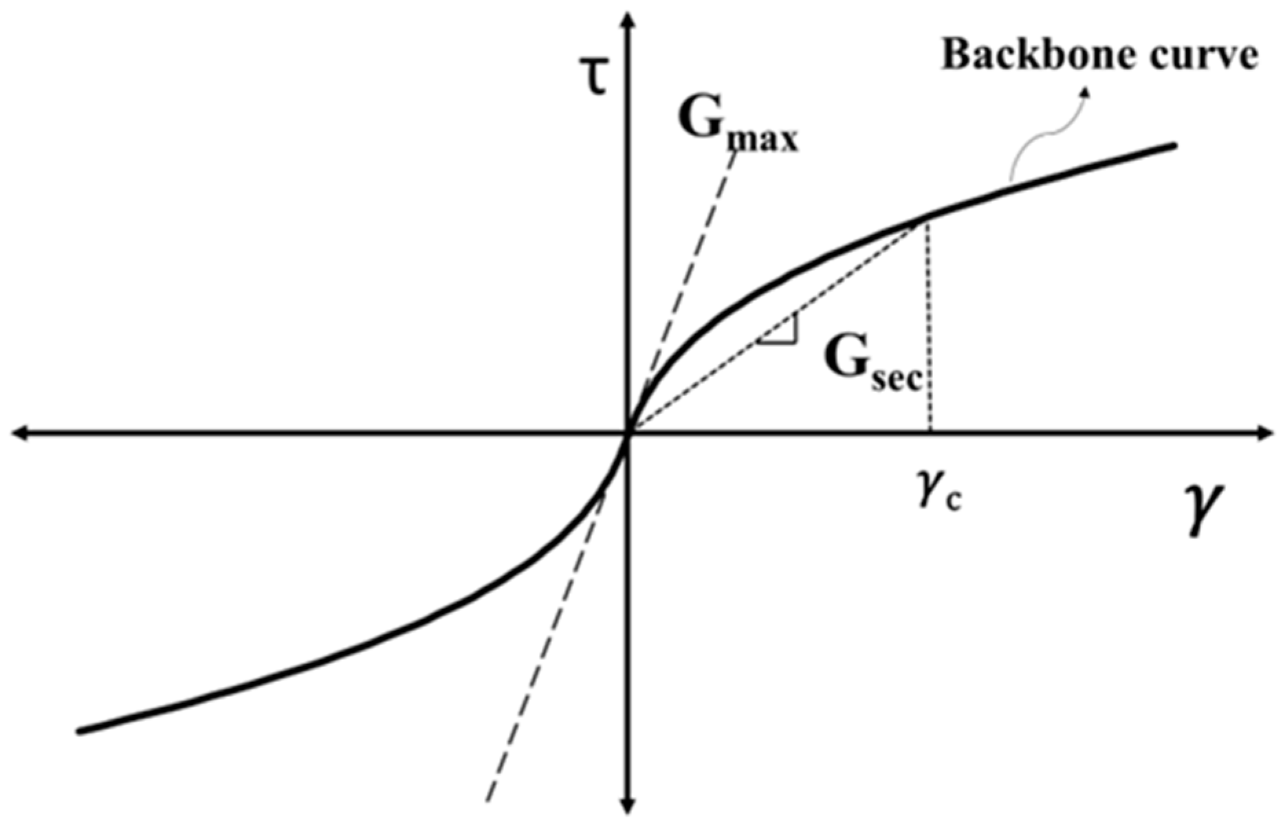
Figure 3.
The secant shear modulus and damping ratio. (a) A hysteresis loop and the calculation of the secant shear modulus and viscous damping ratio. (b) Increase in damping ratio with strain rate.
Figure 3.
The secant shear modulus and damping ratio. (a) A hysteresis loop and the calculation of the secant shear modulus and viscous damping ratio. (b) Increase in damping ratio with strain rate.
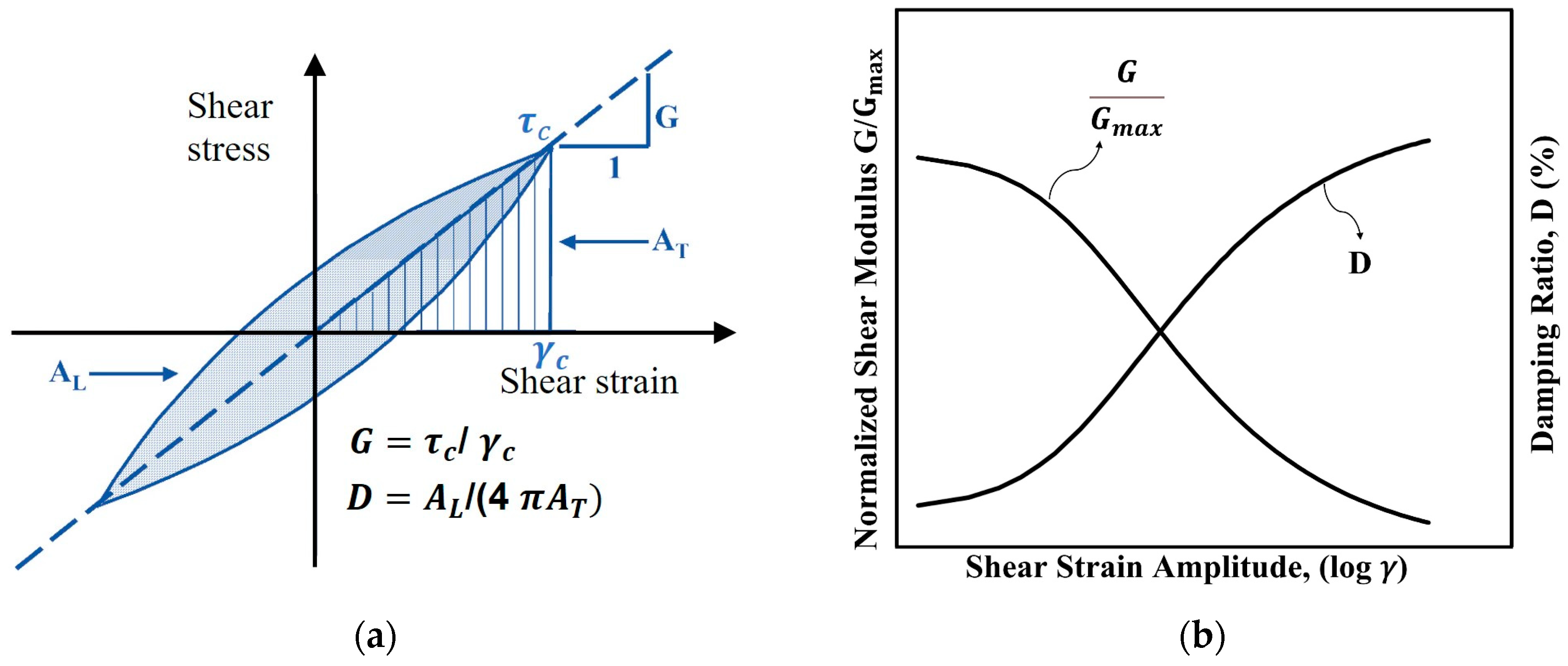
Figure 4.
The decaying response in the RC test.
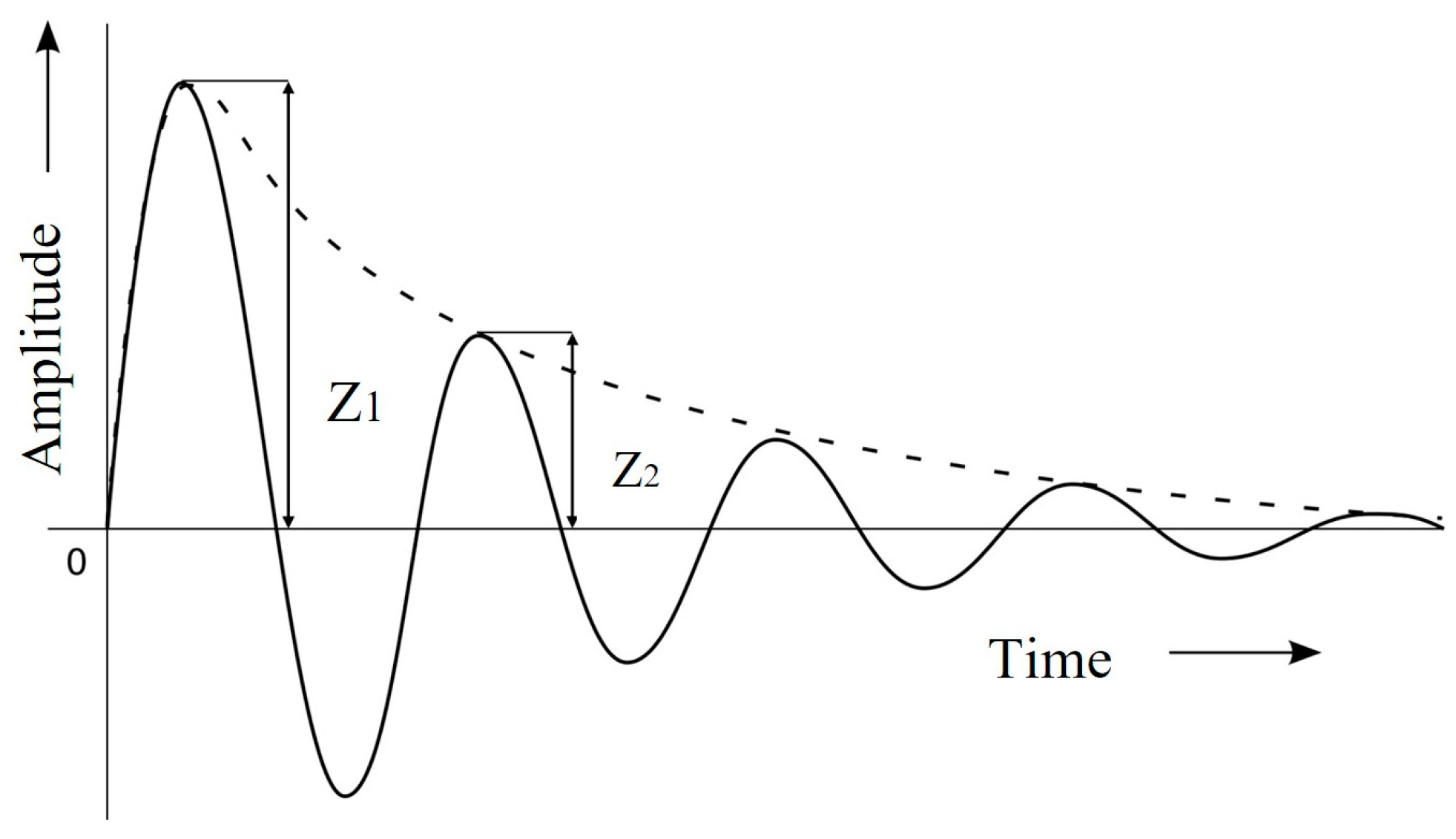
Figure 5.
Resonance frequency in RC test.
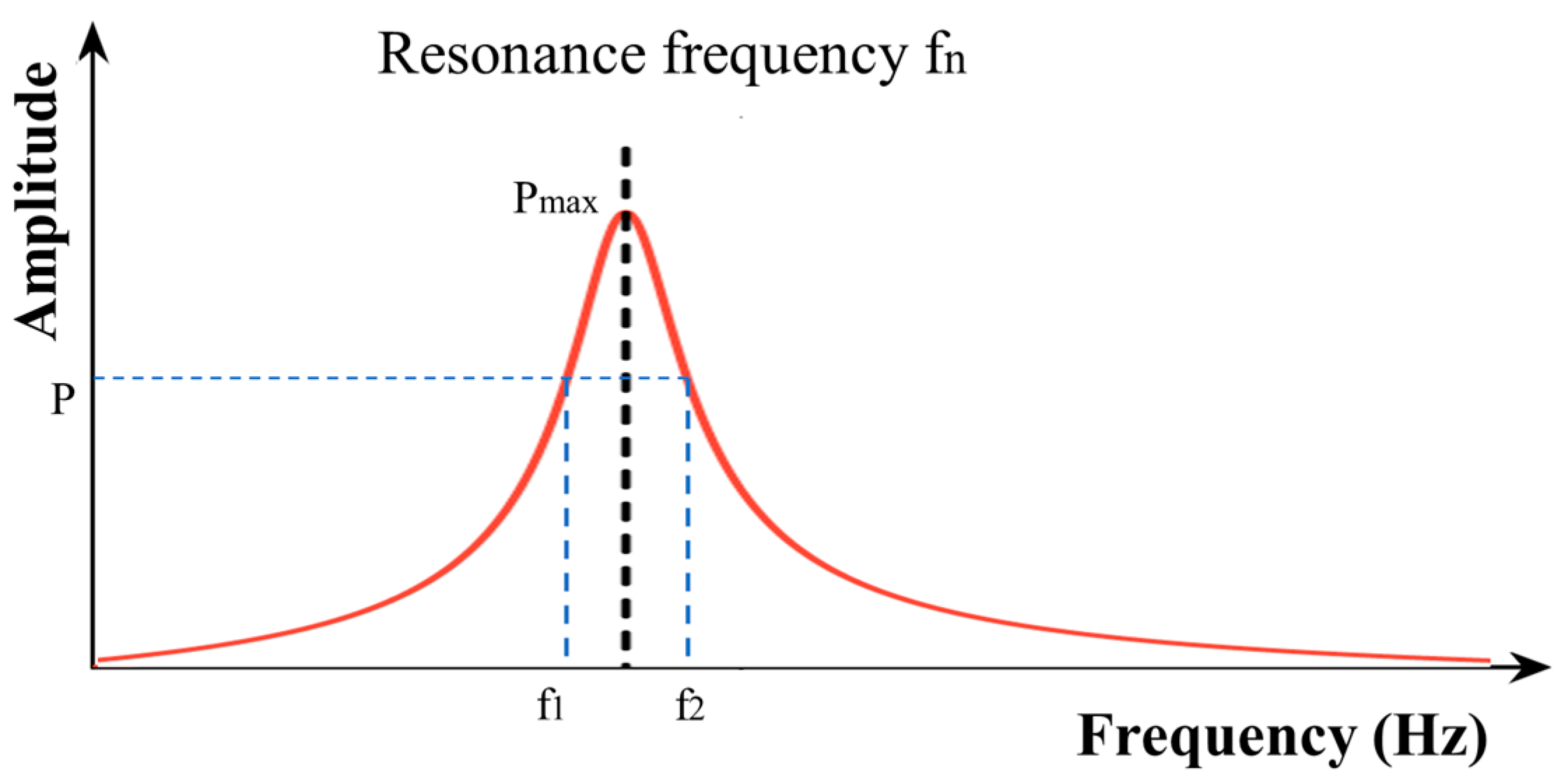
Figure 6.
Diagram of the concept for torsional strain in a fixed-free hollow cylinder specimen.

Figure 7.
Shear wave velocity increase with confinement time after Stokoe and Richart [53] (open access).
Figure 7.
Shear wave velocity increase with confinement time after Stokoe and Richart [53] (open access).
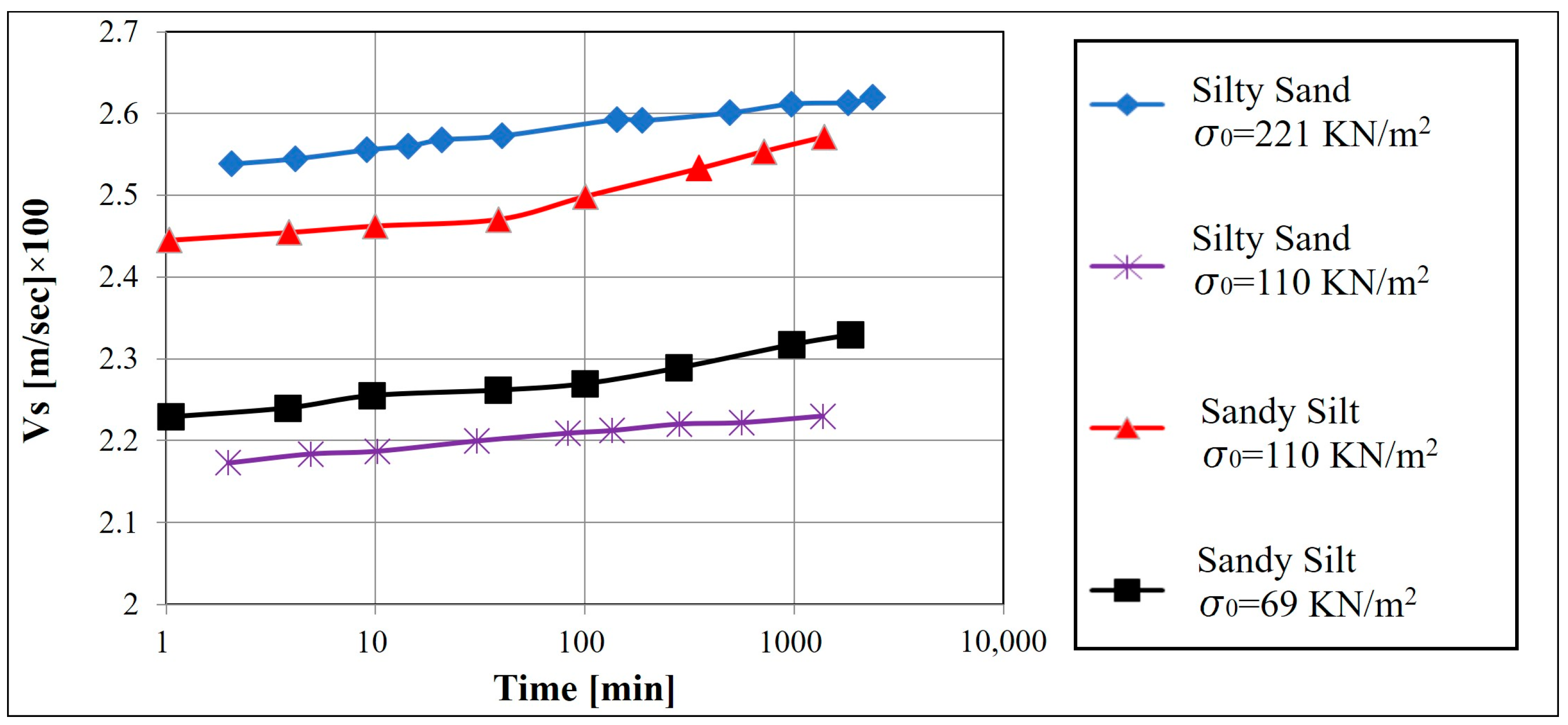
Figure 8.
Effect of pre-vibration on Gmax for a confining stress of 100 KPa, after Yang et al. [63] (permission from [ASCE].
Figure 8.
Effect of pre-vibration on Gmax for a confining stress of 100 KPa, after Yang et al. [63] (permission from [ASCE].
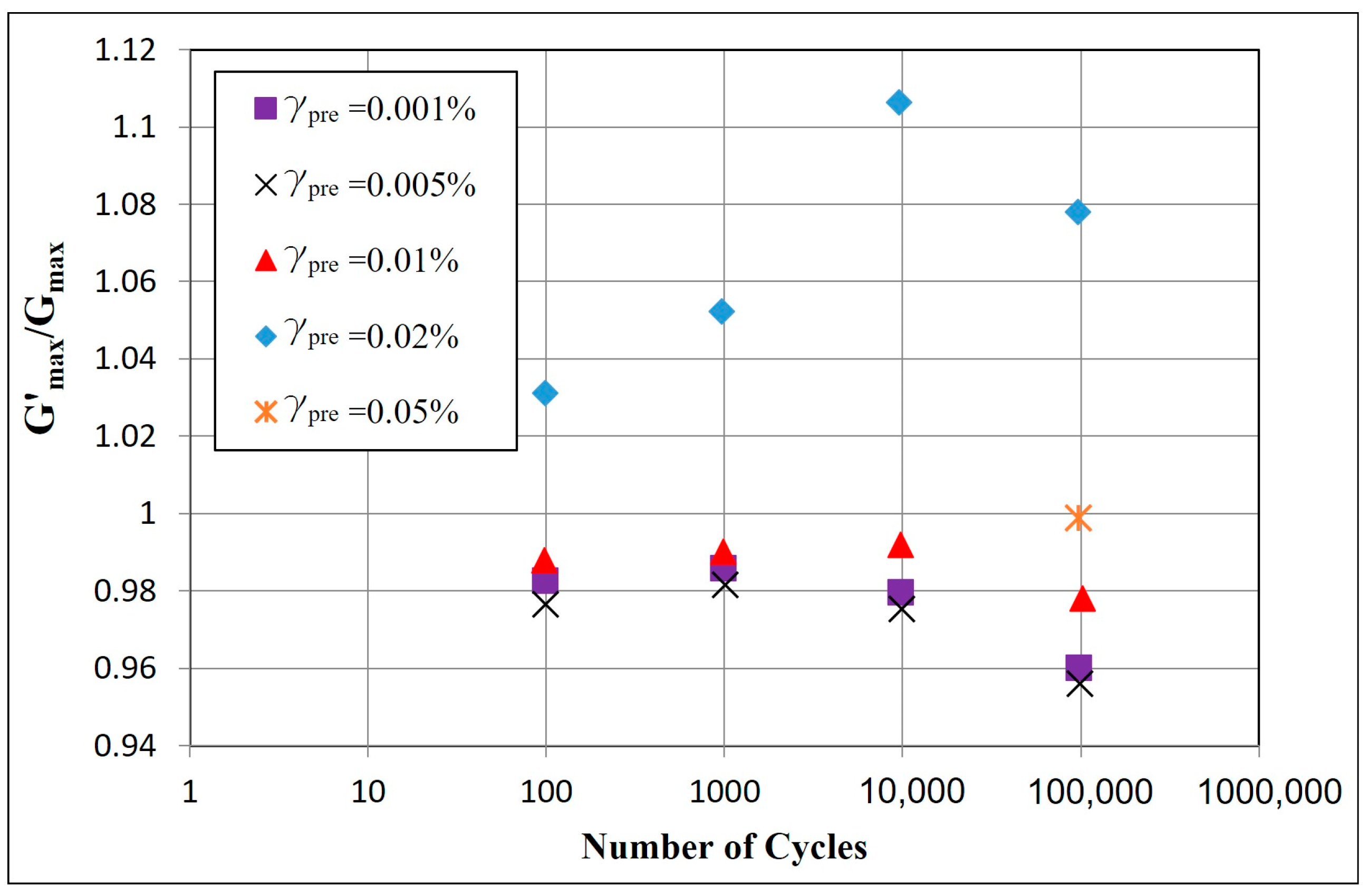
Figure 9.
Coefficients for Equation (26) after Oztoprak and Bolton [79] (permission from [ICE]).
Figure 9.
Coefficients for Equation (26) after Oztoprak and Bolton [79] (permission from [ICE]).

Figure 10.
Comparison of measured shear wave velocity values [88] (reprinted, open access CC BY).
Figure 10.
Comparison of measured shear wave velocity values [88] (reprinted, open access CC BY).
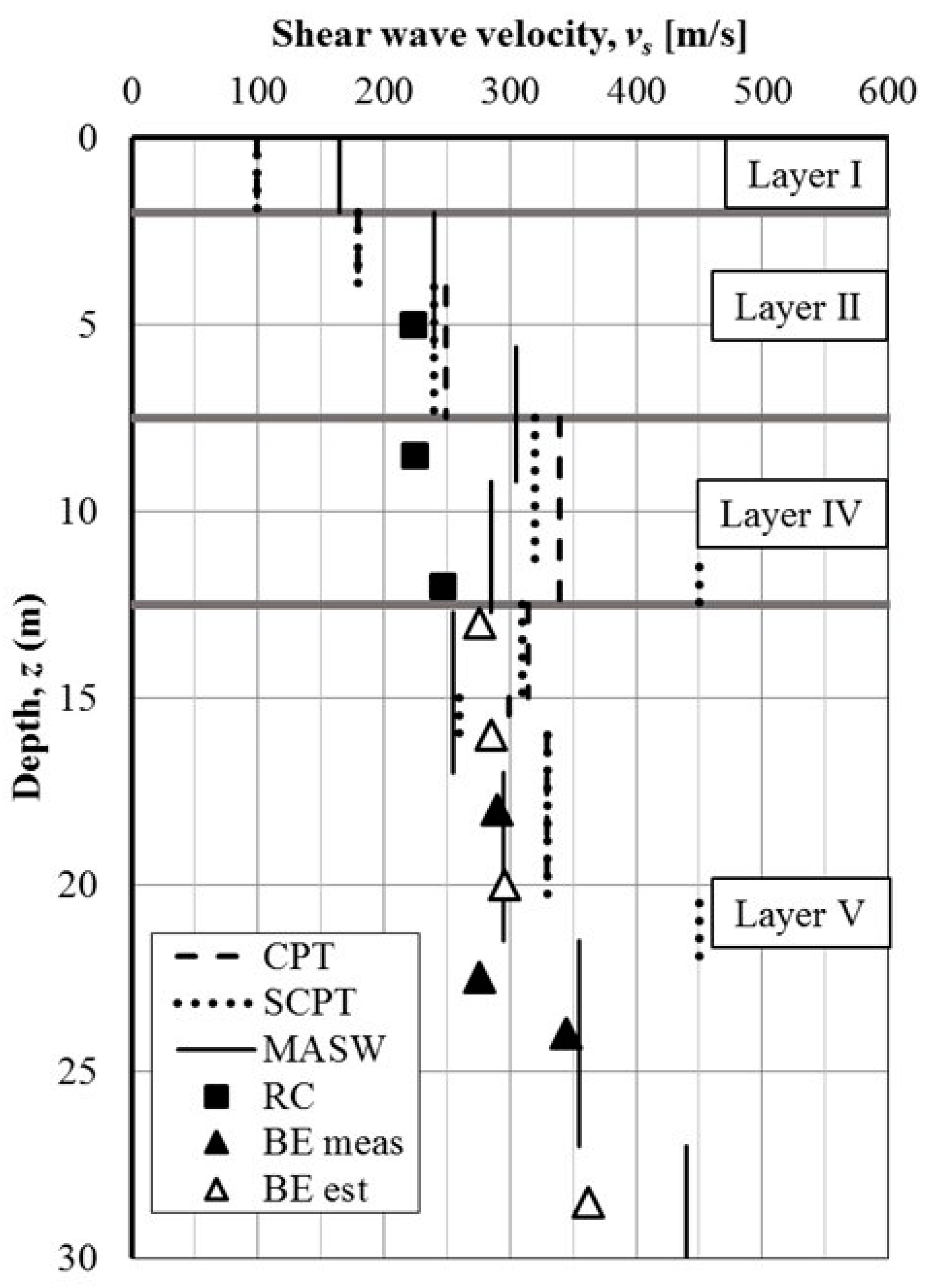
Figure 11.
Temperature effect with the measured values (symbols) and fitting curves (lines) [92] (reprinted, open access CC BY). (a) Modulus ratio. (b) Damping ratio.
Figure 11.
Temperature effect with the measured values (symbols) and fitting curves (lines) [92] (reprinted, open access CC BY). (a) Modulus ratio. (b) Damping ratio.

Figure 12.
Effect of crumb rubber on the dynamic properties of sand at a strain amplitude of 0.02% based on Das and Bhowmik [93] (permission from [ASCE]). (a) Effect on the shear modulus degradation curve. (b) Effect on the damping ratio.
Figure 12.
Effect of crumb rubber on the dynamic properties of sand at a strain amplitude of 0.02% based on Das and Bhowmik [93] (permission from [ASCE]). (a) Effect on the shear modulus degradation curve. (b) Effect on the damping ratio.

Figure 13.
Steel slag and cement additives for sand (150 kPa-7 days) [95] (reprinted with permission from [Elsevier]). (a) Effect on the shear modulus. (b) Effect on the damping ratio.
Figure 13.
Steel slag and cement additives for sand (150 kPa-7 days) [95] (reprinted with permission from [Elsevier]). (a) Effect on the shear modulus. (b) Effect on the damping ratio.
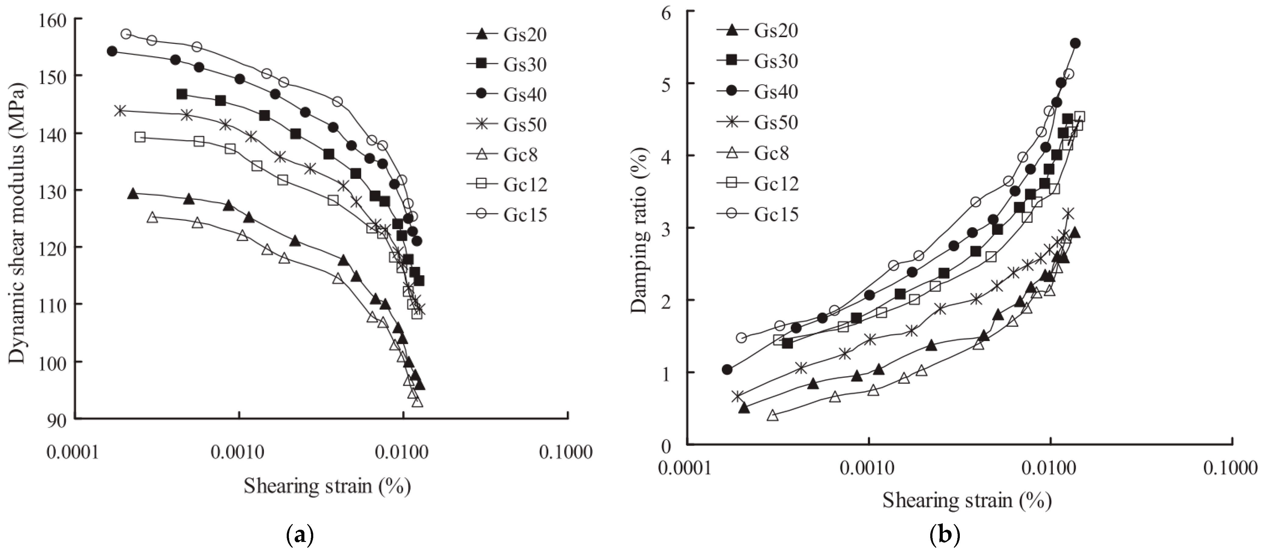
Figure 14.
Improvement in the shear of clean sands due to grouting [96] (reprinted with permission from [Elsevier]).
Figure 14.
Improvement in the shear of clean sands due to grouting [96] (reprinted with permission from [Elsevier]).
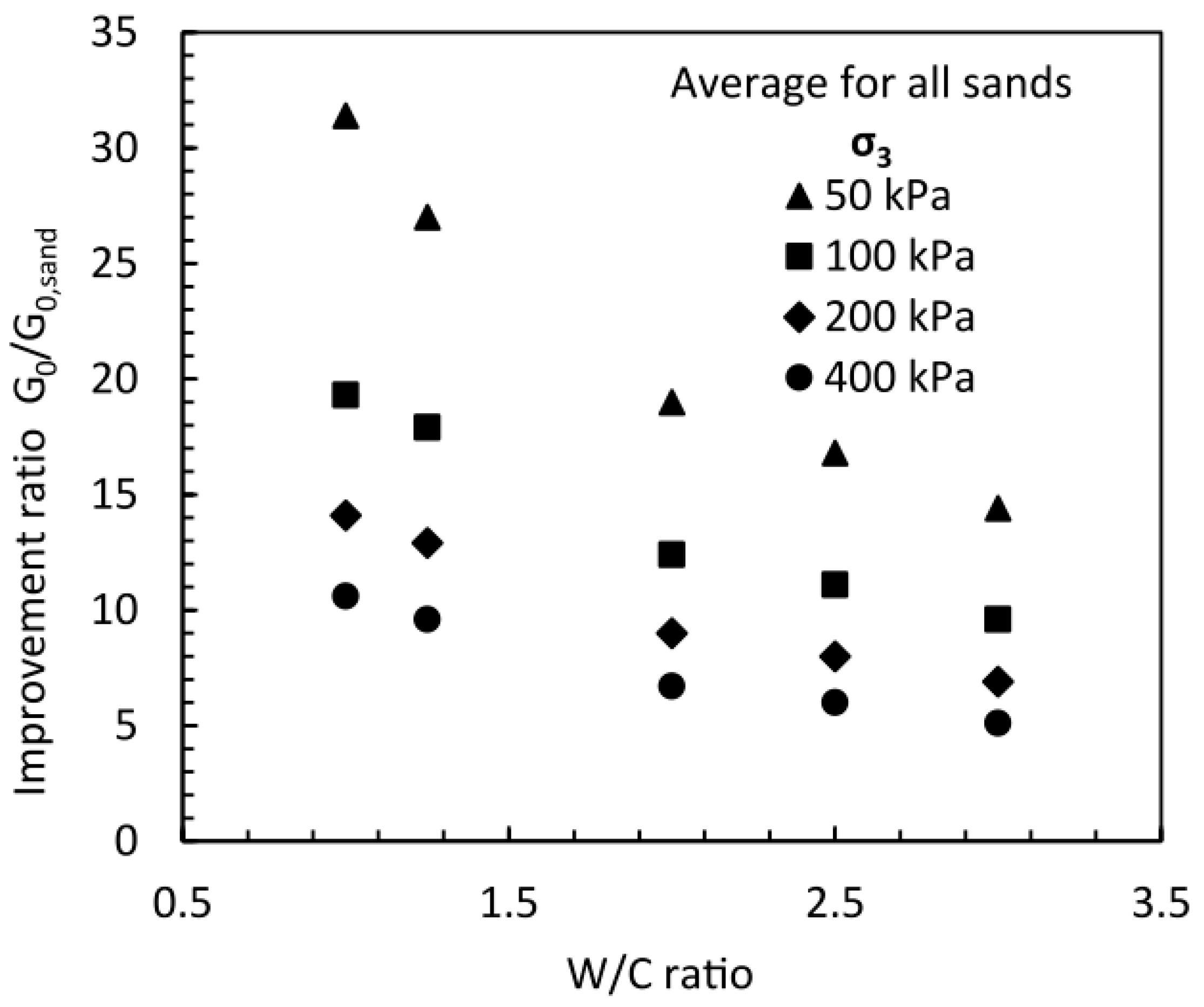
Figure 15.
Dynamic properties of rubber-sand mixture with varying rubber content [97] (reprinted with permission from [Elsevier]). (a) Dynamic shear modulus properties. (b) Damping ratio properties.
Figure 15.
Dynamic properties of rubber-sand mixture with varying rubber content [97] (reprinted with permission from [Elsevier]). (a) Dynamic shear modulus properties. (b) Damping ratio properties.
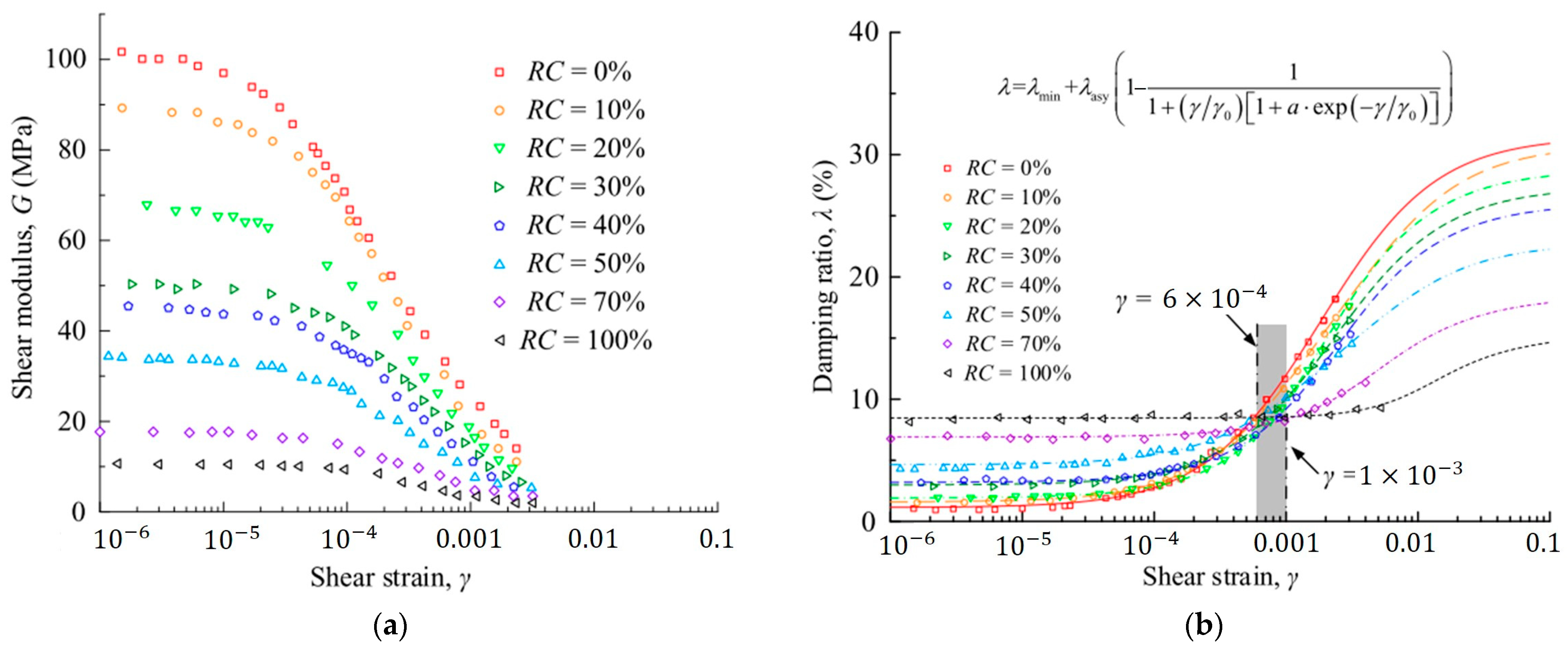
Figure 16.
Masing criteria.
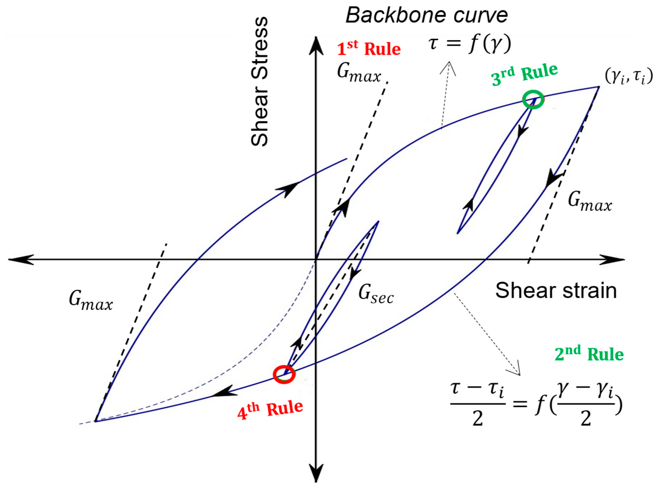
Figure 17.
Hysteresis loops according to the extended Masing rules using the Ramberg-Osgood model after Pyke [99] (permission from [ASCE]). (a) Symmetric. (b) Irregular loading with Pyke’s discussion.
Figure 17.
Hysteresis loops according to the extended Masing rules using the Ramberg-Osgood model after Pyke [99] (permission from [ASCE]). (a) Symmetric. (b) Irregular loading with Pyke’s discussion.
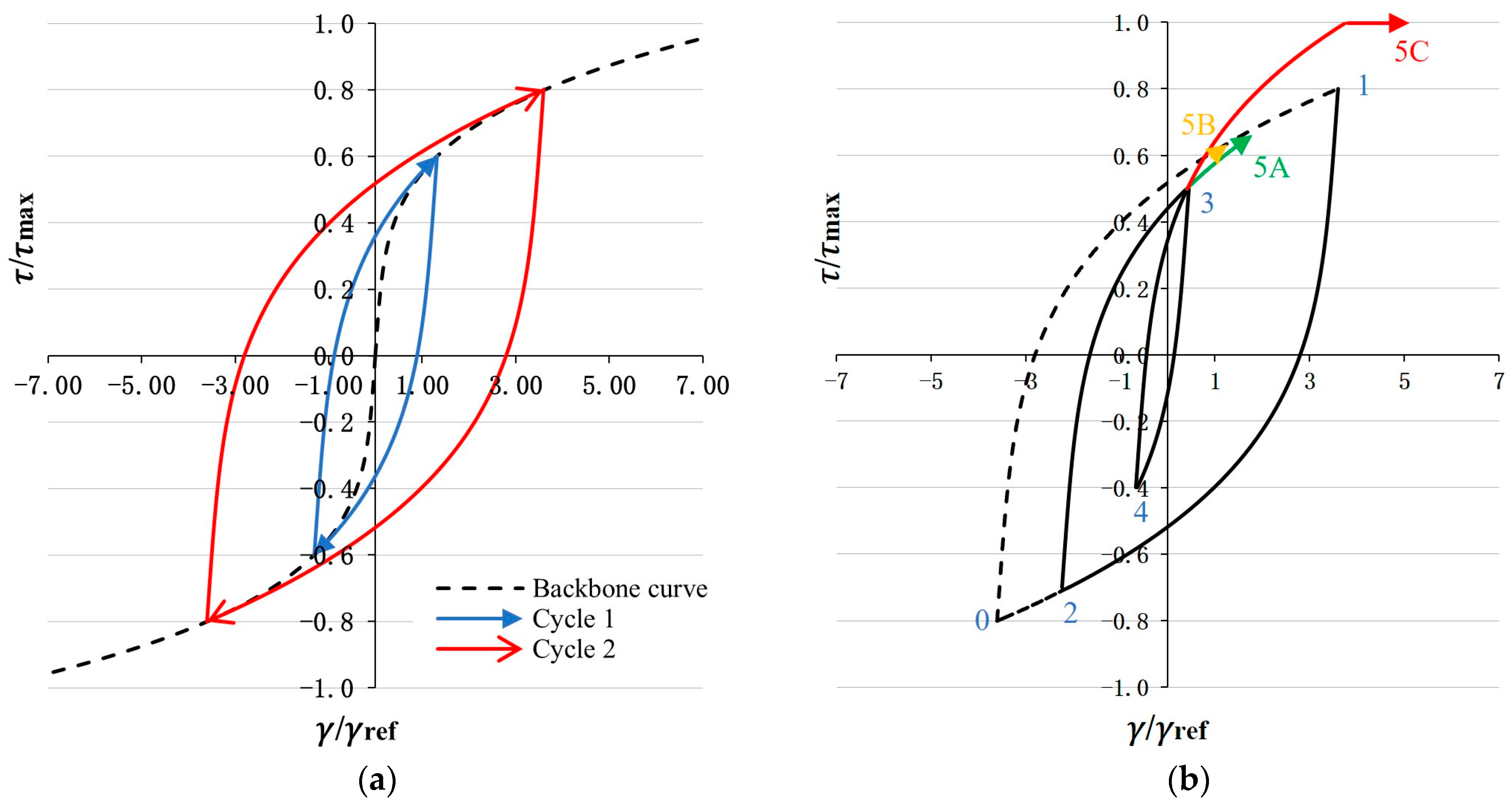
Figure 18.
Normalized secant and tangent modulus vs. strain obtained using the Ramberg-Osgood model.
Figure 18.
Normalized secant and tangent modulus vs. strain obtained using the Ramberg-Osgood model.
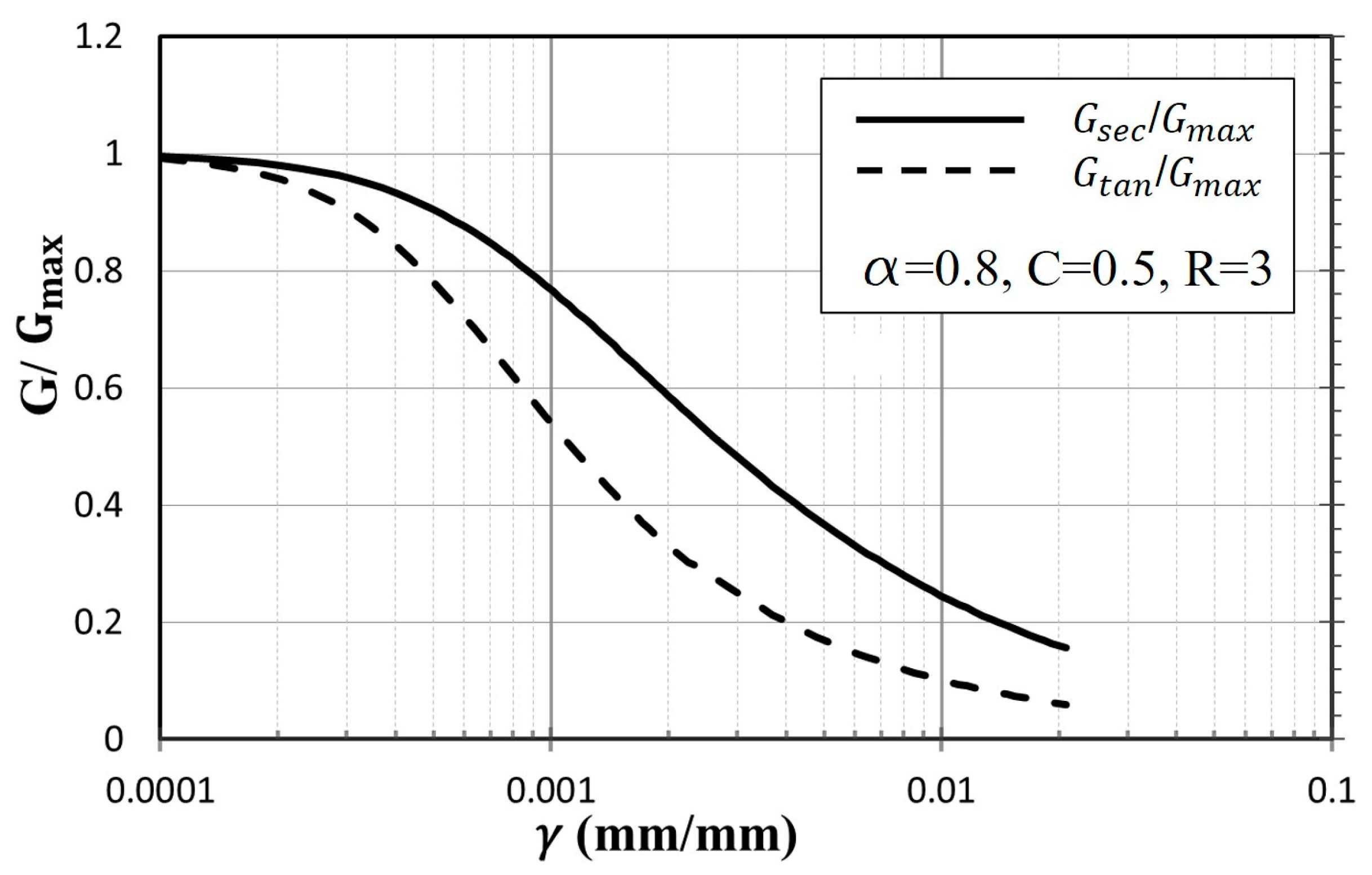
Figure 19.
Mohr diagram for maximum shear stress.
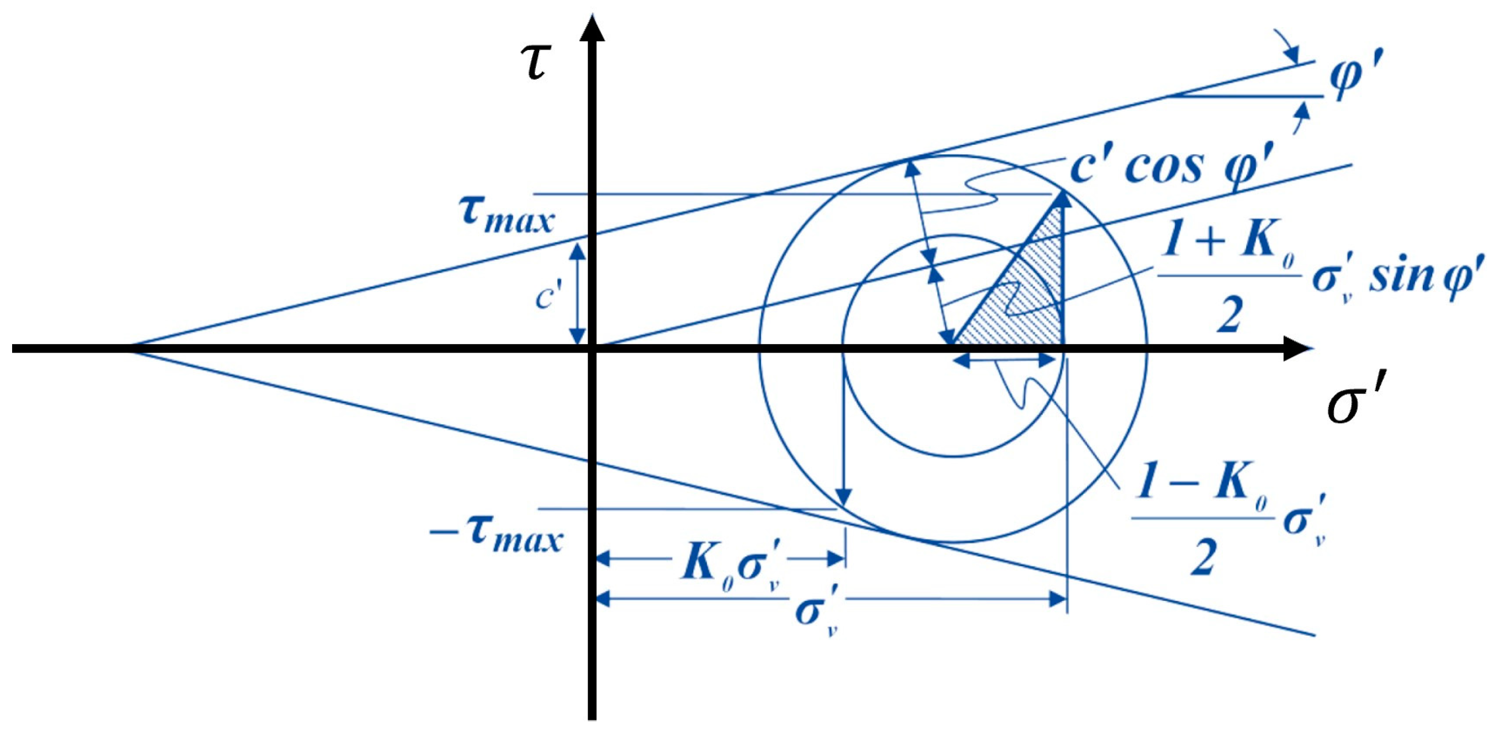
Figure 20.
Integration element for half a loop in RO model.
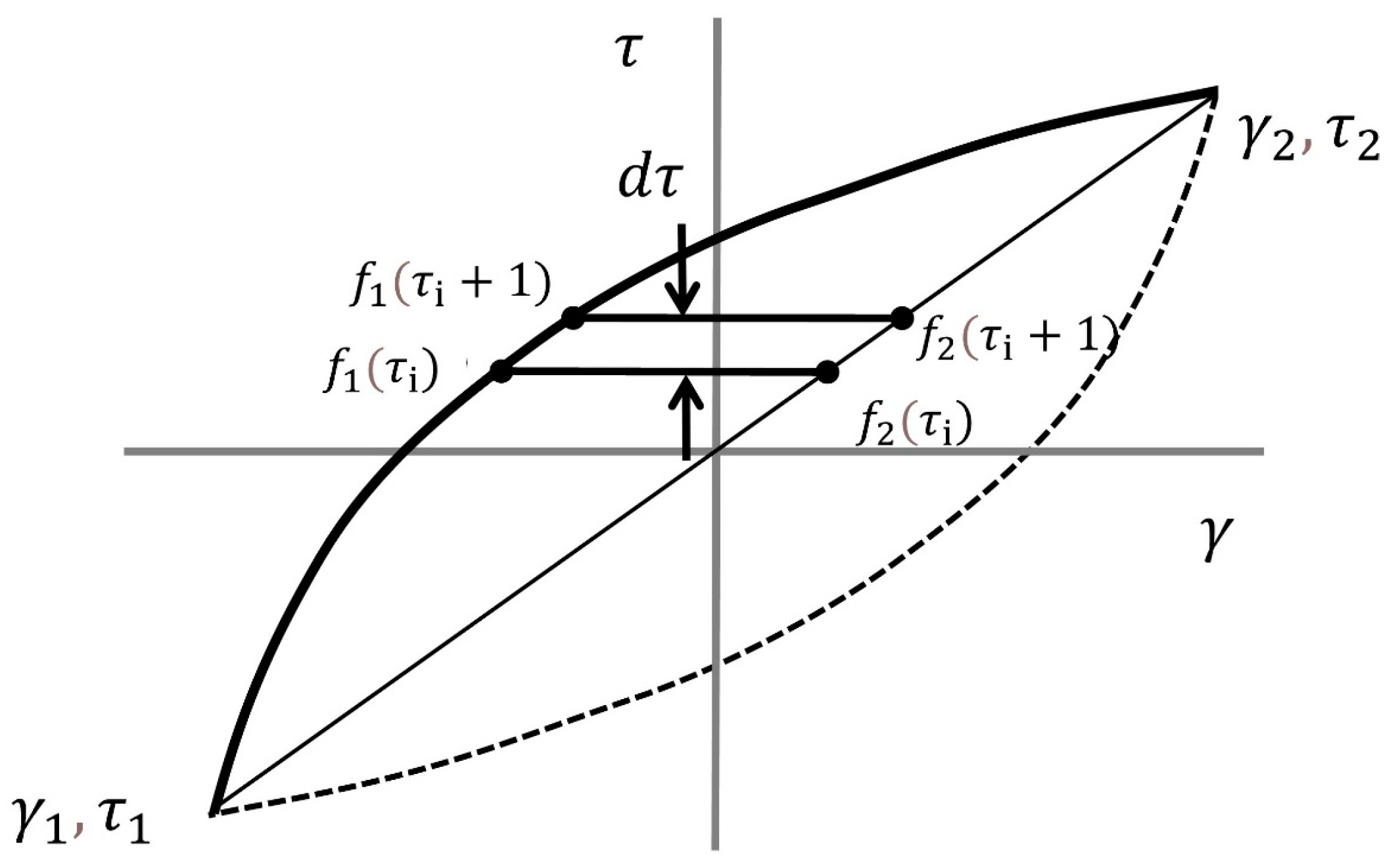
Figure 21.
The hyperbolic model proposed by Hardin and Drnevich (1972) [40] (permission from [ASCE]). (a) Hyperbolic soil model equation. (b) The deviation from a hyperbole, depending on soil type.
Figure 21.
The hyperbolic model proposed by Hardin and Drnevich (1972) [40] (permission from [ASCE]). (a) Hyperbolic soil model equation. (b) The deviation from a hyperbole, depending on soil type.

Figure 22.
Normalized modulus reduction curve using a modified hyperbolic model for .
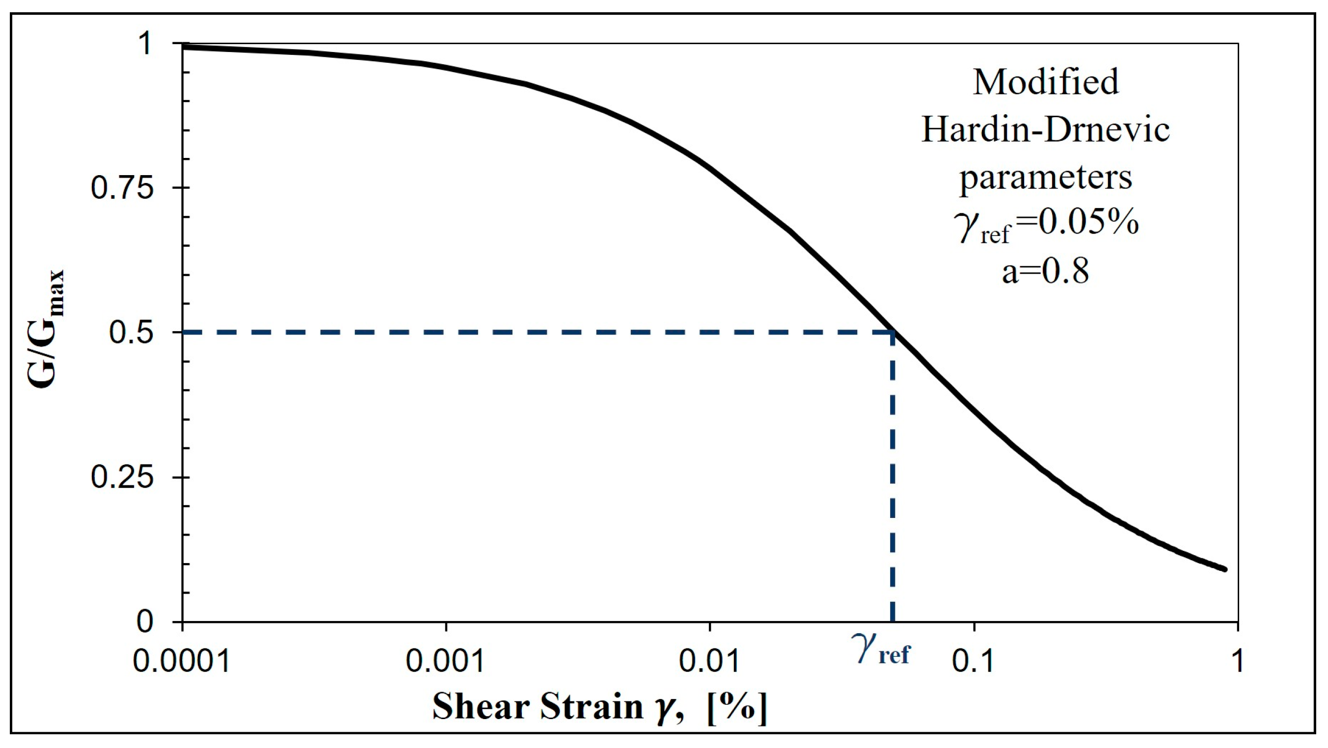
Figure 23.
Comparison between the RO and HD model in Midas GTS NX [46] (open access CC BY). (a) Fit of RO model with the TOSS test results. (b) Fit of HD model with the TOSS test results.
Figure 23.
Comparison between the RO and HD model in Midas GTS NX [46] (open access CC BY). (a) Fit of RO model with the TOSS test results. (b) Fit of HD model with the TOSS test results.
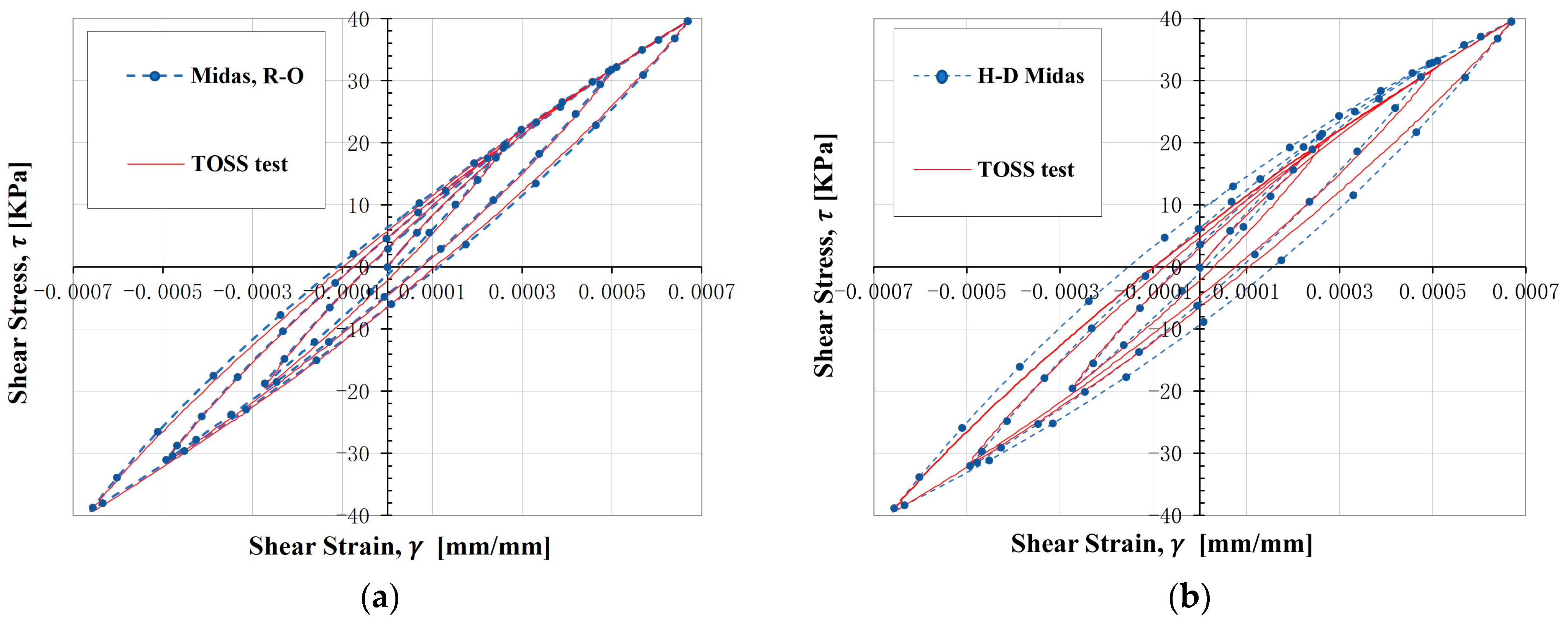
Figure 24.
Numerical study of random material properties within a soil specimen [111] (reprinted, open access CC BY). (a) Mesh with rigid links attached and applied twist (ϕz). (b) Workflow of the analysis.
Figure 24.
Numerical study of random material properties within a soil specimen [111] (reprinted, open access CC BY). (a) Mesh with rigid links attached and applied twist (ϕz). (b) Workflow of the analysis.

Table 1.
Features, advantages, and disadvantages of RC-TOSS testing system.
| Feature | Advantage | Disadvantage |
|---|---|---|
| RC (accelerometer) | Very accurate and repeatable readings over a broad strain range. | Test must be dynamically excited |
| TOSS (proximitors) | Accurate over a slightly smaller strain range. Cyclic, cyclic with static offset, irregular loading programmed in the control software | Proximitor response is nonlinear and requires careful calibration, set-up, and computation during the test. |
| RC-TOSS (hollow cylinder specimen | More uniform strains in the specimen. Highly tolerant of voids/inclusions (gravel, organics). | Two membranes (inner, outer) and a more complex system to construct specimens. Dry pluviation, vibrating, or hand trimming (cohesive) in special mold requires ~2–3 h prep time. |
| RC-TOSS (coil-magnet loading) | RC and TOSS tests are performed on the same specimen in multiple stages. | Limit to a maximum torque of about 55 N-m |
Table 3.
Parameters of the frozen silt modulus ratio and damping ratio curves at different temperatures [92] (reprinted, open access CC BY).
Table 3.
Parameters of the frozen silt modulus ratio and damping ratio curves at different temperatures [92] (reprinted, open access CC BY).
| Temperature [°C] | Gmax [MPa] | Dmax [−] | N [−] | |
|---|---|---|---|---|
| −15 | 1539.2 | 6.312 × 10⁻⁵ | 0.073 | 0.42 |
| −10 | 1467.4 | 6.670 × 10⁻⁵ | 0.078 | 0.36 |
| −5 | 1341.8 | 7.520 × 10⁻⁵ | 0.106 | 0.44 |
| −3 | 1238.4 | 9.354 × 10⁻⁵ | 0.116 | 0.36 |
| Room temperature (15 °C to 25 °C) | 64.2 | 6.602 × 10⁻⁴ | 0.183 | 0.60 |
Disclaimer/Publisher’s Note: The statements, opinions and data contained in all publications are solely those of the individual author(s) and contributor(s) and not of MDPI and/or the editor(s). MDPI and/or the editor(s) disclaim responsibility for any injury to people or property resulting from any ideas, methods, instructions or products referred to in the content. |
© 2023 by the authors. Licensee MDPI, Basel, Switzerland. This article is an open access article distributed under the terms and conditions of the Creative Commons Attribution (CC BY) license (https://creativecommons.org/licenses/by/4.0/).
Share and Cite
MDPI and ACS Style
Ahmad, M.; Ray, R. The Dynamic Properties of Sand under Torsion: A Literature Review. Geotechnics 2023, 3, 480-514. https://doi.org/10.3390/geotechnics3020027
AMA Style
Ahmad M, Ray R. The Dynamic Properties of Sand under Torsion: A Literature Review. Geotechnics. 2023; 3(2):480-514. https://doi.org/10.3390/geotechnics3020027
Chicago/Turabian StyleAhmad, Majd, and Richard Ray. 2023. "The Dynamic Properties of Sand under Torsion: A Literature Review" Geotechnics 3, no. 2: 480-514. https://doi.org/10.3390/geotechnics3020027