Mutation Trajectory of Omicron SARS-CoV-2 Virus, Measured by Principal Component Analysis

Abstract

Since 2019, the SARS-CoV-2 virus has caused a global pandemic, resulting in widespread infections and ongoing mutations. Analyzing these mutations is essential for predicting future impacts. Unlike influenza mutations, SARS-CoV-2 mutations displayed distinct selective patterns that were concentrated in the spike protein and small ORFs. In contrast to the gradual accumulation seen in influenza mutations, SARS-CoV-2 mutations lead to the abrupt emergence of new variants and subsequent outbreaks. This phenomenon may be attributed to their targeted cellular substances; unlike the influenza virus, which has mutated to evade acquired immunity, SARS-CoV-2 appeared to mutate to target individuals who have not been previously infected. The Omicron variant, which emerged in late 2021, demonstrates significant mutations that set it apart from previous variants. The rapid mutation rate of SARS-CoV-2 has now reached a level comparable to 30 years of influenza variation. The most recent variant, JN.1, exhibits a discernible trajectory of change distinct from previous Omicron variants.

1. Introduction

COVID-19, caused by the SARS-CoV-2 virus, is an unprecedented infectious disease responsible for numerous cases and fatalities worldwide [1]. The virus has undergone successive mutations [2,3], and understanding these mutations is crucial for predicting its future behavior. The spike protein of this virus binding to the human ACE2 protein is a crucial early event in infection. Therefore, mutations in this virus are being investigated primarily around this spike protein [4]. These mutations can lead to markedly reduced serum neutralization [5,6,7] and/or stronger binding to ACE2 [8,9,10,11]. Given that many independent mutations often converge in evolution [12,13,14], they are believed to enhance adaptation to humans. However, considering the virus’s entire length of 30,000 bases, mutations are even more diverse, making it essential to study the entire genome to understand viral evolution.

The purpose of the study is twofold. Firstly, to understand the characteristics of the Omicron variant and how it has evolved. Previously, the WHO has distinguished variants, particularly those with high transmissibility and widespread infections, by assigning them Greek letters starting with Alpha [15]. However, the Omicron variant, which emerged at the end of 2021, has proven to be more transmissible than any previous variant, persisting and dominating the virus’s brief history for about half of its duration.

Secondly, to compare the changes in the SARS-CoV-2 virus with those of influenza H1N1 virus. Influenza viruses, which are similarly highly transmissible and cause annual outbreaks, are often equated with COVID-19. However, is this a valid comparison? Or might these have entirely different natures? Those were investigated by using principal component analysis (PCA) [16].

PCA offers several compelling advantages over more prevalent clustering methods. Its primary strength lies in its ability to provide a comprehensive overview. While clusters primarily indicate the proximity between adjacent samples, PCA offers a holistic perspective, revealing the inter-group distances and the degree of divergence exhibited by new variants. Furthermore, PCA elucidates sequential differences between individual variants through PC_item, a level of detail often obscured in clustering analyses. Importantly, PCA results are highly reproducible across calculations, which ensures consistency in the outcomes. Additionally, PCA facilitates the straightforward positioning of new samples along the identified axes, a task that necessitates the recalibration of clustering methods for each new sample. This attribute proves advantageous for classification tasks.

2. Materials and Methods

2.1. PCA

The sequencing arrays were analyzed using PCA. Multivariate data, such as aligned sequencing arrays, can be marked in the form of a matrix. There are rows corresponding to each sample and columns recording each item measured. This can be thought of as each sample having a unique position in the number of dimensions equal to the number of items, or each item having a unique position in the number of dimensions equal to the number of samples. Each of these dimensions has its own axis, and each axis is orthogonal.

In the case of sequencing data, the dimensionality can be extremely high. For aligned sequences, each item represents the type of base (or amino acid) present at each position. The number of samples is often large, and the number of bases can also be substantial. In the case of COVID, for instance, there are approximately 300,000 bases. Regardless, the dimensionality becomes incredibly large, making it difficult for us to comprehend. Therefore, it is desirable to reduce the dimensionality. PCA is a method designed for this purpose. Samples and items are not necessarily independent; they may exhibit similar trends. By grouping these together, the dimensionality can be reduced. These similar trends can be represented by a single line that shows a direction within the matrix. PCA rotates the entire matrix so that this line aligns with one of the orthogonal axes. By repeating this process, it becomes possible to describe all of the data with far fewer axes than in the original ones. In particular, axes that many samples or items align with tend to carry more information.

The calculation is executed using a matrix calculation called singular value decomposition (SVD), represented as M = UDV*, where V* is the conjugate transpose of V: transposing V and applying complex conjugation to each entry. Here, M is any matrix of which each column represents a single item of sample. A row represents a sample. U and V are unitary matrices representing the direction associated with the sample and item, respectively, and D is a diagonal matrix indicating distance. As a property of the unitary matrix, U and V are square matrices. Moreover, U* U = UU* = I, meaning the inner product with its own adjugate matrix (transpose matrix) becomes the identity matrix. This has two meanings. Firstly, all rows and columns of these have a squared sum of one. This means that all row vectors and column vectors decomposed from the unitary matrix have a Euclidean distance of one. Hence, the matrix only records direction and does not record distance; by taking the inner product with this and a matrix, the matrix can simply be rotated. Secondly, the inner products of column vectors or row vectors all become zero (except for oneself). This indicates that all vectors are independent and orthogonal to each other.

A principal component (PC) is estimated by assigning distance in a specific direction. Two types of PCs are given. One is the sample PC, which is mainly used in this article. It shows the things that are similar between the samples and those that are significantly different. The other is the item PC. The sample PC and item PC are calculated as follows:

PC_sample = MV = UD

PC_item = M* U = VD

The distances in D are sorted in order of size. Therefore, within each column the PCs are displayed in order of size. These are called PC1, PC2, …, respectively. Each PC is aligned in one independent direction. From this D, the contribution of each PC can be measured. Specifically, it is diag(D)/ΣD, where diag(D) is the diagonal component of D.

Mutations are categorized across multiple axes, with the significance of each axis intensifying as a substantial number of mutations accumulate. This significance is quantified by the extent to which the axis encompasses the mutations, termed as contribution. Usually, PC_sample is normalized by the number of items and PC_item by the number of samples to facilitate the comparison with different sizes [16]. This is because D varies depending on the number of items and samples, and this measure is to eliminate such effects. This allows for comparisons beyond calculations. However, in this study, PC_sample was not normalized. Therefore, the numbers represent the changed amino acids as they are.

As is evident from PC_sample = UD, PC_item = VD, and M = UDV, M can be reproduced from the two types of PCs. This means that PCA is a method that does not lose data information. This is significantly different from, for example, cluster analysis, which is calculated after making a distance matrix, which does not have information on items. On the other hand, in PCA, when a certain PC separates samples, the items that were involved are displayed in the PC_item of the same rank.

SVD is a highly objective calculation method with no options to choose from. Therefore, the same values can be obtained no matter who performs it, resulting in high reproducibility. This is different from cluster analysis, which has various options for defining and calculating distances.

2.2. PCA for Sequencing Data

In the case of sequencing data, items are bases or amino acids, so they cannot be calculated. To compensate for this, a Boolean conversion is performed [16]. In other words, items are converted to zero and one. This does not result in data loss, as only the method of marking changes, and there is no data loss. One of the few options in PCA is where to position the center of rotation. Here, the average sequence of all data is used as the center. We used M centered at one, subtracted by the average sample. When examining types of variation, it is conceivable to use the sample related to the before and after of the variation as the center. The computations were performed using R [17], employing the same PCA methodology and R-code as those outlined in a previous publication [16]. In addition, the R code is freely available in github as a compressed form at https://github.com/TomokazuKonishi/direct-PCA-for-sequences (accessed on 7 April 2024).

2.3. Data Curation

Sequence data were obtained from GISAID [18], with weekly systematic selection to minimize country overlap. Alignment was performed using the DECIPHER function [19]. For the PCA of the S proteins, the axes were found by sorting the collection dates and arranging them by month, sampling 30 for each month, to avoid bias due to time of year. For the nucleic acid sequences, axes created previously, when the Omicron variant had just emerged, were used [2]. The PC was computed by fitting these axes to individual data points. Detailed calculations, including PC_sample and PC_item, are provided in the Supplementary Materials. Protein analyses were conducted using translated segments, with influenza virus data sourced from prior publications [16]. R codes for protein analyses are included in this article.

PCA does have a limitation: mutations not aligned with the axes are not visible, even though a higher PC may show many mutations, and this may not be the case for all mutations. Therefore, it is essential to consider and examine mutations down to lower PCs. Supplements are available for this purpose. As the number of figures in the Supplement is inevitably very large, they are provided in HTML format. For ease of viewing, most of the figures are hidden behind the icons. To view them, or to enlarge them, click on the small diagrams provided as icons. In particular, 3D structures cannot be shown in detail in the printed media; see the diagrams that can be moved in HTML.

2.4. 3 D Structure of Proteins

For the 3D model of the spike protein, we selected 7DWZ [20] from the RCSB Protein Data Bank [21] due to its closest sequence resemblance and the absence of a His-tag at the C-terminus [22]. Using ATOM data from this structure, we extracted the α-carbon position of each amino acid and connected them with lines using the rgl function in R [23]. Amino acids corresponding to mutations were identified based on significant changes (>0.005) by selecting the axis with the greatest alteration for each from the PC_sample and determining the standard deviation (SD) from the PC_item values along the same axis. All mutations exceeding a large SD across all sequences (>0.036) were included. These thresholds were identified as inflection points in the normal probability plot.

3. Results

3.1. Mutations Observed from Nucleotide Sequence

How has SARS-CoV-2 mutated? Previous variants up to Omicron diverged into three lineages [24]. With the exception of the earliest ones, the trajectory was predominantly unidirectional. However, the emergence of the Omicron variant resulted from a significant mutation in a direction distinct from that of its predecessors (see Figure 1A). Previous mutations are nearly linearly represented in PC2, with Delta appearing positive and Lambda the most negative. In contrast, Omicron is situated at an almost perpendicular deviation from the trajectory, followed by variants delineated by PC1. A higher level of PC indicates a greater number of mutations in the direction. The perpendicular deviation is attributed to the emergence of mutations completely unrelated to those observed in prior variants.

One of the advantages of PCA is that it allows us to compare transitions in data across different categories, such as time, for example. This is easy to comprehend if we consider doing the same thing with clustering. PC1, for instance, revealed the most significant relationships among the numerous variants, including older variants such as Alpha to Delta and the more recent JN.1. (for temporal changes in other PCs, refer to Figure S3 by clicking the iconic figure). Figure 1B illustrates this temporal progression.

Examination of PC1 in chronological order revealed the sudden emergence of the BA.1 variant (Figure 1B). Ideally, such an event should result from a gradual accumulation of mutations; however, due to mutations occurring in unsequenced regions, possibly in an African country, intermediate stages were unrecorded [2]. Following the date indicated by the dashed vertical line (1 December 2021), the prevalence of preceding variants swiftly declined, giving way to the dominance of BA.1. Some of these variants feature insertions in the spike protein (Spike ins214EPE). Subsequently, the BA.1 outbreak also subsided, making room for other Omicron variants (Figure 1B). Notably, some of the latest JN.1 variants exhibit insertions (Spike ins16MPLF). Although deletions are commonly observed in the short history of SARS-CoV-2 variations, insertions are relatively rare. It is not known which mutations preceded JN.1, but this is closer to earlier variants than the Omicrons (Figure 1A). As is clear in Figure 1B, many of the sequence features exhibited by BA.1 and shared among Omicrons have been lost from JN.1.

A significant disparity existed between the mutational patterns observed for SARS-CoV-2 and influenza. Unlike influenza (Figure S1), mutations in SARS-CoV-2 do not accumulate gradually. Instead, they appear to manifest abruptly and substantially, as depicted in Figure 1, where variants such as BA.1, XBC.1.3, JN.1, and other Omicrons suddenly emerge. This trend is also consistent across the other axes (Figure S3). Additionally, in SARS-CoV-2, the contribution of the primary PC axis is minimal (Figure S2), suggesting that the individual mutations occur independently and lack coherence. In contrast, for the hemagglutinin of the influenza virus, PC1 shows a continuous increase (Figure S1), with a concentration of high contribution rates to higher PCs observed (Figure S2).

3.2. Sites of Mutation in the Genome

The standard deviations observed across each nucleotide are shown in Figure 2. Booleanization allows the frequency of mutations to be visualized in standard deviations. When a base is conserved, it registers to zero, and with increased variability, the deviations become larger. Notably, the largest open reading frame (ORF), 1ab, demonstrated relative stability but in some segments, it mutated frequently. Certain ORFs, such as ORF3a and particularly E, exhibited minimal mutability, and a portion of the N region displayed conservative behavior. Conversely, smaller ORFs, such as ORFs M, 6, 7b, and 8, manifested high dynamism. Of these, spike glycoprotein (S) undergoes the most frequent mutations, with nearly all bases exhibiting variation. This is in stark contrast to influenza, where all ORFs mutate at uniform rates [16]. It is noteworthy that some of these mutations are silent and do not alter the encoded amino acids.

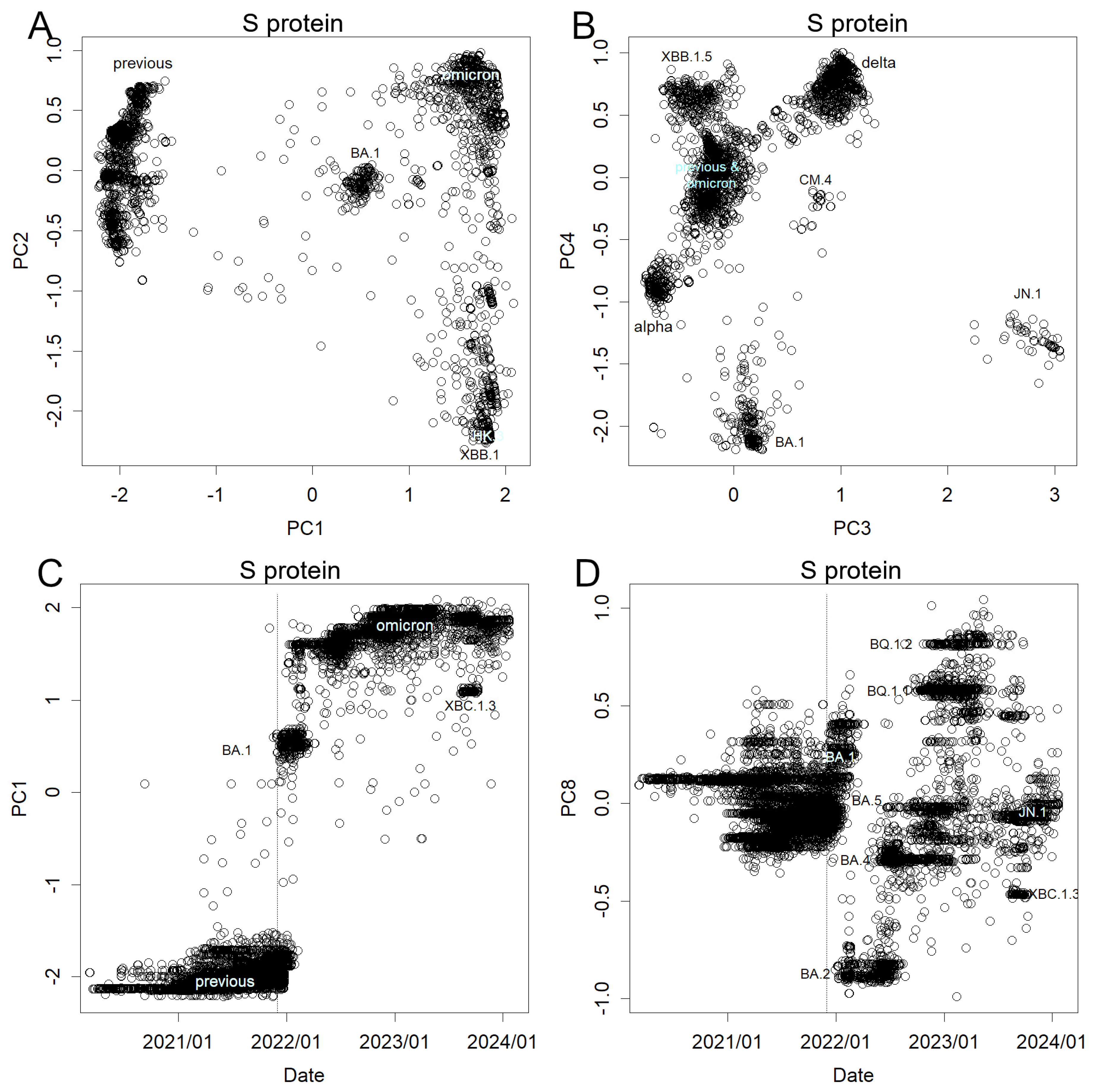
3.3. Mutations Observed in Spike Protein

Alterations of the spike proteins are shown in Figure 3 and Figure S4. As the variability in the mutations diminished by excluding silent mutations, the contribution became more focused on PC1 (Figure S2). Notably, BA.1 resembled the previous variants more closely than in the result of the nucleotide sequence. Presumably, this difference was due to when the axes were set; axes used for the nucleotide sequence were less sensitive to new Omicron variants. Similar to nucleotides, protein mutations manifest abruptly, resulting in discrete clusters, as exemplified by the XBC.1.3 (Figure 3C). Remarkably, instances of stacking of mutations were infrequent; however, an exception was evident in PC8 (stacking from BA.2 to BQ.1.2, depicted in Figure 3D), indicating that BA.1 did not overlay these alterations. Here mutations can be seen stacking up, just like the haemagglutinin mutations in influenza (Figure S1B). However, this is rather an exception (Figures S3 and S4). Previous variants also exhibited analogous shifts along this axis; however, mutations in subsequent variants diverged from this pattern. It is worth mentioning that JN.1 occupies a unique position in PCs 3 and 4 because the mutation responsible for its emergence is fundamentally distinct from preceding mutations (Figure 3B). This became visible because of the new axes, but it is noteworthy that the changes have been large enough to occupy such a high level of PCs and some lower PCs (Figure S4).

It is important to note that the range width of PCs is almost the same for influenza (Figure S1) and SARS-CoV-2, although influenza has a higher concentration of contribution to higher PCs. Hemagglutinin is shorter than the S protein by about half the length, so the proportion altered is higher in the former. However, a similar number of amino acid variations were observed. Influenza has accumulated for 35 years, while SARS-CoV-2 is only one-tenth. This indicated that the latter mutated rapidly.

3.4. Mutated Sites in Spike Proteins in the 3D Structure

The positions that have changed in the 3D structure are shown (Figure 4 and Figure S5). In SARS-CoV-2, most mutations are on the outer side of the spike, but some are on the inner side. In particular, as can be seen in 3D, some residues remain unchanged on the outside, although this may be due to the conservative nature of binding to ACE2 (see Figure S5, which can be rotated in and out). In contrast, in hemagglutinin, the inner residues that are thought to be important for subunit binding are not mutated. Many of the outer residues were altered before being replaced by the Pdm09 strain.

4. Discussion

The Omicron variant exhibited significant mutations at sites not previously mutated in earlier strains (Figure 1), resulting in a different direction of change. This is likely to have facilitated the infection of previously inaccessible people, leading to a surge in patients. Similarly, JN.1 emerged with substantial changes at previously unmutated sites (Figure 3), with many of the mutations inherited from BA.1 lost, indicating a new direction of mutation.

COVID-19 and influenza were quite different in their epidemics. Influenza saw a continuous evolution of a single variant from 1975 to 2009, with mutations accumulating over time. If mutations accumulate in this manner (similar to a random walk), each PC appears as a sin wave, PC1 as a half-wavelength, PC2 as a cycle, PC3 as 1.5 cycles, and so on; lower levels of PCs cover recurrent mutations and frequently replaced mutations. This scenario was observed in influenza (Figure S1) [16]. PC1 monotonically increased (Figure S1A), and PC2 demonstrated mutations and reversions, resulting in a clockwise rotation of PC1 and PC2 when compared annually (Figure S1B). Perhaps influenza infects nearly everyone (though only a small portion become symptomatic) due to its ability to bind to common sialic acid receptors in humans [16]. Therefore, there is basically only one variant of influenza that is prevalent each year. Many people will be immune, so the variant cannot spread again the following year. The following year it will be prevalent elsewhere and mutate a little. After a few years, when enough mutations have accumulated, it returns and causes an epidemic again. Figure 4B and Figure S1 show the result of this accumulation after about 35 years.

In contrast, a certain variant of SARS-CoV-2 infects far fewer individuals [25,26]. For instance, the XBC.1.3 strain had a short-lived prevalence with a limited number of cases (Figure 1B). Consequently, infection rates fluctuate, and the number of cases per wave remains substantially smaller relative to the total population. These minor outbreaks characterize individual variants, leading PCA to detect them along one of its axes. Consequently, the contribution of each axis is markedly small (Figure S2). This is likely due to the spike protein of SARS-CoV-2 binding to ACE2 [4], a protein presented by human cells; naturally, ACE2 exhibits polymorphism, affecting the efficiency of viral binding and resulting in multiple strains circulating simultaneously [27,28]. As each variant undergoes mutations independently, these mutations do not necessarily accumulate. New variants appear suddenly, irrespective of previous variants (Figure 1, Figure 2 and Figure 3, Figures S3 and S4). Consequently, many individuals may lack immunity to a particular mutation, increasing the likelihood of recurrent appearances of the mutation. Moreover, ample room for further mutations remains evident (Figure 4 and Figure S5), suggesting a continued potential for this protein to evade immunity.

SARS-CoV-2 mutates so quickly that primers for PCR to detect it are sometimes disabled [22]. Additionally, mRNA vaccines, which were initially effective, quickly lost their efficacy [25,29,30,31]. The rapid and continuous mutations observed especially in the S protein (Figure 2A) show that it is impractical to target the protein that mutates at such a fast pace for detection or immune response purposes. There are health concerns associated with repeated vaccinations [32,33,34], and this has been confirmed by an increase in IgG4 [35,36,37]. Alternatively, although the effectiveness of suppressing infection may be lower, a vaccine targeting ORF3a, E, and certain regions of N may prevent severe illness, with longer-lasting efficacy. All ORFs of influenza mutate at the same rate [16], so every viral component could be a target for immunity. Of course, similar effects could be achieved using attenuated viruses derived from animal variants, which could be produced without sophisticated technology [38].

The differences in mutations between influenza and SARS-CoV-2, such as the presence of conserved ORFs and the lack of mutation accumulation, suggest distinct selective pressures governing their evolution. Influenza faces selection pressure aimed at evading acquired immunity, allowing only sufficiently mutated variants to drive subsequent outbreaks. Consequently, mutations accumulate. In contrast, humans had no immunity against SARS-CoV-2; only those who had received the mRNA vaccine were immune to the S protein. Thus, the S protein underwent concentrated mutations (Figure 2A). In immunology studies, it is disclosed that this makes the previously acquired immunity less effective [4,5,6,7,8,9]. Reduced serum neutralization was easier to observe, probably due to the limited number of sera that had to be contrasted before and after vaccinations. In comparison, if the same thing were to be done with influenza, for example, one would have to examine sera that change from year to year. Above all, the change in this protein allowed people with a different ACE2 to be infected, which would have created a selection pressure [4,9,27,28]. Hence, several variants were prevalent at the same time, and new mutations occurred independently of each other. This is probably why the mutations have not accumulated (Figure 2). The protein still has a lot of room for mutation (Figure 4 and Figure S5). Furthermore, it is likely that epidemics will continue, mainly among people who have not been previously infected. Moreover, until a convergence of the epidemic is confirmed, public health measures should not be abandoned.

The JN.1 variant, which emerged relatively recently, demonstrates distinct characteristics compared to earlier iterations of Omicron. Notably, it harbors a mutation not found in either the historical record of Omicron or its precursor variants (Figure 3B). Moreover, JN.1 abolishes many mutations typical of BA.1 and other Omicron variants, showing greater similarity to earlier variants (see Figure 1A). Previous observations have indicated low virulence in early Omicron variants [25], likely due to these mutations. Indeed, an increase in hospitalizations has been observed since the emergence of JN.1 [39], possibly linked to the abolition of these mutations. Some report no significant difference in symptoms [40], while others report significantly higher infectivity [41]. This variant appears to have surpassed previous Omicron outbreaks, following a trajectory similar to that of BA.1 (see Figure 1B). If derivatives of this variant continue to replace Omicron and trigger outbreaks, it may be prudent to designate it as Pi for precautionary purposes. Perhaps omicrons are a variant that evolved to evade acquired immunity from early mRNA vaccines [4,5,6,7,8,9]. JN.1. may have corresponded to a vaccine that immunizes omicrons; in any case, this could furthermore be transmitted through different variants of ACE2 [8,41,42].

When looking at PC_items, it is possible to see which nucleotide or amino acid is involved in which mutation, but we did not touch upon this topic here. This is because it does not deal with biochemical data, and therefore cannot provide support for its content; for example, which bases were involved in what properties of the virus. All we have shown here are the facts of how the bases have changed.

References

- WHO. Coronavirus Disease (COVID-19) Pandemic. Available online: https://www.who.int/emergencies/diseases/novel-coronavirus-2019 (accessed on 23 May 2023).
- Konishi, T. Mutations in SARS-CoV-2 are on the increase against the acquired immunity. PLoS ONE 2022, 17, e0271305. [Google Scholar] [CrossRef] [PubMed]
- Wolf, J.M.; Wolf, L.M.; Bello, G.L.; Maccari, J.G.; Nasi, L.A. Molecular evolution of SARS-CoV-2 from December 2019 to August 2022. J. Med. Virol. 2023, 95, e28366. [Google Scholar] [CrossRef]
- Zhang, H.; Lv, P.; Jiang, J.; Liu, Y.; Yan, R.; Shu, S.; Hu, B.; Xiao, H.; Cai, K.; Yuan, S.; et al. Advances in developing ACE2 derivatives against SARS-CoV-2. Lancet Microbe. 2023, 4, e369–e378. [Google Scholar] [CrossRef] [PubMed]
- Cao, Y.; Jian, F.; Wang, J.; Yu, Y.; Song, W.; Yisimayi, A.; Wang, J.; An, R.; Chen, X.; Zhang, N.; et al. Imprinted SARS-CoV-2 humoral immunity induces convergent Omicron RBD evolution. Nature 2023, 614, 521–529. [Google Scholar] [CrossRef] [PubMed]
- Ito, J.; Suzuki, R.; Uriu, K.; Itakura, Y.; Zahradnik, J.; Kimura, K.T.; Deguchi, S.; Wang, L.; Lytras, S.; Tamura, T.; et al. Convergent evolution of SARS-CoV-2 Omicron subvariants leading to the emergence of BQ.1.1 variant. Nat. Commun. 2023, 14, 2671. [Google Scholar] [CrossRef]
- Wang, Q.; Iketani, S.; Li, Z.; Liu, L.; Guo, Y.; Huang, Y.; Bowen, A.D.; Liu, M.; Wang, M.; Yu, J.; et al. Alarming antibody evasion properties of rising SARS-CoV-2 BQ and XBB subvariants. Cell 2023, 186, 279–286.e8. [Google Scholar] [CrossRef] [PubMed]
- Yang, S.; Yu, Y.; Xu, Y.; Jian, F.; Song, W.; Yisimayi, A.; Wang, P.; Wang, J.; Liu, J.; Yu, L.; et al. Fast evolution of SARS-CoV-2 BA.2.86 to JN.1 under heavy immune pressure. Lancet Infect. Dis. 2024, 24, e70–e72. [Google Scholar] [CrossRef]
- Jian, F.; Feng, L.; Yang, S.; Yu, Y.; Wang, L.; Song, W.; Yisimayi, A.; Chen, X.; Xu, Y.; Wang, P.; et al. Convergent evolution of SARS-CoV-2 XBB lineages on receptor-binding domain 455–456 synergistically enhances antibody evasion and ACE2 binding. PLoS Pathog. 2023, 19, e1011868. [Google Scholar] [CrossRef] [PubMed]
- Yao, Z.; Zhang, L.; Duan, Y.; Tang, X.; Lu, J. Molecular insights into the adaptive evolution of SARS-CoV-2 spike protein. J. Infect. 2024, 88, 106121. [Google Scholar] [CrossRef]
- Magazine, N.; Zhang, T.; Wu, Y.; McGee, M.C.; Veggiani, G.; Huang, W. Mutations and Evolution of the SARS-CoV-2 Spike Protein. Viruses 2022, 14, 640. [Google Scholar] [CrossRef]
- Focosi, D.; Quiroga, R.; McConnell, S.; Johnson, M.C.; Casadevall, A. Convergent Evolution in SARS-CoV-2 Spike Creates a Variant Soup from Which New COVID-19 Waves Emerge. Int. J. Mol. Sci. 2023, 24, 2264. [Google Scholar] [CrossRef]
- Zabidi, N.Z.; Liew, H.L.; Farouk, I.A.; Puniyamurti, A.; Yip, A.J.W.; Wijesinghe, V.N.; Low, Z.Y.; Tang, J.W.; Chow, V.T.K.; Lal, S.K. Evolution of SARS-CoV-2 Variants: Implications on Immune Escape, Vaccination, Therapeutic and Diagnostic Strategies. Viruses 2023, 15, 944. [Google Scholar] [CrossRef] [PubMed]
- Zahradník, J.; Nunvar, J.; Schreiber, G. Perspectives: SARS-CoV-2 Spike Convergent Evolution as a Guide to Explore Adaptive Advantage. Front. Cell. Infect. Microbiol. 2022, 12, 748948. [Google Scholar] [CrossRef]
- WHO. Tracking SARS-CoV-2 Variants. Available online: https://www.who.int/en/activities/tracking-SARS-CoV-2-variants/ (accessed on 7 April 2024).
- Konishi, T. Re-evaluation of the evolution of influenza H1 viruses using direct PCA. Sci. Rep. 2019, 9, 19287. [Google Scholar] [CrossRef]
- R Core Team. R: A Language and Environment for Statistical Computing; R Foundation for Statistical Computing: Vienna, Austria, 2020; Available online: https://cran.r-project.org/ (accessed on 7 April 2024).
- Elbe, S.; Buckland-Merrett, G. Data, disease and diplomacy: GISAID’s innovative contribution to global health. Glob. Chall. 2017, 1, 33–46. [Google Scholar] [CrossRef]
- Wright, E.S. DECIPHER: Harnessing local sequence context to improve protein multiple sequence alignment. BMC Bioinform. 2015, 16, 322. [Google Scholar] [CrossRef]
- Yan, R.H.; Zhang, Y.Y.; Li, Y.N.; Ye, F.F.; Guo, Y.Y.; Xia, L.; Zhong, X.Y.; Chi, X.M.; Zhou, Q. S Protein of SARS-CoV-2 in the Active Conformation. Available online: https://www.wwpdb.org/pdb?id=pdb_00007dwz (accessed on 7 April 2024).
- Berman, H.M.; Westbrook, J.; Feng, Z.; Gilliland, G.; Bhat, T.N.; Weissig, H.; Shindyalov, I.N.; Bourne, P.E. The Protein Data Bank. Nucleic Acids Res. 2000, 28, 235–242. [Google Scholar] [CrossRef]
- Heo, C.-K.; Lim, W.-H.; Yang, J.; Son, S.; Kim, S.J.; Kim, D.-J.; Poo, H.; Cho, E.-W. Novel S2 subunit-specific antibody with broad neutralizing activity against SARS-CoV-2 variants of concern. Front. Immunol. 2023, 14, 1307693. [Google Scholar] [CrossRef] [PubMed]
- Murdoch, D.; Adler, D.; Nenadic, O.; Urbanek, S.; Chen, M.; Gebhardt, A.; Bolker, B.; Csardi, G.; Strzelecki, A.; Senger, A.; et al. rgl: 3D Visualization Using OpenGL. Available online: https://cran.r-project.org/web/packages/rgl/index.html (accessed on 7 April 2024).
- Konishi, T. Continuous mutation of SARS-CoV-2 during migration via three routes. PeerJ 2022, 10, e12681. [Google Scholar] [CrossRef] [PubMed]
- Konishi, T. A Comparative Analysis of COVID-19 Response Measures and Their Impact on Mortality Rate. COVID 2024, 4, 130–150. [Google Scholar] [CrossRef]
- Konishi, T. COVID-19 Epidemics Monitored Through the Logarithmic Growth Rate and SIR Model. J. Clin. Immunol. Microbiol. 2022, 3, 1–45. [Google Scholar] [CrossRef]
- Suryamohan, K.; Diwanji, D.; Stawiski, E.W.; Gupta, R.; Miersch, S.; Liu, J.; Chen, C.; Jiang, Y.-P.; Fellouse, F.A.; Sathirapongsasuti, J.F.; et al. Human ACE2 receptor polymorphisms and altered susceptibility to SARS-CoV-2. Commun. Biol. 2021, 4, 475. [Google Scholar] [CrossRef] [PubMed]
- Sano, E.; Deguchi, S.; Sakamoto, A.; Mimura, N.; Hirabayashi, A.; Muramoto, Y.; Noda, T.; Yamamoto, T.; Takayama, K. Modeling SARS-CoV-2 infection and its individual differences with ACE2-expressing human iPS cells. iScience 2021, 24, 102428. [Google Scholar] [CrossRef] [PubMed]
- Buchan, S.A.; Chung, H.; Brown, K.A.; Austin, P.C.; Fell, D.B.; Gubbay, J.B.; Nasreen, S.; Schwartz, K.L.; Sundaram, M.E.; Tadrous, M.; et al. Estimated Effectiveness of COVID-19 Vaccines Against Omicron or Delta Symptomatic Infection and Severe Outcomes. JAMA Netw. Open 2022, 5, e2232760. [Google Scholar] [CrossRef] [PubMed]
- Hansen, C.H.; Schelde, A.B.; Moustsen-Helm, I.R.; Emborg, H.-D.; Krause, T.G.; Mølbak, K.; Valentiner-Branth, P.; on behalf of the Infectious Disease Preparedness Group at Statens Serum Institut. Vaccine effectiveness against SARS-CoV-2 infection with the Omicron or Delta variants following a two-dose or booster BNT162b2 or mRNA-1273 vaccination series: A Danish cohort study. medRxiv 2021. [Google Scholar] [CrossRef]
- Pérez-Then, E.; Lucas, C.; Monteiro, V.S.; Miric, M.; Brache, V.; Cochon, L.; Vogels, C.B.F.; Malik, A.A.; De la Cruz, E.; Jorge, A.; et al. Neutralizing antibodies against the SARS-CoV-2 Delta and Omicron variants following heterologous CoronaVac plus BNT162b2 booster vaccination. Nat. Med. 2022, 28, 481–485. [Google Scholar] [CrossRef] [PubMed]
- Gao, F.X.; Wu, R.X.; Shen, M.Y.; Huang, J.J.; Li, T.T.; Hu, C.; Luo, F.Y.; Song, S.Y.; Mu, S.; Hao, Y.N.; et al. Extended SARS-CoV-2 RBD booster vaccination induces humoral and cellular immune tolerance in mice. iScience 2022, 25, 105479. [Google Scholar] [CrossRef] [PubMed]
- Gruell, H.; Vanshylla, K.; Tober-Lau, P.; Hillus, D.; Schommers, P.; Lehmann, C.; Kurth, F.; Sander, L.E.; Klein, F. mRNA booster immunization elicits potent neutralizing serum activity against the SARS-CoV-2 Omicron variant. Nat. Med. 2022, 28, 477–480. [Google Scholar] [CrossRef] [PubMed]
- Harvey, W.T.; Carabelli, A.M.; Jackson, B.; Gupta, R.K.; Thomson, E.C.; Harrison, E.M.; Ludden, C.; Reeve, R.; Rambaut, A.; Peacock, S.J.; et al. SARS-CoV-2 variants, spike mutations and immune escape. Nat. Rev. Microbiol. 2021, 19, 409–424. [Google Scholar] [CrossRef] [PubMed]
- Irrgang, P.; Gerling, J.; Kocher, K.; Lapuente, D.; Steininger, P.; Habenicht, K.; Wytopil, M.; Beileke, S.; Schäfer, S.; Zhong, J.; et al. Class switch toward noninflammatory, spike-specific IgG4 antibodies after repeated SARS-CoV-2 mRNA vaccination. Sci. Immunol. 2023, 8, eade2798. [Google Scholar] [CrossRef]
- Kiszel, P.; Sík, P.; Miklós, J.; Kajdácsi, E.; Sinkovits, G.; Cervenak, L.; Prohászka, Z. Class switch towards spike protein-specific IgG4 antibodies after SARS-CoV-2 mRNA vaccination depends on prior infection history. Sci. Rep. 2023, 13, 13166. [Google Scholar] [CrossRef]
- Uversky, V.N.; Redwan, E.M.; Makis, W.; Rubio-Casillas, A. IgG4 Antibodies Induced by Repeated Vaccination May Generate Immune Tolerance to the SARS-CoV-2 Spike Protein. Vaccines 2023, 11, 991. [Google Scholar] [CrossRef] [PubMed]
- Konishi, T. SARS-CoV-2 mutations among minks show reduced lethality and infectivity to humans. PLoS ONE 2021, 16, e0247626. [Google Scholar] [CrossRef] [PubMed]
- National Institute of Infectious Diseases, Japan. New Coronavirus Infectious Disease Surveillance News/Weekly Report: Understand the Status of Outbreak Trends. Available online: https://www.niid.go.jp/niid/ja/2019-ncov/2484-idsc/12015-covid19-surveillance-report.html (accessed on 7 April 2024).
- Katella, K. 3 Things to Know About JN.1, the New Coronavirus Strain. Available online: https://www.yalemedicine.org/news/jn1-coronavirus-variant-covid (accessed on 7 April 2024).
- Kaku, Y.; Okumura, K.; Padilla-Blanco, M.; Kosugi, Y.; Uriu, K.; Hinay, A.A., Jr.; Chen, L.; Plianchaisuk, A.; Kobiyama, K.; Ishii, K.J.; et al. Virological characteristics of the SARS-CoV-2 JN.1 variant. Lancet Infect. Dis. 2024, 24, e82. [Google Scholar] [CrossRef] [PubMed]
- Sohail, M.S.; Ahmed, S.F.; Quadeer, A.A.; McKay, M.R. Cross-Reactivity Assessment of Vaccine-Derived SARS-CoV-2 T Cell Responses against BA.2.86 and JN.1. Viruses 2024, 16, 473. [Google Scholar] [CrossRef] [PubMed]
Figure 1.
Mutations observed from nucleotide sequence. The axes were found at the end of 2021 when BA.1 emerged. Note the Pango Lineage of the groups that stood out, which was provided by GISAID. (A) PC1 and PC2. BA.1 and Omicron were largely separated by mutations not seen in the previous variants, forming PC1. Some features of BA.1 were inherited by subsequent Omicron variants. However, XBC1.3 and JN.1 have reverted from the shared mutations and are closer to the former variants. (B) Time course of PC1. BA.1 appeared after 1 December 2021, indicated by the dotted line, and the former variants were almost absent. This was then replaced by a population of Omicron variants, which eventually moved to JN.1.
Figure 2.
The standard deviation of how much each base has mutated since the beginning of the epidemic: (A) Large ORFs. (B) Small ORFs. In the spike protein, most bases are mutated, especially at the N-terminus. Some smaller ORFs are also highly altered. However, 3a and E were conservative.
Figure 3.
Mutations were observed in the amino acid sequence of the S protein. (A) PC1 and 2, note the position of BA.1 (B) PC3 and 4, see that JN.1 differs from others in the directions presented here. (C) Time course of PC1. Time course of (D) PC8, a rare case that shows stacking of mutations.
Figure 4.
The site of mutation is represented on the 3D model of the protein: (A) S protein of SARS-CoV-2, (B) haemagglutinin of influenza H1N1. Each protein is made up of the association of three identical subunits, shown in different colors; mutations are shown in blue on one subunit. For more details, see Figure S5, which can be moved.
Disclaimer/Publisher’s Note: The statements, opinions and data contained in all publications are solely those of the individual author(s) and contributor(s) and not of MDPI and/or the editor(s). MDPI and/or the editor(s) disclaim responsibility for any injury to people or property resulting from any ideas, methods, instructions or products referred to in the content. |
© 2024 by the authors. Licensee MDPI, Basel, Switzerland. This article is an open access article distributed under the terms and conditions of the Creative Commons Attribution (CC BY) license (https://creativecommons.org/licenses/by/4.0/).
Share and Cite
MDPI and ACS Style
Konishi, T.; Takahashi, T. Mutation Trajectory of Omicron SARS-CoV-2 Virus, Measured by Principal Component Analysis. COVID 2024, 4, 571-581. https://doi.org/10.3390/covid4040038
AMA Style
Konishi T, Takahashi T. Mutation Trajectory of Omicron SARS-CoV-2 Virus, Measured by Principal Component Analysis. COVID. 2024; 4(4):571-581. https://doi.org/10.3390/covid4040038
Chicago/Turabian StyleKonishi, Tomokazu, and Toa Takahashi. 2024. "Mutation Trajectory of Omicron SARS-CoV-2 Virus, Measured by Principal Component Analysis" COVID 4, no. 4: 571-581. https://doi.org/10.3390/covid4040038