
Approach to Equilibrium of Statistical Systems: Classical Particles and Quantum Fields Off-Equilibrium


Departamento de Física Teórica, Universidad Complutense de Madrid, 28040 Madrid, Spain
Dynamics 2023, 3(2), 345-378; https://doi.org/10.3390/dynamics3020020
Submission received: 3 April 2023
/
Revised: 5 June 2023
/
Accepted: 7 June 2023
/
Published: 13 June 2023
Abstract
:Non-equilibrium evolution at absolute temperature T and approach to equilibrium of statistical systems in long-time (t) approximations, using both hierarchies and functional integrals, are reviewed. A classical non-relativistic particle in one spatial dimension, subject to a potential and a heat bath (), is described by the non-equilibrium reversible Liouville distribution (W) and equation, with a suitable initial condition. The Boltzmann equilibrium distribution generates orthogonal (Hermite) polynomials in momenta. Suitable moments of W (using the ’s) yield a non-equilibrium three-term hierarchy (different from the standard Bogoliubov–Born–Green–Kirkwood–Yvon one), solved through operator continued fractions. After a long-t approximation, the ’s yield irreversibly approach to equilibrium. The approach is extended (without ) to: (i) a non-equilibrium system of N classical non-relativistic particles interacting through repulsive short range potentials and (ii) a classical field theory (without ). The extension to one non-relativistic quantum particle (with ) employs the non-equilibrium Wigner function (): difficulties related to non-positivity of are bypassed so as to formulate approximately approach to equilibrium. A non-equilibrium quantum anharmonic oscillator is analyzed differently, through functional integral methods. The latter allows an extension to relativistic quantum field theory (a meson gas off-equilibrium, without ), facing ultraviolet divergences and renormalization. Genuine simplifications of quantum theory at high T and large distances and long t occur; then, through a new argument for the field-theoretic case, the theory can be approximated by a classical one, yielding an approach to equilibrium.
1. Introduction
Many fundamental issues continue to be open in the extensive avenues leading from equilibrium statistical mechanics [1,2,3,4,5,6,7,8] to non-equilibrium statistical mechanics [8,9,10,11,12,13,14,15,16] in both classical and quantum regimes.
Off-equilibrium evolution of statistical systems displays stochasticity: see [17,18,19] in the classical domain and [20,21,22,23,24,25,26] in the quantum one, specifically in the theory of open quantum systems. For further background in classical (thermodynamical) frameworks, see [27,28,29,30].
Our leading motivation has been to study the possible approach to equilibrium of various statistical system, under suitable approximations, for very long time t.
Previous authors have employed infinite hierarchies in the analysis of several stochastic equations [31,32].
The present author has analyzed the classical Liouville and quantum Wigner equations, by using infinite hierarchies in order to implement approaches to equilibrium [33,34,35,36,37,38,39,40,41]. The analysis has been extended, using different techniques (generating functionals), to off-equilibrium evolution in the relativistic quantum field theory [42,43]. The above approaches face various complications, which have been treated succesively.
Based upon those works, the present work will review, from a first principles standpoint, the evolution of certain statistical classical and quantum systems in some non-equilibrium states at the initial time and their approximate off-equilibrium development for long time . The evolution will be supposed to proceed at given absolute temperature T, in the following sense: (i) either the system is small and evolves subject to an external heat bath () or (ii) it has a very large (or infinite) number of degrees of freedom, a large part of them being at equilibrium at T, while the remaining ones are not and so are responsible for the off-equilibrium evolution. In case (i), we omit any analysis of the states of the , and we focus exclusively on the states of the system considered. Ab initio dissipation is excluded, by assumption, in all cases (vanishing friction due to any other system).
Section 2 begins with a one-dimensional statistical system, namely, one classical non-relativistic particle subject to an external potential and to a at thermal equilibrium. Section 2 also deals with a closed classical non-relativistic many-particle system, in three spatial dimensions: the particles interact among themselves without any external , with initial states describing thermal equilibrium at large distances but non-equilibrium at finite ones.
In order to illustrate some difficulties of the approach in Section 2 and Section 3 in the quantum case and how they could be bypassed under certain approximations, Section 4 studies, with less detail, a one-dimensional statistical system, namely, the quantum version of the one in Section 2. Rather wide references provide developments omitted here.
By avoiding the strategy in Section 2, Section 3 and Section 4, and as an introduction to the power of the functional methods to be employed profusely in Section 6, Section 5 treats a quantum anharmonic oscillator in which no ultraviolet divergences are present.
Section 6 is devoted to relativistic quantum field theory. Various approaches to the non-equilibrium quantum meson gas are summarized. General problems with initial non-equilibrium states at finite time are described in outline. The overview to be presented will enable the discussion of the quantum-field-theoretic framework at certain stages and under certain conditions, and the approximate approach to equilibrium, through a new argument, so as to connect with Section 3. Suitable references give derivations omitted here.
The contents of the successive sections have been described above in a somewhat sketchy way so as not to burden this introduction. The reader could proceed directly to Section 7, which offers a less sketchy account of Section 2, Section 3, Section 4, Section 5 and Section 6, summarizes the work, and presents the conclusions. Some open problems are highlighted in Section 7.
This feature article presents globally consistent consequences for the systems considered in it. Computations and derivations will be omitted by referring to suitable references.
2. Classical Particle Systems
2.1. Open Classical One Particle Systems
Methods in the hierarchy approach, to be also used in Section 3 and Section 4, will be introduced in this section.
2.1.1. One-Dimensional Case: Some General Aspects
Let a classical particle, with mass m, position x and momentum q, be subject to a real potential , in the presence of a heat bath () at thermal equilibrium at absolute temperature T. We shall employ the standard variable ( being Boltzmann’s constant).
By assumption, the potential is repulsive: : either as or . The Hamiltonian of the particle is: . Let the classical particle be, at the initial time , out of thermal equilibrium with the , and have a Liouville probability distribution function (≥0) to be at x with momentum q. Then, the non-equilibrium particle could be, at time t(>0), at x with momentum q, with probability distribution (≥0).
As an example, the classical particle could be a virus or a grain of pollen, performing Brownian motion in air (at rest and at thermal equilibrium, at K) in a room. Air would be the .
The (time-reversible or, simply, reversible) Liouville equation accounts for the time evolution of W:
with the initial condition . The equilibrium (Boltzmann’s) distribution, the t-independent solution of Equation (1) describing thermal equilibrium of the particle with the , is
which is Gaussian in q.
Let be the momentum scale determined by T. With , let us introduce the denumerably infinite family of all (unnormalized) polynomials in y: (), the standard n-th Hermite polynomial [44]. They are orthogonalized in y (for fixed x) by using as (Gaussian) weight function. With , one has, for and any x (left unintegrated):
The orthonormalized polynomials are
is the marginal probability distribution for x. If , then and , Equation (3) can also be applied to the initial off-equilibrium distribution and gives the initial moments, . One has the following (formal) expansion for W:
2.1.2. Three-Term Hierarchy and Operator-Continued Fractions
Equations (1)–(3) give rise to an exact three-term non-equilibrium hierarchy for all ’s. It is more convenient to replace the latter by the symmetrized moments
Then, the hierarchy for the ’s becomes directly the following exact three-term (reversible) hierarchy for the ’s, for any n:
with initial condition . One crucial property is that the operators and are the adjoint of each other.
Let the Laplace transform
be performed. Its inverse is
(c being real and being analytic in the half-plane of the complex s-plane). This definition and Equation (5) gives rise to the three-term hierarchy for :
The hierarchy in Equation (7) can be solved through a formally direct extension of standard methods for dealing with numerical three-term linear recurrence relations in terms of continued fractions (see, for instance, [17]). Such a formal procedure yields all , for any , in terms of sums of products of certain s-dependent linear (integral) operators , , which act upon and upon all ’s, with . The linear operators ’s are defined in a recurrent way through:
I is the unit operator. By iteration of Equation (8), becomes a formal infinite continued fraction of products of the linear operators and (which in general do not commute with each other). The formal infinite continued fraction of operators reads:
A simpler hierarchy, without an essential loss of generality, follows by assuming, except otherwise stated, that for , with .
2.1.3. Properties of
Let us choose n(≥1) and fix (real and suitably small) in any . Then, the following crucial properties appear to hold (in general, for either or ) [33,34]: if were Hermitian, and if all its eigenvalues (which would be real) were non-negative, then the same would hold true for . As an example, it is easy to confirm the validity of that property if and are chosen as matrices, such that be the adjoint of . Then, through iterative arguments, ’s, , turn out to be Hermitian matrices, and all their eigenvalues are non-negative. See [34].
For a better understanding of the operator-continued fractions , we shall take and let (allowing for if desired, later [33]).
Let us perform a spatial Fourier transformation from configuration space (x) to wavevector space (k), by applying . Let . Then, the Fourier transform of the operator-continued fraction in Equation (8), for Re and yields:
By iteration, becomes the following ordinary continued fraction for (involving no non-commuting operators):
to be compared to Equation (9) for (involving non-commuting operators).
For relationships of to the n-th repeated integral of the complementary error function () and the standard Gamma function , see [45].
The various operator-continued fractions behave, on average, as for large n: we shall omit details [33]. For , diverges as (due to ). Then, also diverges near (as the actual system is one-dimensional).
2.1.4. Long-Time (t) Approximation
The long-t approximation for reads in general (that is, without imposing for , with ) as follows. One replaces for any yielding in terms of by : this approximation is not performed for , which will be crucial, and is the better, the larger . We regard for as a fixed (s-independent) operator. For simplicity, let us continue with the simplification: for , with . Moreover, after the above long-t approximation, we shall continue with the same initial condition at : it may well be that this amounts to another kind of approximation.
Then, for small s, we approximate for as: . The resulting hierarchy for ’s (), through the inverse Laplace transform, yields a closed approximate irreversible hierarchy for , . The solutions of the last closed hierarchy for relax irreversibly, for large t and reasonable , towards and , (thermal equilibrium) [33,34]. For long-t, the dominant moment is , while any with being the smaller, the larger n and are (due to the behaviors of and of with n). Similar behaviors hold for and with .
We shall illustrate the above facts by taking, for simplicity, .
Then, Equation (11) for small s and becomes: (to be compared to Equation (11) before the approximation). Then, Equations (10) and (11) yield, by taking inverse Laplace transforms:
One finds directly the irreversible Smoluchowski equation for the moment, as a result:
with initial condition .
The right-hand side of Equation (16) should be interpreted as:
. Let for suitable functions and . Due to the Hermiticity of , is Hermitian (all eigenvalues of being ≥0). Let be an eigenfunction of the integral operator with eigenvalue (≥ 0). Then,
is a short-hand notation denoting integration and summation over the whole spectrum of .
By expanding , with x-independent , the solution of (16), with the above initial condition, is
which relaxes irreversibly as towards , corresponding to . At equilibrium, one has , and , , consistently. Then, Equation (16) is (at least, with ) irreversible: for long t(>0) the dominant moment is , while any with is negligible, being the smaller, the larger n and t(>0), and so on for the ’s.
As an example of the relaxation towards equilibrium, we consider the solution of Equation (16) for (, harmonic oscillator), and initial condition , denoting the Dirac delta function. One obtains (, being regarded as a positive constant):
For ,
, which is proportional to . The t-behavior of G is represented in Figure 1, in order to display the relaxation for .
Irreversible thermalization does not happen in the absence of long-t approximations. Then, the above approximations ( for , but not for ), giving rise to the thermalization with the (as implemented in Equation (16)), is an alternative way of introducing irreversibility out of the reversible Equation (1).
2.2. Closed Classical Many-Particle Systems: Long-Time Approximation and Arrow of Time
2.2.1. Initial State Motivated by Fluid Dynamics, Hierarchy, and Continued Fractions
See [33]. We treat a closed large system of many () classical identical non-relativistic particles with mass m, in three spatial dimensions, with spatial coordinates ,…, () and momenta ,…, (). Let and be the Cartesian components of and , respectively (, ). The non-equilibrium classical probability distribution function is: .
Assumptions—(a) Neither a nor external friction mechanisms nor external forces are assumed. The system contains a very large set () of degrees of freedom at large distances at thermal equilibrium at absolute temperature T with one another: plays the role of an (internal) . The system is in a non-equilibrium state, because it also contains a large set of degrees of freedom (smaller than ) at finite distances, which are off-equilibrium with the set , and among themselves. Then, the known initial non-equilibrium distribution describes thermal equilibrium at absolute temperature T for the set located at large distances but off-equilibrium for the set located at finite distances [33]. The above qualitative idea will become clearer through , discussed below in (c).
(b) The interaction potential among the particles is and we suppose that all are repulsive (≥0) and tend quickly to zero for large . is the classical N-particle Hamiltonian. Then, Boltzmann’s equilibrium (canonical) distribution at temperature T is .
(c) The initial distribution function , at , will be compatible with the limited information available, namely, with standard variables employed in equilibrium statistical mechanics and fluid dynamics [4,8,12,13,14,46]. will depend on a finite number of (actually, ) functions of one single : , , and , (all of them independent of time and on momenta). in terms of and has appeared previously [8,14] (and is related to the Massieu–Planck function [14]). , describing thermal equilibrium with homogeneous temperature T for large distances (large ) but non-equilibrium for intermediate and short distances (with spatial inhomogeneities), reads
denoting the three-dimensional Dirac delta function. The ’s will be uniquely determined in terms of -dependent observables (also independent of time and on momenta) typically employed in Fluid Dynamics, which, by assumption, are known at : mass density, fluid velocity and some suitable energy density [14,33]. We accept that (constant), as along any direction and that the same holds for and for . The constant limiting values describe equilibrium, with , and . At finite , the off-equilibrium , and do depend on . Consistency is achieved (the temperature T being thereby introduced) if, in the thermodynamical limit, tends to
(plus corrections which approach zero in that limit). For a detailed analysis, see [33].
The reversible Liouville equation reads
Let denote a set of non-negative integers and let . Let . We introduce non-equilibrium moments of W (using products of Hermite polynomials):
If , then () is proportional to and , (say, ). Equation (20) can also be applied to and gives the corresponding initial moments, . We shall work with the symmetrized moments
.
One obtains an infinite reversible three-term linear recurrence for ’s, generalizing Equations (5) and (6):
The Laplace transform of the above N-particle hierarchy Equation can be formally solved in terms of linear operators , which generalize the previous . For details, see [33]. All are square matrices, due to the indices and and also integral operators, arising from the linear operators and , as l, and vary. The fulfill the formal hierarchy (which generalizes Equation (8))
The linear operators are rectangular matrices, formed out of operators and . is the adjoint of [33]. By iterating Equation (23) indefinitely, becomes an operator-continued fraction, which depends on all and and generalizes the operator-continued fraction for .
for is a Hermitian operator with non-negative eigenvalues for [33]. No approximation has been performed so far.
Let . Let us Laplace- and Fourier-transform the above N-particle hierarchy to wavevector space (, …, ). Let
Then, the Fourier transform of for Re yields an ordinary continued fraction, given in Equations (12) and (13) with replaced by . Then, with such a replacement, the properties of given in Section 2.1.3 also hold for . Notice that diverges as if . On the other hand, and contrary to what happened for one particle in one spatial dimension (recall the comment in Section 2.1.3), converges near . The approximate ansatz in [40] can be extended readily to .
2.2.2. Long-Time Approximation and Consequences
A simple long-time approximation can be performed in the dynanical equation for , for (and vanishing quickly at large distances) and very large N (eventually, in the thermodynamical limit), which generalizes the one in Section 2.1.4. This approximation consists in fixing ( being small) in the whole hierarchy of operators , for any
which, then, become Hermitian operators with no negative eigenvalues. It is crucial that s-dependences be kept in , for .
The non-vanishing factors and
in
respectively, tend to reduce, as the ’s increase, the importance of ’s with fixed and . This is a genuine feature of the ’s. See [33], where it was shown that by imposing , the long-t approximation is still exactly consistent with all (five) hydrodynamical balance equations. For simplicity, we discard all the initial moments for .
We regard as a fixed (s-independent) operator, yielding all in terms of all . Moreover, after the above long-t approximation, we shall continue with the same initial condition at : it may amount to another kind of approximation.
All that leads to a closed approximate hierarchy for ’s, which appears to yield an approximate irreversible evolution towards thermal equilibrium at T. ’s and, then, relax the quicker the larger n. would dominate the approach towards equilibrium for . See [33]. All that appears to work for fixed .
Let : see [33] for . One finds the irreversible Smoluchowski-like equation for the moment, which generalizes (16) ( meaning
The operator (Hermitian, with non-negative eigenvalues) has, as a square matrix, the matrix elements . The initial condition is .
Discussion and consequences—(a) the exact hierarchy for the ’s and the closed approximate one for them after the long-t approximation are genuinely different from the non-equilibrium classical Bogoliubov–Born–Green–Kirkwood–Yvon (BBGKY) hierarchy [12,13]. (b) The structure of (24), with replaced by a constant, is similar to that of the linear Smoluchowski equation in the standard Rouse model for polymer dynamics [47]. (c) The following t-dependent function, for generic :
(the integration over any being performed in ) fulfills
which could characterize an arrow of time. L is a Liapunov function. See [41].
3. Classical Scalar Massive Field
3.1. Hamiltonian and Liouville Equation
In dimensions (t, real time and , three-dimensional spatial coordinates), let a large statistical system, with dynamics described by a real relativistic scalar classical field , with mass parameter m; and coupling constant g. See [35].
The classical Hamiltonian is supposed to be: . is the field momentum and . We shall include an upper limit or ultraviolet cut-off () on the magnitude of any contributing wavevector in an eventual Fourier transform of . Unless otherwise stated, . No external heat bath will be assumed: like in Section 2.2, the infinite number of degrees of freedom of this classical field system gives rise to statistical effects. Let be the classical probability distribution function for the system at time t to be described by the field configuration with momentum . W fulfills the classical reversible Liouville equation, which reads
where denotes functional derivative. Let: be an initial non-equilibrium distribution at time , containing a spatial inhomogeneity characterized by a function : could be interpreted, at least qualitatively, as proportional to the absolute temperature of a small volume (at the macroscopic scale) at . It is supposed that for large , the field degrees of freedom are at thermal equilibrium at absolute temperature T: compare with Section 2.2. Accordingly, for large , with .
3.2. Non-Equilibrium Moments and Approximate Irreversible Evolution
Let and . Functional Hermite polynomials are introduced through the Rodrigues-like formula:
Moments of W are introduced through the functional integral:
The developments in Section 2 can be extended to generate a three-term hierarchy for (symmetrized moments determined by) the moments , operator continued fractions and so on. Through long-t approximations, the following irreversible functional Fokker–Planck equation for the lowest moment holds:
with constant D and . As , Equation (31) yields the equilibrium solution . Up to this stage, . and, so, the classical field theory defined by Equation (31) contain ultraviolet divergences as the cut-off . Those divergences can be absorbed and eliminated by the so-called mass renormalization: one sets , where is finite. is introduced so as to absorb the ultraviolet divergences generated and, so, is divergent as . After such an absorption and since neither g nor require renormalization, all correlation functions determined by W are ultraviolet finite. For discussions and details, see [35,36,37] and references therein. The classical theories associated to Equations (27) and (31) could give rise to divergences of a different nature, namely, field energies divergent as . Such divergences, could be compensated, at least partially, by renormalization of the energy.
For a generalization of the developments in Section 2 and in this section to a non-equilibrium classical plasma (namely, non-relativistic charged particles interacting with the classical electromagnetic field) (with a fixed ultraviolet cut-off) and its approach to thermal equilibrium at temperature T, see [34].
4. One Quantum Particle Subject to a Heat Bath: Short Discussion
For general aspects on quantum systems subject to a larger heat bath (), see [8,13,14,20,21,22,24,25,26,48,49,50,51,52,53,54,55] and references therein. We accept that the state of the system, for sufficiently long-t, approaches towards its own canonical density operator at thermal equilibrium with the at absolute temperature T, as studied in [48,49,50,51,52,53,54,55]. We will focus exclusively on the quantum states of the system.
Our study here of the quantum one particle case, aimed at comparing the hierarchy approach with the results in [8,13,14,20,21,22,24,25,26,48,49,50,51,52,53,54,55], will display analogies and genuine differences with respect to the classical case (Section 2.1). For the quantum non-relativistic N particle case, see [41], and for the cases in connection with chemical reactions, in the hierarchy approach, see [40,41].
General Aspects
We shall consider one non-relativistic quantum spinless Brownian particle of mass m (>0) and momentum operator , in one spatial dimension x, with (Hermitian) quantum Hamiltonian (ℏ being Planck’s constant):
Assumptions—The real potential fulfills: quickly, as and all , , are continuous for any x, and allow for and, hence, the possibility of bound states of the particle by the potential V. The particle is also subject to the .
The non-equilibrium statistical evolution for is given by the density operator (a statistical mixture of quantum states), with the given initial condition . for and are Hermitian and positive-definite linear operators acting in the Hilbert space spanned by the set of all eigenfunctions of . Unless otherwise stated, we shall not impose that be normalized. One has ():
We consider the matrix element of in generic eigenstates, , , of the quantum position operator. The quantum Wigner function , determined by , is [56,57,58,59,60]:
The initial non-equilibrium Wigner function at is , given by Equation (34) if . For , the exact reversible quantum master equation for [56,57] reads
As , the above Wigner equation becomes formally, by dropping all ℏ-dependent terms (containing , ), the classical Liouville Equation (1), with [56,57].
The equilibrium Wigner function fulfills
is the Wigner function determined by . The Wigner functions W and can be in certain regions. See: reference [61]. In general, there is no compact formula for .
One can introduce the orthogonal polynomials in momentum (q) generated by . The non-positivity of and is bypassed by invoking a suitable extension of the theory of orthogonal polynomials [62]: one assumes [39,40,41] that yields a family of orthogonal polynomials in momentum, in the framework of [62]. The latter generate non-equilibrium moments , like in the classical case: see [39,40,41].
The above non-equilibrium dynamical Wigner equation gives rise to a hierarchy for the non-equilibrium moments . Here, one meets another genuine quantum difficulty: the hierarchy is not a three-.term one and, hence, more difficult to study. This difficulty is bypassed, at least in principle, by searching for regimes enabling to formulate approximately a Schmolukowski equation for the lowest non-equilibrium moment , yielding approach to equilibrium for long t [39]. Those complexities of the present hierarchy framework amplify as one proceeds far from the classical regime, say, towards lower temperatures. So, upon accepting that the state of a quantum system, for sufficiently long t, tends to its equilibrium canonical density operator (in agreement with [8,13,14,20,21,22,24,25,26,48,49,50,51,52,53,54,55]), to derive such an approach in the present hierarchy framework, even if possible in principle, becomes the more complicated the more one detaches from the classical regime.
Conversely, such difficulties tend to simplify (in particular, the hierarchies becoming approximately three-term ones) in a quantum regime which be not far from the classical regime. Specifically, let us consider that T is neither high (so as not to enter entirely in the classical regime) nor low (so as to avoid the low temperature regime). Therefore, we proceed to the regime of typical chemical reactions: small thermal wavelength (small , ). In it, the general non-equilibrium quantum hierarchy [39,40,41] can be approximated by a three-term hierarchy, generalizing Equation (5).
We shall perform the long-t approximation for t longer than a certain largest effective evolution time. We shall omit details, which extend formally the ones in Section 2.1.4. We shall assume that approximately the initial condition gives rise to moments and for . One gets the following irreversible approximate quantum (Smoluchowski-like) equation for the lowest non-equilibrium moment :
with
and .
D being a suitable approximation for combinations of quantum operator-continued fractions, which constitute extensions of Equations (8) and (23) [39,40]. As a zeroth approximation, D can be supposed to be a constant. See Appendix A in [39]. These procedure and approximations are, in principle, independent of (which contains quantum features, as it follows from ).
The result in Equation (35), implying long-t irreversibility, embodies stochasticity and displays a structure typical of diffusion-convection-reaction equations: it is linear, convection is determined by the V-dependent term and external sources are absent. An extension of Equation (35) was used in [40] to study binary chemical reactions. In turn, reference [40] extended a previous one (based on classical statistical mechanics) of the non-equilibrium dynamics of DNA [63].
5. Functional Methods toward Quantum Field Theory: Quantum Anharmonic Oscillator
5.1. Oscillator at Equilibrium through Functional Integrals
A quantum anharmonic oscillator of mass m in one spatial dimension (coordinate ), momentum and frequency will be treated here, based on [42]. The method in Section 4 could be applied to it, but functional methods will be preferred, as an introduction to those to be applied for the quantum field case in Section 6. with is the Hamiltonian operator. g (g(≥0)) denotes the coupling constant. We shall outline its equilibrium statistical mechanics in the presence of an external at thermal equilibrium at equilibrium temperature is included. The equilibrium statistical mechanics of the quantum oscillator is accounted for through the equilibrium density operator: . An external source is introduced depending on the imaginary time () [64,65,66,67]. The generating functional integral for the quantum oscillator at equilibrium with the reads (): [64,65,66,67]:
which is performed with periodic boundary conditions: and with . yields the thermodynamical partition function: . In the regime of high temperature (that is, small ), one assumes that and become -independent: and . Then, Equation (36) describes a classical anharmonic oscillator at equilibrium [37]:
which is an ordinary integral [37].
5.2. Oscillator Off-Equilibrium: Generating Functionals
Let the oscillator be off-equilibrium at the initial time , with the following specific initial density operator (physically interesting in connection with quantum fields off-equilibrium in Section 6):
does correspond to a nonequilibrium initial state if the constant . Thus, if denotes the standard trace operation, one finds: provided that . In Section 6 (the quantum field case), the structures of the initial nonequilibrium states will generalize Equation (38). Initial nonequilibrium states have been considered, for instance in [14].
The density operator determines the time evolution for , and the superscript denoting the evolution operator and the adjoint, respectively. We shall suppose a suitably large time T (not to be confused here with absolute temperature) much larger than any time t of physical interest: . will denote an arbitrary eigenstate of the coordinate operator . By introducing two complete sets of intermediate eigenstates and of , one obtains: . That enables to represent and by means of real-time functional integrals [37,65], represented as .
Associated with the functional integrals yielding and , two external sources, and , respectively are introduced. On the other hand, is represented by an Euclidean functional integral with another source . One constructs the nonequilibrium quantum generating functional associated with , by integrating over :
Notice that turns out to be the classical () Lagrangian and that the functional integral (respectively, ) is performed subject to the boundary conditions and (respectively, and ). Equation (39) is similar to other generating functionals appearing in the closed time path technique. See, for instance [64,68].
The Euclidean functional integral (associated with the initial non-equilibrium state ) is:
to be carried out with the boundary conditions: and (with the same as • in Equation (36).
It will be very useful to introduce the alternative sources (see, for instance [64])
is recast as
In so doing, the following changes of integration variables have been carried out: , , , . The functional integrals above are performed subject to the boundary conditions: , , and .
Full correlators are defined through functional derivatives with respect to the external sources. Thus, the two-time full correlator is:
(namely, evaluated for vanishing external sources, after the functional differentiation). Full correlators are shown to be T- independent, in general.
If and , Equation (39) becomes the free (Gaussian) nonequilibrium functional . The boundary conditions for are the same as for . and are Gaussian and known [37,64]. The integrations over , and in turn out to be Gaussian as well. The final result of all integrations is cast as
C is a constant factor which collects the product of all functional jacobians arising from all functional integrations yielding Equation (45) from Equation (39). C (independent on the sources) depends on and will be omitted. reads in terms of and :
Terms in and are absent in (46) due to exact cancellations. By extending standard results for the partition function of a harmonic oscillator coupled to an external current [64], the free correlators in (46) are obtained:
Dependences on the large time T have canceled out. is the standard step function. One obtains .
In terms of and , one gets:
5.3. Oscillator at High Temperature Regime
Let be small (high temperature) and be approximated as -independent: . For small , and are seen to remain unmodified. The other correlators do simplify:
Notice that the behavior of in Equation (47) as a function of is very different from that of in Equation (56). Thus, the factor in Equation (47) becomes in Equation (56), as becomes small.
In the power series in g and c for any full correlator determined by , one concentrates on all terms of the same order in g and c. Use is made of (56)–(59). For a given order in g and c, the differentiation instruction couples larger numbers of correlators with factors. On the other hand, the other differentiation instruction, namely, couples smaller numbers of correlators with factors. Consequiently, as is small, the leading contributions to any full correlator to all orders in g and c arise from the differentiation instruction . The differentiation instruction gives rise to subdominant contributions. One can see that the set of all leading contributions can be resummed into the following new and simpler generating functional:
The subscript denotes high temperature approximation. In turn, is given by Equations (45) and (46) with the approximations (56)–(59) for correlators. Notice that one is approximating: . is regarded as the desired high temperature approximation arising from . It will be interesting to recast (60) as
The functional integrals in (62) are performed subject to the boundary conditions: , , and . The computation showing that Equations (61) and (62) (with ) yield Equation (60), being direct but lengthy, is omitted. The functional represents physically a non-equilibrium anharmonic oscillator, in which thermal fluctuations have overcome quantum fluctuations (which have become negligible). The starting corresponds to a non-equilibrium quantum anharmonic oscillator, while the final Equations (61) and (62) represent a classical one. To support such a statement, notice that does characterize a classical anharmonic oscillator [64]). Based upon the latter, the following supporting argument will be outlined. Let and and let be infinitesimal. We shall focus on . One shows easily that fulfills the (ℏ-independent) Liouville equation. And similarly for finite . For related arguments, see [64]. Then, can be regarded as the classical Liouville distribution function associated with a classical anharmonic oscillator.
The developments and high temperature results in this section will give important hints for those in Section 6 (in which ultraviolet divergences and renormalization effects will be taken into account).
6. Quantum Field Theory: Scalar Field
In dimensions (t and ), let the quantized version of the classical field system studied in Section 3 be studied here. We now deal with a large statistical quantum system formed by relativistic mesons. Their microscopic dynamics is described by an unrenormalized relativistic Hermitian scalar quantum field operator . We set , for simplicity. The unrenormalized Hamiltonian operator is , with:
is the field operator canonically conjugate to . N denotes normal product, . The unrenormalized mass parameter is m while g is the unrenormalized coupling constant. is an ultraviolet cut-off. Ultraviolet divergences as appear and ultraviolet renormalization is necessary, being implemented through perturbation theory [37,69,70,71,72].
In the present large statistical meson gas, the statistical behaviour implies quantum and thermal fluctuations: several formalisms account for the quantized field associated with that system at finite temperature, either at equilibrium or off-equilibrium. The developments in Section 5 serve as a guidance, until ultraviolet divergences are met. As a general strategy in the present section, perturbative ultraviolet renormalization will be performed in the various finite temperature formalisms. In them, zero-temperature renormalization counterterms suffice and will always be used here. Only the renormalized results will be reviewed.
6.1. Equilibrium
Let the quantum meson gas be at thermal equilibrium, at finite absolute temperature . The equilibrium quantum density operator is
By extending Section 5, a quantum field theoretic system at thermal equilibrium can be studied through either the imaginary time formalism or the real time one, using generating functionals, represented through functional integrals including external sources. In both cases, we shall study the important simplifications which occur for high temperature and large distances. The final purpose will be to investigate the possible approach to equilibrium.
6.1.1. Imaginary Time Formalism (ITF)
In the ITF [37,65,67] and generalizing in Section 5.1, one introduces the scalar field , the real variable (named “imaginary time”) varying in , with the periodic boundary condition: for any . One also introduces the real function (the external source) , also periodic: . The meson system at equilibrium is described by the following (“euclidean”) unrenormalized equilibrium generating functional. The latter is a functional integral over all field configurations (generic real functions ) with the external source (an arbitrary real function):
where denotes functional integration, with measure . The equilibrium partition function of the meson gas, accounting for its thermodynamics, is: .
The unrenormalized field correlators in the ITF are the functional derivatives
They give rise to (perturbative) series expansions into powers of g.
At each order in g, one finds integrals which are ultraviolet divergent. Such divergences are eliminated upon performing perturbative renormalization, by means of renormalization counterterms. Specifically, zero-temperature renormalization counterterms are used. The following renormalized quantities (subscript r) are considered: field operator (), coupling constant () and mass (). We shall also consider the mass renormalization counterterm and the renormalization constants , . In the IFT, the renormalization process gives rise to the renormalized correlators (out of the unrenormalized ones) which, in turn, lead to the renormalized equilibrium generating functional . In terms of the latter, the renormalized correlators with n external legs are
6.1.2. ITF: Equilibrium Dimensional Reduction (EDR)
We shall now proceed to the regime of high temperature (small ) and large spatial scales. Let us assume:
is largest if , and negligible otherwise. We consider the leading approximation for each renormalized correlator at any given perturbative order for small and large spatial scales.
Then, the series formed by all such leading approximations for renormalized correlators can be resummed into the following renormalized (r) and dimensionally reduced () equilibrium generating functional in the ITF (zero-mode approximation):
with (-independent). The resulting approximate results, to leading order, are named equilibrium dimensional reduction (EDR) in the IFT. References to EDR are rather numerous: we shall limit ourselves to quoting [75,76,77,78,79,80]. The renormalized coupling constant is ultraviolet finite: to one-loop order in (up to a constant)
does not give rise to ultraviolet divergences in either coupling constant or field, but it does in mass. In fact, one has
(one-loop order in ) is linearly ultraviolet divergent if . is a finite (temperature-dependent) real self-energy, at order . contains higher orders in . While the zero temperature mass renormalization counterterm (quadratically ultraviolet divergent) was employed to renormalize , one sees that the mass renormalization counterterm depends on temperature.
Standard four-dimensional theory without statistical fluctuations (which is the same as the IFT one at equilibrium at zero temperature) appears to be, order by order in perturbation theory, non-trivial, namely, it is a theory, with nonvanishing interactions. However, when analyzed nonperturbatively, that theory turns out to be trivial, namely, it is a free theory, with vanishing interactions. Upon introducing statistical fluctuations, and proceeding to high temperatures into the EDR regime, is in the same class as the non-trivial massive three-dimensional theory. So, as temperature increases, it turns out that the meson system at equilibrium experiences a phase transition at a critical temperature . For , the system is an interaction-free gas (triviality). For , the system has non-vanishing interactions (non-triviality): it corresponds to the dimensionally reduced theory just studied.
In lattice computations: the phase transition manifests itself as a dimensional crossover in critical properties of the theory, as temperature increases across (from triviality towards non-triviality). Stated into other form, EDR corresponds to changes in phase structures of bosonic matter at very high temperatures.
In short, in quantum field theories containing bosonic degrees of freedom, after EDR, the bosonic fields to leading approximation are described by effective fields in three spatial dimensions.
In general, EDR is supported by lattice computations and is helpful in non-perturbative lattice computations for partition functions in four dimensions
EDR in ITF has been generalized to Yang–Mills theory and to quantum field theories including fermions: specifically to quantum electrodynamics and quantum chromodynamics. See, for instance, reference [81] and references therein.
6.1.3. Real-Time Formalism (RTF)
In the RTF [65], the description of the meson gas at equilibrium employs the usual time (t) variable: . One key feature in the RTF at equilibrium is a doubling of the field degrees of freedom. This implies a higher number of correlators in it compared to the ITF. Let and be two external sources. Let be the unrenormalized equilibrium real-time generating functional with those sources. One has
being the free (unrenormalized) equilibrium RT generating functional. Each of both functionals and gives (by means of standard functional differentiations, formally similar to those in the ITF) four unrenormalized equilibrium real-time (RT) field correlators. In turn, the latter provide responses of the quantum gas to external perturbations. Among various applications, we quote: transition and emission probabilities, decay rates in QED and QCD plasmas and stars at equilibrium. See [65].
The RTF is exactly consistent with analytic continuation from real-time to imaginary-time. Specifically, the equilibrium RTF correlators are suitable analytic continuations of IFT ones (to all perturbative orders). See [65,82,83,84] and references therein.
For later use in dimensional reduction and the non-equilibrium gas, it will be adequate to introduce the alternative useful sources and [68] as follows:
By using them, one can recast as
The unrenormalized free correlators , and are also known, respectively, as the retarded, advanced and correlated dynamical RT Green’s functions [68]. Notice the absence of a contribution proportional to ! The four-dimensional Fourier transforms of those free unrenormalized propagators are given by
denotes the Dirac delta function and for , , respectively. is the zeroth component of k. In terms of the alternative sources, one recasts the unrenormalized functional
The latter enables (by using also functional differentiation) to construct alternative full unrenormalized RTF equilibrium correlators as power series in g. One has two interactions, generated by
Ultraviolet renormalization (using and ) is required for
(i) the two-point correlator with one external -leg and one external c-leg, (ii) the two four-point correlators, namely, the one with one external c-leg and three external -legs and the one with one external -leg and three external c-legs. Zero temperature renormalization counterterms are used. The series of all perturbatively renormatized correlators, to all orders, can be shown to follow from the new renormalized generating functional . In the latter, the same renormalized mass and coupling constant as in the IFT (Section 6.1.1) also appear (instead of the unrenormalized ones, m and g, respectively), as well as renormalization constants and counterterms. A posteriori, the renormalized RTF correlators with n external legs are given by:
6.1.4. RTF: Equilibrium Dimensional Reduction (EDR)
We now turn to the regime of high temperature (small ) and large spatial and time scales (EDR). The starting point is the renormalized functional .
For , we assume that in
takes on appreciable values when the absolute value of any () is , (being negligible otherwise).
The Fourier transforms of and do not simplify in EDR, while does simplify; that is, its four-dimensional Fourier transform is to leading order:
Notice that it depends on the renormalized mass . One starts from the series formed by all leading contributions (in the EDR regime) to the renormalized RTF correlators generated by from Section 6.1.3. The series formed by all those leading approximations can be resummed into the following renormalized (r) and dimensionally reduced () equilibrium generating functional:
with
and the same and as in ITF EDR (which can be checked to one-loop order). Notice that is finite and that characterizes a super-renormalizable field theory. The above study of will give very valuable hints for the non-equilibrium gas and its dimensional reduction in Section 6.2.4.
6.2. Non-Equilibrium Gas in RTF
Let the quantum meson gas be in an initial non-equilibrium state described by the initial density operator at finite time . In what follows, we shall study and the time evolution for . For that purpose, it will be necessary to recall the classical Lagrangian density:
The density operator for is:
Then, involves two evolution operators (U and ) with real times. Thus, a suitable real time formulation (RTF), now for off-equilibrium evolution (extending the one in Section 6.1.3), is necessary. One may anticipate that the number of non-equilibrium RTF correlators required will be larger than for equilibrium.
, as implied by the above product, will be represented through non-equilibrium functional integrals, yielding the so-called “closed time path” structure, genuine of non-equilibrium quantum field theory (QFT). For general references to non-equilibrium QFT, see [68,85,86], as well as [87] (Green’s functions), references [88,89] (diagram techniques for non-equilibrium processes) and [90] (N-particle irreducible effective action methods).
Non-equilibrium QFT in RTF has important applications in relativistic heavy ion collisions, non-equilibrium Bose–Einstein condensates, non-equilibrium quantum processes in the early universe (for instance, inflationary cosmology). See the references above.
6.2.1. at Finite : General Problem
In physical processes with initial states as and final states as , both corresponding to pure states (no statistical effects), and described by renormalizable relativistic QFT, standard ultraviolet divergences unavoidably appear. Such divergences are systematically and completely absorbed by standard renormalization procedures [37,69,70,71,72]. The latter suffices for the computation of the corresponding (ultraviolet finite) probability amplitudes (the S-matrix).
A general initial condition at finite time (>−∞) in those theories may generate additional ultraviolet divergences which, in turn, give rise to new and harder conceptual difficulties to remove them: see [69]. Those features have been confirmed successively through explicit examples of relativistic QFT models with initial pure states and cubic coupling-theories: see [91] and (for initial one-particle states) [92]. In [85], it is stated that to choose the vacuum as the state of quantum fluctuations at finite may be inconsistent.
For various no-equilibrium injtial states, see [14,93,94]. All that led to pose the following question: Which at finite leads to consistent time evolutions for , displaying only standard ultraviolet divergences (to be cured through standard renormalization theory) without additional ultraviolet divergences? No general answer seems to be known, but at least one class of enjoying those properties will be proposed in the next subsubsection below. Its study will be an off-equilibrium generalization of the previous one (in SubSection 6.1.1) about equilibrium in the IFT.
6.2.2. Non-Equilibrium at Finite , Adequate to Meson Gas
For the meson gas, one possible initial non-equilibrium density operator at finite , including interactions, is [95]:
where (recall Equation (65)), with the replacements and . , are given functions with spatial variations (new length scales) which imply spatial inhomogeneities in the non-equilibrium initial state. This is the actual counterpart of in Section 2.2.1.
We suppose that:
(i) , is finite and continuous for any and varyies in length scales typical of the renormalized theory (with zero temperature renormalization conditions);
(ii) is for any and approaches , as along any direction;
(iii) is small and approaches zero, as .
is interpreted as the equilibrium temperature at large distances.
With : (i) if , then displays local equilibrium at short length scales, global non-equilibrium at intermediate scales and thermal equilibrium at very large distances; (ii) if , then in addition to the properties summarized in (i), also implies symmetry breaking under .
6.2.3. Full Non-Equilibrium Generating Functional
Let be a generic eigenstate of the field operator . Then, by using Equation (87) and inserting two complete sets of field eigenstates (, ), the matrix element of the full non-equilibrium density operator is represented as
will be represented below by real-time functional integrals (T denoting here a large time, not to be confused with absolute temperature!). By recalling the previous study of equilibrium ITF and RTF, suitable external sources will be introduced here: a) two external sources, and , respectively, associated with and , and b) an external source, for . , and are real and imaginary time variables to be integrated over below.
The unrenormalized non-equilibrium generating functional, in terms of the real-time functional integrals mentioned above and including the sources, is
corresponds to with boundary conditions: and , while corresponds to , with boundary conditions: and . are the classical Lagrangians given above. On the other hand, is associated with the functional integral [43]:
The boundary conditions for in are: and . The functional integral generalize the one studied in equilibrium in the IFT. , together with the successive , and , implement the structure known as “closed time path” genuine of non-equilibrium QFT. yields, through standard functional differentiations, the unrenormalized non-equilibrium correlators (independent on the large time T).
By recalling the treatment of equilibrium in the RTF, it will be very useful to introduce for non-equilibrium alternative sources and [68], through equations formally similar to Equation (73). Then, becomes the alternative unrenormalized non-equilibrium generating functional: , with
The new functional integrals are performed over the alternative fields , , and , with , , , . In turn, the functional integrals over and are carried out with the boundary conditions: , , and .
For and , boils down to perform Gaussian functional integrals, with the result
Notice that no contributions proportional to and appear. contains the following unrenormalized free field correlators (associated with the various sources in it: , and ): , , , , and . The correlators and are not influenced by the actual non-equilibrium process and so are the same as for equilibrium in RTF. On the other hand, the actual non-equilibrium is different from the corresponding one for equilibrium in the RTF, and there should be no confusion if the same notation is used for both of them. The other three correlators (, , ) are new, as they do not appear for equilibrium in the RTF. The last three correlators and do depend on certain functions , determined by the spatial inhomogeneity in the initial condition . See [43] for the expressions of the functions and of the corresponding correlators.
Standard functional differentiation techniques (which generalize directly those for equilibrium in the RTF) yield
in terms of . The latter enables (by using functional differentiation) to construct full unrenormalized non-equilibrium correlators, determined by the above free ones, as power series in g. Ultraviolet renormalization is required for those unrenormalized non-equilibrium correlators. Zero temperature renormalization counterterms are also employed. That gives rise to the renormalized non-equilibrium free correlators, depending on the renormalized masses , and coupling constants , (instead of the unrenormalized quantities). The series of all those perturbatively renormalized correlators (with any number of external legs), to all orders in , , can be shown to follow from the renormalized non-equilibrium generating functional . Such a program has been carried out and shown to be consistent to one loop order. See [43]. The following remark may be adequate. The statistically averaged unrenormalized energy density, u, can be expressed, after subtracting various renormalization counterterms, in terms of renormalized non-equilibrium free correlator (with two and four external legs). u is named unrenormalized because, after those subtractions, it still contains ultraviolet divergences. The additional subtraction of ultraviolet divergent contributions due to the vacuum energy density (at the temperature considered) gives rise to the ultraviolet finite statistically averaged energy density, . To lowest orders in , , is proportional to Planck’s energy density distribution. The full expression of (to all orders in , ) is rather involved and will not be discussed.
6.2.4. Non-equilibrium Dimensional Reduction (NEDR) in RTF
We shall perform approximations for high temperature (small ) and large distances and long time for (non-equilibrium dimensional reduction or NEDR) [42,43]. They will constitute nontrivial generalizations of those for equilibrium in Section 6.1.2 and Section 6.1.4. For brevity, only the main formulae will be given, thereby omitting many of them. See [43].
We shall suppose: (i) and , (ii) , as for EDR in ITF (Section 6.1.2), and (iii) the same approximations for and as for EDR in RTF.
Small approximations are performed in the renormalized non-equilibrium free correlators , , and . On the other hand, and remain unaltered.
The resulting leading contributions to the renormalized correlators are resummed into the new renormalized dimensionally reduced non-equilibrium generating functional (actually, defining a superrenormalizable field theory). The latter have an expression which generalizes Equations (82) and (83) in Section 6.1.4. All the above has been consistently confirmed to one-loop orders in and . For our purposes, it will suffice to omit such a form of [43] and instead give the following representation for it in nonperturbative form as
The integrand in Equation (100) is the restriction for of the following functional:
with , , , . The following boundary conditions are considered: , , , . We emphasize the interest of Equation (101): in it, we have introduced , while only its restriction for is required in . This generalization will be very important in Section 6.2.5.
The renormalized functional integral corresponding to is approximated in NEDR as
In NEDR, has been replaced by in and .
and are -dependent mass (ultraviolet divergent) renormalization counterterms. To one-loop order, each of them is the sum of an ultraviolet divergent contribution plus a finite one, which is a structure similar to the sum (divergent) plus (finite), discarding the higher-order term , in Equation (70). See [43].
(contained in ) and are off-equilibrium coupling constants. Neither nor nor fields involved in require infinite renormalizations. That is, , . and are ultraviolet finite, -dependent and position-dependent corrections. Consistency, which had been established to order one-loop, has also been shown using Gaussian functional integrations [43]. The above analysis deals only with the ultraviolet behaviour of correlators. The theory associated with could still give rise to ultraviolet divergences associated to the field energy. Such divergences could be compensated, plausibly and at least partially, by an additinal renormalization of the field energy, which does not affect the above renormalization properties of correlators.
6.2.5. NEDR in RTF: Classical Field Theory and Approach to Equilibrium
While describes a non-equilibrium quantum field theory, does yield physically a non-equilibrium classical field theory, in which thermal fluctuations have overcome quantum ones (which have become negligible), except for quantum contributions giving the mass renormalization counterterms and .
Let . The following new arguments for the field-theoretic case, which generalize the studies in [42] (for the quantum anharmonic oscillator) and [64] (for a quantum particle coupled to a thermal reservoir), will confirm that Equations (100) and (101) do account for a classical field theory with (unrenormalized) squared mass parameter . In fact, the structure in Equation (101) does characterize a classical field theory: compare, for instance, with Section 3. We now outline another supporting argument (see [42]). Let and , let be very small, and let us consider
It is easy to show that fulfills the (ℏ-independent) Liouville equation:
The initial condition at is determined by Equation (102): in short, (at t) corresponds to , while corresponds to . The above equation and discussion are seen to hold also for finite (and large) . Then, (which, a priori, could be regarded as a Wigner distribution function) can be interpreted as the classical Liouville distribution function describing a classical field theory. here corresponds to in Section 3.1. At such a stage, the moment methods (with functional Hermite polynomials) in Section 3 can be invoked for . Then, one arrives at the actual counterpart of Equation (31) for the lowest moment determined by and can obtain an approximate approach to equilibrium as . For ; see the end of Section 3.2. Details will be omitted.
7. Conclusions and Discussion
7.1. Liouville and Wigner Distributions: Hierarchies for Moments (Section 2, Section 3 and Section 4)
The analysis is based upon the non-equilibrium classical Liouville probability distribution function W (Section 2 and Section 3) and the quantum Wigner function (Section 4). The corresponding equilibrium distributions and as weight functions generate orthogonal polynomials. In turn, the polynomials are employed to construct non-equilibrium moments of the corresponding non-equilibrium functions. Those moments fulfill non-equilibrium hierarchies (containing coefficients determined by the corresponding equilibrium distributions) and with suitable initial conditions. Various approximate non-equilibrium Smoluchowski-like (or Fokker–Planck-like) equations are obtained for the lowest non-equilibrium moment for long time: they yield evolutions towards thermal equilibrium. Below, the classical formulations leading to those equations for lowest non-equilibrium moments are outlined for the various models separately. The quantum case was discussed briefly in Section 4 and will not be recalled here.
Section 2 deals firstly with statistical systems of classical non-relativistic particles.
Section 2.1 treats a one-dimensional particle subject to a potential and an external . is Gaussian, which generates the standard Hermite orthogonal polynomials in the classical momentum. They enable, by integrating over momenta, to construct non-equilibrium moments of the non-equilibrium Liouville distribution W. In turn, the ’s fulfill, without approximations, reversible three-term non-equilibrium hierarchies, the solutions of which are given in terms of certain operator-continued fractions and combinations thereof. Under suitable long-t approximations (introducing irreversibility) performed on those operator-continued fractions, the lowest moment dominates and fulfills an irreversible Smoluchowski equation.
Section 2.2 deals with the extension to non-relativistic classical closed N-particle systems for very large N, in three spatial dimensions, without introducing any external . The initial non-equilibrium Liouville distribution describes off-equilibrium at finite distances but equilibrium at large distances. The latter, due to the large number of degrees of freedom involved, amount in practice to a thermal at equilibrium at T. The same remark will hold in Section 3. The resulting non-equilibrium hierarchy in Section 2.2 is genuinely different from the standard non-equilibrium classical Bogoliubov–Born–Green–Kirkwood–Yvon (BBGKY) hierarchy [12,13]. As a zeroth-order approximation, an irreversible Smoluchowski equation for the lowest non-equilibrium moment is obtained: it resembles formally the one in the standard Rouse model for polymer dynamics [47]). A non-increasing Liapunov function characterizes the long-t evolution towards equilibrium and so defines an arrow of time.
Section 3 extends formally Section 2 to a classical field theory. Ultraviolet divergences are met, but the absence of quantum complications and the assumption of an ultraviolet cut-off do not prevent carrying through the analysis by starting from the classical Liouville distribution and arriving at an irreversible equation for the lowest moment identical to the standard one characterizing the critical dynamics of a classical field [36,37]. At a later stage, the cut-off is removed so as to accomplish renormalization like in critical dynamics [36,37]. For generalizations to a classical plasma of non-relativistic charged particles interacting with the classical electromagnetic field, see [34].
7.2. Relativistic Quantum Fields: Generating Functional Approach
Section 5 deals with a quantum anharmonic oscillator. In such a simple framework, the aim is to discuss, in the absence of ultraviolet divergences and renormalization, generating functional techniques which prove to be very useful in Section 6. In so doing, one detaches from the procedure in Section 2, Section 3 and Section 4: no use will be made of quantum field generalizations of Wigner functions and related dynamical equations.
Quantum features, in regimes in which they become manifest, give rise to complications in analyzing the approach to equilibrium for long t of a statistical system. The relativistic quantum meson gas is even more complex, in particular due to ultraviolet divergences and the need to deal with them by invoking renormalization. The above remarks suggest analyzing the meson gas through another strategy, namely, the one in Section 5. In fact, suitable generating functionals with external sources, which enable to carry out renormalization at finite temperature from the outset (although at the cost of considerable technical complications), are employed. The extension of these developments will be justified a posteriori: at an advanced stage in this alternative and more technical treatment, we come back to our main issue, namely, the approach to equilibrium.
A more specific outline of Section 6 is the following. A relativistic massive scalar quantum field in 1 + 3 dimensions, described by a (perturbatively) renormalizable theory, is considered. It accounts for a quantum meson gas, that is, a large statistical system with quantum and statistical fluctuations. Renormalization (with zero-temperature renormalization counterterms) is performed for convenience from the outset.
First, the relativistic quantum gas system is considered at thermal equilibrium at finite T and its (unrenormalized and renormalized) generating functionals with external sources are studied. Imaginary-time and real-time formulations are considered. The equilibrium gas is studied in the regime of high T and large distances, after which the gas is approximately described by an effective (superrenormalizable) classical theory in three spatial dimensions (equilibrium dimensional reduction or EDR). All those analysis at equilibrium are necessary steps before treating the meson gas off-equilibrium.
One possible initial density operator (with a Gaussian-like dependence on the momentum operator conjugate to ) is considered. Unrenormalized and renormalized real-time non-equilibrium generating functionals with sources are studied. This analysis is facilitated by the previous study of equilibrium in the ITF in Section 6.1.1. An important qualitative feature is that there is no need to assume an external at thermal equilibrium at T. The infinite number of degrees of freedom of the quantum field involved in (namely, those corresponding to for large ) are the closer to thermal equilibrium the larger . Then, they amount in practice to a thermal at equilibrium at T.
At a later stage in the general study in Section 6, and motivated by Section 3, the non-equilibrium renormalized quantum field theory is considered in a regime where classical features dominate (namely, high T, large distances and long times) still with certain quantum remnants. Then, the gas is approximately described by an effective (superrenormalizable) classical theory in 1 + 3 dimensions (non-equilibrium dimensional reduction or NEDR).
The classical theories aasociated to Equations (27) and (31) could give rise to divergences of a different nature, namely, field energies divergent as . Such divergences could be compensated, at least partially, by renormalization of the energy.
As a new short development in the field-theoretic case, it is argued that the integrand of the dimensionally reduced renormalized non-equilibrium generating functional yields, through a suitable Fourier transform, a classical none-quilibrium distribution function W and that the latter satisfies the Liouville Equations (104) and (105) for a classical theory, as in Section 3. Then, arguments are invoked briefly to conclude that the lowest non-equilibrium moment from Equations (104) and (105) yields approximate approach to thermal equilibrium for long t, as in Section 3. In particular, the above construction yielding the evolution of the lowest non-equilibrium moment provides a justification, from first principles, of the simplest phenomenological dynamical equations employed in critical dynamics: see, for instance, references [36,37] and references therein.
The above developments justify the methods and results for the actual non-relativistic and relativistic systems treated in this article: the consistent approach to equilibrium for long-t both in the classical regime and in an a priori quantum one where classical features dominate (at high T and eventually large distances and times) except for certain important quantum remnants. For related studies, see [68,96].
The field theory appears to have attracted much interest to model different systems. For instance, critical dynamics [36,37,97,98,99,100], inflationary cosmology [85] and quantum brain dynamics [101]. For further and wider perspectives, see also [102].
The research summarized in the present work leave open various problems. To end, we quote a few of them:
(1) For non-relativistic quantum particles, there are extensions to low T, say, of the present hierarchy approach. In such regimes, quantum effects do play an important role; then, the hierarchy of non-equilibrium moments cannot be approximated, in principle, by a three-term one and the analysis becomes more difficult to control. See [39].
(2) For the relativistic quantum field, there are issues such as those in the above open problem 1) and with further renormalization properties: for instance, field energy and other initial states different from those in Section 6.2.2.
(3) For relativistic quantum fields, there are the extensions to QED and QCD off-equilibrium and in the regime of high T and large distances and times, thereby calling for an analysis of fermions (electrons and positrons in QED, quarks and antiquarks in QCD) off-equilibrium. We remark that fermions were already studied in those theories at equilibrium, at least in the ITF. See, for instance, reference [81] and references therein.
See [85] for a systematic and comprehensive study of the application of methods of quantum field theory (not based on the hierarchy approach in the present work) to a full variety of situations, including low T ones.
Funding
This research received no external funding.
Data Availability Statement
Not applicable.
Acknowledgments
The author is grateful to the Department of Theoretical Physics, Complutense University, Madrid (in which he is Emeritus) for hospitality and to the research group (led by V. Martin Mayor) with which he is scientifically associated.
Conflicts of Interest
The author declares no conflict of interest.
References
- McQuarrie, D.A. Statistical Thermodynamics; Harper and Row Pub.: New York, NY, USA, 1973. [Google Scholar]
- Munster, A. Statistical Thermodynamics; Springer: Berlin/Heidelberg, Germany, 1969. [Google Scholar]
- Wallace, D. Reading List for the Advanced Philosophy of Physics: The Philosophy of Statistical Mechanics; Stanford University: Stanford, CA, USA, 2010. [Google Scholar]
- Penrose, O. Foundations of Statistical Mechanics. Rep. Prog. Phys. 1979, 42, 1937–2006. [Google Scholar] [CrossRef]
- Huang, K. Statistical Mechanics, 2nd ed.; John Wiley and Sons: New York, NY, USA, 1987. [Google Scholar]
- Tolman, R.C. The Principles of Statistical Mechanics; Dover Publications, Inc.: New York, NY, USA, 1979. [Google Scholar]
- Mayer, J.E.; Mayer, M.G. Statistical Mecvhanics; John Wiley and Sons: New York, NY, USA, 1977. [Google Scholar]
- Balescu, R. Equilibrium and Nonequilibrium Statistical Mechanics; John Wiley and Sons: New York, NY, USA, 1975. [Google Scholar]
- Grandy, W.T., Jr. Foundations of Statistical Mechasnics Volume II: Nonequilibrium Phenomena; Reidel: Dordrecht, The Netherlands, 1988. [Google Scholar]
- Resibois, P.; De Leener, M. Classical Kinetic Theory of Fluids; John Wiley and Sons: New York, NY, USA, 1977. [Google Scholar]
- Mc Lennan, J.A. Introduction to Nonequilibrium Statistical Mechanics; Prentice Hall: Englewood Cliffs, NJ, USA, 1989. [Google Scholar]
- Kreuzer, H.J. Nonequilibrium Thermodynamics and Its Statistical Foundations; Clarendon Press: Oxford, UK, 1981. [Google Scholar]
- Liboff, R.L. Kinetic Theory, 2nd ed.; John Wiley (Interscience): New York, NY, USA, 1998. [Google Scholar]
- Zubarev, D.; Morozov, V.G.; Röpke, G. Statistical Mechanics of Nonequilibrium Processes; Akademie: Berlin, Germany, 1996; Volume I. [Google Scholar]
- Wilde, R.E.; Singh, S. Statistical Mechanics. Fundamentals and Modern Applications; John Wiley and Sons: New York, NY, USA, 1998. [Google Scholar]
- Van Vliet, C. Equilibrium and Non-Equilibrium Statistical Mechanics; World Scientific: Singapore, 2008. [Google Scholar]
- Risken, H. The Fokker-Planck Equation, 2nd ed.; Springer: Berlin/Heidelberg, Germany, 1989. [Google Scholar]
- Van Kampen, N.G. Stochastic Processes in Physics and Chemistry; Elsevier: Amsterdam, The Netherlands, 2001. [Google Scholar]
- Coffey, W.T.; Kalmykov, Y.P. The Langevin Equation, 3rd ed.; World Scientific: Singapore, 2012. [Google Scholar]
- Lindblad, G. On the generators of quantum dynamical semigroups. Commun. Math. Phys. 1976, 48, 119–130. [Google Scholar] [CrossRef]
- Gorini, V.; Kossakowski, A.; Sudarshan, E.C.G. Completely positive semigroups of N-level systems. J. Math. Phys. 1976, 17, 821–825. [Google Scholar] [CrossRef]
- Gardiner, C.W.; Zoller, P. Quantum Noise, 3rd ed.; Springer: Berlin/Heidelberg, Germany, 2004. [Google Scholar]
- Kosloff, R. Quantum thermodynamics. Entropy 2013, 15, 2100–2128. [Google Scholar] [CrossRef] [Green Version]
- Breuer, H.-P.; Petruccione, F. The Theory of Open Quantum Systems; Oxford University Press: Oxford, UK, 2006. [Google Scholar]
- Weiss, U. Quantum Dissipative Systems, 3rd ed.; World Scientific: Singapore, 2008. [Google Scholar]
- Rivas, A.; Huelga, S.F. Open Quantum Systems. An Introduction; Springer: Heidelberg/Heidelberg, Germany, 2011. [Google Scholar]
- Ottinger, H.C. Beyond Equilibrium Thermodynamics; John Wiley and Sons, Inc.: Hoboken, NJ, USA, 2005. [Google Scholar]
- Lebon, G.; Jou, D.; Casas-Vazquez, J. Understanding Non-Equilibrium Thermodynamics; Oxford University Press: Oxford, UK, 2008. [Google Scholar]
- Gyftopoulos, E.P.; Beretta, G.P. Thermodynamics. Foundations and Applications; Dover Pub. Inc.: New York, NY, USA, 2005. [Google Scholar]
- Santillan, M. Chemical Kinetics, Stochastic Processes and Irreversible Thermodynamics; Lecture Notes on Mathematical Modelling in the Life Sciences; Springer: Cham, Switzerland, 2014. [Google Scholar]
- Brinkman, H.C. Brownian motion in a field of force and the diffusion theory of chemical reactions. Physica 1956, 22, 29–34. [Google Scholar] [CrossRef]
- Garcia-Palacios, J.L.; Zueco, D. The Caldeira-Leggett quantum master equation in Wigner phase space: Continued-fraction solutions and applications to Brownian motion in periodic potentials. J. Phys. A Math. Gen. 2004, 37, 10735–10770. [Google Scholar] [CrossRef] [Green Version]
- Alvarez-Estrada, R.F. New hierarchy for the Liouville equation, irreversibility and Fokker-Planck-like structures. Ann. Phys. 2002, 11, 357–385. [Google Scholar] [CrossRef]
- Alvarez-Estrada, R.F. Liouville and Fokker-Planck dynamics for classical plasmas and radiation. Ann. Phys. 2006, 15, 379–415. [Google Scholar] [CrossRef]
- Alvarez-Estrada, R.F. Nonequilibrium quasi-classical effective meson gas: Thermalization. Eur. Phys. J. 2007, 31, 761–765. [Google Scholar] [CrossRef]
- Muñoz Sudupe, A.; Alvarez-Estrada, R.F. Field-theoretic study of the nonlinear Fokker-Planck equation. J. Phys. A Math. Gen. 1983, 16, 3049–3064. [Google Scholar] [CrossRef]
- Zinn-Justin, J. Quantum Field Theory and Critical Phenomena, 4th ed.; Clarendon Press: Oxford, UK, 2002. [Google Scholar]
- Alvarez-Estrada, R.F. Brownian motion, quantum corrections and a generalization of the Hermite polynomials. J. Comput. Appl. Math. 2010, 233, 1453–1461. [Google Scholar] [CrossRef] [Green Version]
- Alvarez-Estrada, R.F. Non-Equilibrium Liouville and Wigner equations: Moment methods and long-time approximations. Entropy 2014, 16, 1426–1461. [Google Scholar] [CrossRef] [Green Version]
- Alvarez-Estrada, R.F.; Calvo, G.F. Chemical Reactions using a non-equilibrium Wigner function approach. Entropy 2016, 18, 369. [Google Scholar] [CrossRef] [Green Version]
- Alvarez-Estrada, R.F. Non-Equilibrium Liouville and Wigner Equations: Classical. Statistical Mechanics and Chemical Reactions for Long Times. Entropy 2019, 21, 179. [Google Scholar] [CrossRef] [Green Version]
- Alvarez-Estrada, R.F. Nonequilibrium Quantum Anharmonic Oscillator and Scalar Field: High Temperature Approximations. Ann. Phys. 2009, 18, 391–409. [Google Scholar] [CrossRef]
- Alvarez-Estrada, R.F. Nonequilibrium Quantum Meson Gas: Dimensional Reduction. Eur. Phys. J. A 2009, 41, 53–70. [Google Scholar] [CrossRef]
- Hochstrasser, U.W. Orthogonal polynomials. In Handbook of Mathematical Functions; Abramowitz, M., Stegun, I.A., Eds.; Dover: New York, NY, USA, 1965. [Google Scholar]
- Gautschi, W. Error functions and Fresnel integrals. In Handbook of Mathematical Functions; Abramowitz, M., Stegun, I.A., Eds.; Dover: New York, NY, USA, 1965. [Google Scholar]
- Penrose, O.; Coveney, P.V. Is there a “canonical” non-equilibrium ensemble? Proc. R. Soc. Lond. 1994, A447, 631–646. [Google Scholar]
- Doi, M.; Edwards, S.F. The Theory of Polymer Dynamics; Oxford University Press: Oxford, UK, 1988. [Google Scholar]
- Tasaki, H. From quantum dynamics to the canonical distribution: General picture and a rigorous example. Phys. Rev. Lett. 1998, 80, 1373–1376. [Google Scholar] [CrossRef] [Green Version]
- Goldstein, S.; Lebowitz, J.; Tumulka, R.; Zanghi, N. Canonical typicality. Phys. Rev. Lett. 2006, 96, 050403. [Google Scholar] [CrossRef] [Green Version]
- Linden, N.; Popescu, S.; Short, A.J.; Winter, A. Quantum mechanical evolution towards thermal equilkibrium. Phys. Rev. E 2009, 79, 061103. [Google Scholar] [CrossRef] [Green Version]
- Reimann, P. Foundation of statistical mechanics under experimentally realistic conditions. Phys. Rev. Lett. 2008, 101, 190403. [Google Scholar] [CrossRef] [Green Version]
- Reimann, P. Canonical thermalization. New J. Phys. 2010, 12, 055027. [Google Scholar] [CrossRef] [Green Version]
- Short, A.J. Equilibration of quantum systems and subsystems. New J. Phys. 2011, 13, 053009. [Google Scholar] [CrossRef]
- Short, A.J.; Farrelly, T.C. Quantum equilibration in finite time. New J. Phys. 2012, 14, 013063. [Google Scholar] [CrossRef]
- Goold, J.; Huber, M.; Riera, A.; del Rio, L.; Skrzypczyk, P. The role of quantum information in thermodynamics-A topical review. J. Phys. A Math. Theor. 2016, 49, 143001. [Google Scholar] [CrossRef]
- Wigner, E.P. On the quantum correction for thermodynamic equilibrium. Phys. Rev. 1932, 40, 749–759. [Google Scholar] [CrossRef]
- Hillery, M.; O’Connell, R.F.; Scully, M.O.; Wigner, E.P. Distribution functions in physics: Fundamentals. Phys. Rep. 1984, 106, 121–167. [Google Scholar] [CrossRef]
- Zakos, C.K.; Fairlie, D.B.; Curtwright, T. Quantum Mechanics in Phase Space. An Overview with Selected Papers; World Sci. Pub.: Singapore, 2005. [Google Scholar]
- Coffey, W.T.; Kalmykov, Y.P.; Titov, S.V.; Mulligan, B.P. Wigner function approach to the quantum Brownian motion of a particle in a potential. Phys. Chem. Chem. Phys. 2007, 9, 3361–3382. [Google Scholar] [CrossRef] [PubMed]
- Schleich, W.P. Quantum Optics in Phase Space; Wiley VCH: Berlin, Germany, 2001. [Google Scholar]
- Hudson, R.L. When is the Wigner quasi-probability density non-negative? Rep. Math. Phys. 1974, 6, 249–252. [Google Scholar] [CrossRef]
- Chihara, T.S. An Introduction to Orthogonal Polynomials; Gordon and Breach: New York, NY, USA, 1978. [Google Scholar]
- Calvo, G.F.; Alvarez-Estrada, R.F. The Time Duration for DNA Thermal Denaturation. J. Phys. Condens. Matter 2008, 20, 035101. [Google Scholar] [CrossRef]
- Kleinert, H. Path Integrals in Quantum Mechanics, Statistics and Polymer Physics; World Scientific: Singapore, 1995. [Google Scholar]
- Le Bellac, M. Thermal Field Theory; Cambridge University Press: Cambrigde, UK, 1996. [Google Scholar]
- Das, A. Finite Temperature Field Theory; World Scientific: Singapore, 1999. [Google Scholar]
- Kapusta, J.I.; Gale, C. Finite Temperature Field Theory; Cambridge University Press: Cambrigde, UK, 2006. [Google Scholar]
- Chou, K.-C.; Su, Z.-B.; Hao, B.-L.; Yu, L. Equilibrium and Nonequilibrium Made Unified. Phys. Rep. 1985, 118, 1–131. [Google Scholar] [CrossRef]
- Bogoliubov, N.N.; Shirkov, D.V. Introduction to the Theory of Quantized Fields; Interscience Publishers: New York, NY, USA, 1959. [Google Scholar]
- Peskin, M.E.; Schroeder, D.V. An Introduction to Quantum Field Theory; College Press University of Beijing: Beijing, China, 1998. [Google Scholar]
- Itzykson, C.; Zuber, J.-B. Quantum Field Theory; McGraw-Hill Inc.: New York, NY, USA, 1980. [Google Scholar]
- Weinberg, S. The Quantum Theory of Fields: Foundations; Cambridge University Press: Cambrigde, UK, 1996; Volume 1. [Google Scholar]
- Grosche, C.; Steiner, F. Handbook of Feynman Path Integrals; Springer: Berlin/Heidelberg, Germany, 1998. [Google Scholar]
- Rivers, R.J. Path Integral Methods in Quantum Field Theory; Cambridge University Press: Cambrigde, UK, 1987. [Google Scholar]
- Ginsparg, P. First and second order phase transitions in gauge theories at finite temperature. Nucl. Phys. B 1980, 170, 388. [Google Scholar] [CrossRef]
- Gross, D.; Pisarski, R.D.; Yaffe, L. QCD and Instantons at Finite Temperature. Rev. Mod. Phys. 1981, 53, 43–80. [Google Scholar] [CrossRef]
- Appelquist, T.; Pisarski, R.D. High-temperature Yang-Mills Theories and Three-Dimensional Quantum Chromodynamics. Phys. Rev. D 1981, 23, 2305–2317. [Google Scholar] [CrossRef]
- Alvarez-Estrada, R.F. ϕ4 Theory in 1+d Dimensions at High Temperature: Dimensional Reduction. Phys. Rev. D 1987, 36, 2411–2414. [Google Scholar] [CrossRef] [Green Version]
- Braaten, E.; Nieto, A. Effective Field Theory Approach to High-Temperature Thermodynamics. Phys. Rev. D 1995, 51, 6990–7006. [Google Scholar] [CrossRef] [Green Version]
- von Lohneysen, L.; Stamatescu, I.O.; Shrock, R.E. The Theory at Positive Temperature. A Sudy of thev Anisotropic Ising Model in Four Dimensions. Phys. Lett. B. 1988, 205, 321–328. [Google Scholar] [CrossRef]
- Alvarez-Estrada, R.F. Dimensional Reduction for QED and QCD at High Temperature and Large Distances: New Results. Phys. A 1989, 158, 178–187. [Google Scholar] [CrossRef]
- Kobes, R. Correspondence between Imaginary-Time and Real-Time in Finite-Temperature Field Theory. Phys. Rev. D 1990, 42, 562–572. [Google Scholar] [CrossRef] [PubMed]
- Kobes, R. Retarded Functions, Dispersion Relations and Cutkosky Rules at Zero and Finite Temperature. Phys. Rev. D 1991, 43, 1269–1282. [Google Scholar] [CrossRef]
- Landsman, N.P.; van Weert, C.G. Real- and Imaginary-Time Field Thery at Finite Temperatura and Density. Phys. Rep. 1987, 145, 141–249. [Google Scholar] [CrossRef]
- Calzetta, E.A.; Hu, B.-L. Nonequilibrium Quantum Field Theory; Cambridge University Press: Cambrigde, UK, 2008. [Google Scholar]
- Rammer, J. Quantum Field Theory of Non-Equilibrium States; Cambridge University Press: Cambrigde, UK, 2011. [Google Scholar]
- Schwinger, J.S. On the Green’s Functions of Quantized Fields. I. Proc. Natl. Acad. Sci. USA 1951, 37, 452–455. [Google Scholar] [CrossRef] [PubMed] [Green Version]
- Keldish, L.V. Diagram Technique for Nonequilibrium Processes. Soviet. Phys. 1965, 20, 1018–1026. [Google Scholar]
- Lifschitz, E.; Pitaievskii, L.P. Physical Kinetics; Pergamon Press: Oxford, UK, 1981. [Google Scholar]
- Berges, J. Nonequilibrium Quantum Field Theory. arXiv 2004, arXiv:hep-ph/0409233. [Google Scholar]
- Bernardini, C.; Maiani, L.; Testa, M. Short-time behavior of unstable systems in field theory and proton decay. Phys. Rev. Lett. 1993, 71, 2687–2690. [Google Scholar] [CrossRef] [PubMed]
- Alvarez-Estrada, R. F; Sanchez-Gomez, J.L. On the absence of the Zeno effect in relativistic quantum field theory. Phys. Lett. A 1999, 253, 252–258. [Google Scholar] [CrossRef] [Green Version]
- Baacke, J.; Heitmann, K.; Patzold, C. Nonequilibrium Dynamics of Fermions in a Spatially Homogeneous Scalar Background Field. Phys. Rev. D 1998, 58, 125013. [Google Scholar] [CrossRef] [Green Version]
- Jizba, P. Equilibrium and Non-Equilibrium Quantum Field Theory. Ph.D. Thesis, University of Cambridge, Cambridge, UK, 1999. [Google Scholar]
- Alvarez-Estrada, R.F. The initial State in Out-of-Equilibrium Quantum Field Theory: Application to QCD. In QCD: Perturbative or Non-Perturbative? Ferreira, L.S., Nogueira, P., Marcos, J.I.S., Eds.; World Scientific: Singapore, 2000; pp. 305–318. [Google Scholar]
- Aarts, A.; Smit, J. Classical approximation for time-dependent quantum field theory: Diagrammatic analysis for hot scalar fields. Nucl. Phys. B 1998, 511, 451–478. [Google Scholar] [CrossRef] [Green Version]
- Amit, D.; Martin-Mayor, V. Field Theory, the Renormalization Group and Critical Phenomena; World Scientific: Singapore, 2005. [Google Scholar]
- Kleinert, H.; Schulte-Frohlinde, V. Critical Properties of the ϕ4 Theory; World Scientific: Singapore, 2001. [Google Scholar]
- Meyer Ortmanns, H.; Reisz, T. Principles of Phase Structures in Particle Physics; World Scientific: Singapore, 2007. [Google Scholar]
- Le Bellac, M. Quantum and Statistical Field Theory; Oxford University Press: Oxford, UK, 1991. [Google Scholar]
- Nishiyama, A.; Tanaka, S.; Tuszynski, J.A. Non-Equilibrium ϕ4 Theory in a Hierarchy: Towards ManpulatingHolograms in a Quantum Brain Dynamics. Dynamics 2023, 3, 1–17. [Google Scholar] [CrossRef]
- Blasone, M.; Jizba, P.; Vitiello, G. Quantum Field Theory and its Macroscopic Manifestations: Boson Condensation, Ordered Patterns and Topological Defects; World Scientific: Singapore, 2011. [Google Scholar]
Figure 1.
The t-behavior of (Equation (17)) is displayed (, , , , in arbitrary units).
Figure 1.
The t-behavior of (Equation (17)) is displayed (, , , , in arbitrary units).
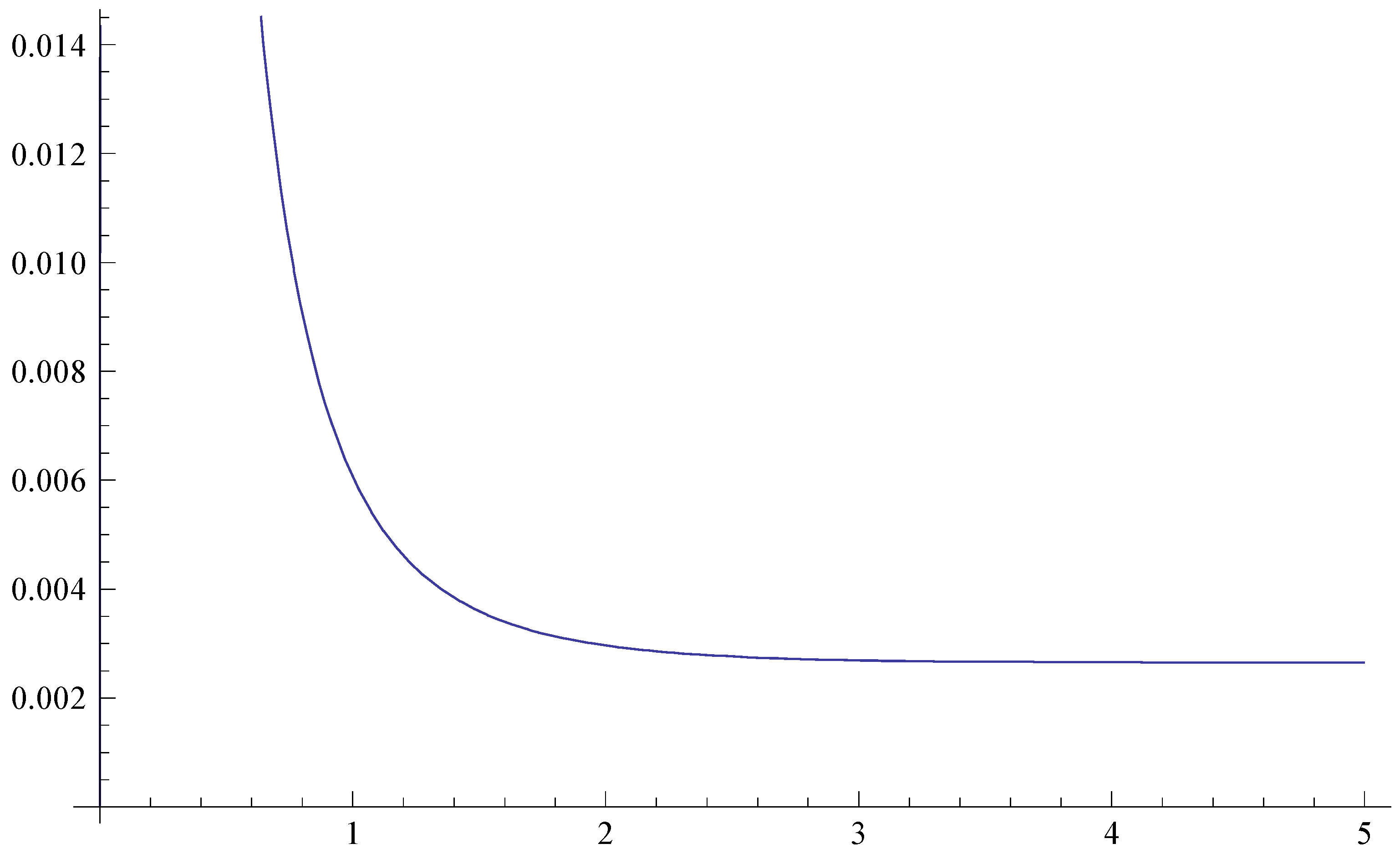
Disclaimer/Publisher’s Note: The statements, opinions and data contained in all publications are solely those of the individual author(s) and contributor(s) and not of MDPI and/or the editor(s). MDPI and/or the editor(s) disclaim responsibility for any injury to people or property resulting from any ideas, methods, instructions or products referred to in the content. |
© 2023 by the author. Licensee MDPI, Basel, Switzerland. This article is an open access article distributed under the terms and conditions of the Creative Commons Attribution (CC BY) license (https://creativecommons.org/licenses/by/4.0/).
Share and Cite
MDPI and ACS Style
Álvarez-Estrada, R.F. Approach to Equilibrium of Statistical Systems: Classical Particles and Quantum Fields Off-Equilibrium. Dynamics 2023, 3, 345-378. https://doi.org/10.3390/dynamics3020020
AMA Style
Álvarez-Estrada RF. Approach to Equilibrium of Statistical Systems: Classical Particles and Quantum Fields Off-Equilibrium. Dynamics. 2023; 3(2):345-378. https://doi.org/10.3390/dynamics3020020
Chicago/Turabian StyleÁlvarez-Estrada, Ramon F. 2023. "Approach to Equilibrium of Statistical Systems: Classical Particles and Quantum Fields Off-Equilibrium" Dynamics 3, no. 2: 345-378. https://doi.org/10.3390/dynamics3020020