
Dynamics of Fricke–Painlevé VI Surfaces


1
CNRS, Institut FEMTO-ST, Université de Franche-Comté, F-25044 Besançon, France
2
Quantum Gravity Research, Los Angeles, CA 90290, USA
*
Author to whom correspondence should be addressed.
Dynamics 2024, 4(1), 1-13; https://doi.org/10.3390/dynamics4010001
Submission received: 2 December 2023
/
Revised: 22 December 2023
/
Accepted: 29 December 2023
/
Published: 2 January 2024
Abstract
:The symmetries of a Riemann surface with n punctures are encoded in its fundamental group . Further structure may be described through representations (homomorphisms) of over a Lie group G as globalized by the character variety . Guided by our previous work in the context of topological quantum computing (TQC) and genetics, we specialize on the four-punctured Riemann sphere and the ‘space-time-spin’ group . In such a situation, possesses remarkable properties: (i) a representation is described by a three-dimensional cubic surface with three variables and four parameters; (ii) the automorphisms of the surface satisfy the dynamical (non-linear and transcendental) Painlevé VI equation (or ); and (iii) there exists a finite set of 1 (Cayley–Picard)+3 (continuous platonic)+45 (icosahedral) solutions of . In this paper, we feature the parametric representation of some solutions of : (a) solutions corresponding to algebraic surfaces such as the Klein quartic and (b) icosahedral solutions. Applications to the character variety of finitely generated groups encountered in TQC or DNA/RNA sequences are proposed.
1. Introduction
Free groups of rank and 3 have been found to be important in our earlier work about topological quantum computing (TQC) [1] and biology at the DNA/RNA genomic scale [2]. In the first context, one motivation is that an elementary link, the Hopf link made of two unknotted curves, may serve as a naive approach of TQC, corresponding to one qubit on either curve, as in [3]. Representation theory of the fundamental group over the group puts the punctured torus whose group is into focus. In the second context, at least in a first approximation, a finitely generated group defined from an appropriate DNA/RNA sequence turns out to be close to (for a sequence built from two distinct amino acids) or to (for a sequence built from three distinct amino acids). The character variety of such an group favors the topology of the triply punctured sphere (respectively, the quadruply punctured sphere ) whose fundamental groups are (respectively, ).
The interrelation between the free groups and becomes apparent in the exploration of fibrations associated with the Painlevé VI (or ) equation, a central focus of our inquiry. The discovery of the equation by R. Fuchs in 1905, during Einstein’s annus mirabilis, marked a pivotal moment in mathematical history. B. Gambier further highlighted its significance a year later, listing it as one of the six Painlevé transcendents [4]. These transcendents, ordinary second-order differential equations in the complex plane, defy expression in terms of familiar elementary or special functions, such as elliptic or hypergeometric functions.
The hallmark of Painlevé transcendents is the Painlevé property, denoting that the only movable singularities are poles. Recently, the attention has shifted towards unraveling the explicit algebraic solutions of , making it a hot topic with profound connections to algebraic geometry [5] and representation theory over the group [6]. It is worth recalling that , the special linear group of complex matrices with a determinant equal to 1, plays a crucial role in physics, particularly in the realm of symmetries and representations.
The realm of conformal field theory unveils another layer of connection, as the conformal group in two-dimensional space-time mirrors the isomorphism with [7]. This alignment assumes paramount importance in specific facets of string theory. The AdS/CFT correspondence further solidifies these connections, establishing a duality between a theory dwelling in anti-de-Sitter space (AdS) and a conformal field theory residing on its boundary [8]. Black-hole physics delves into the symmetrical nuances of , particularly in describing the isometries characterizing certain black hole solutions in general relativity, especially those with AdS asymptotic structures.
Turning our attention to the physical applications of , its profound interconnection with emerges prominently in the study of isomonodromic deformations and mathematical structures entwined with integrable systems [9,10]. Isomonodromic deformations, involving parameter variations in a second-order differential equation while preserving fixed monodromy properties, constitute a pivotal aspect of research. The associated monodromy matrices find their home within the confines of the group . The Garnier system, which encapsulates , manifests as a family of partial differential equations resonating across diverse physical contexts, including statistical mechanics [11].
In the intricate tapestry of string theory, solutions to unfurl within the study of moduli spaces of Riemann surfaces. Notably, the Painlevé equations emerge as reductions of partial differential equations, self-dual Yang–Mills equations [12], and within the intricate framework of random matrix theory [13]. takes center stage as it obediently materializes in combinations of conformal blocks within two-dimensional conformal field theory [14].
In Section 2, we embark on an exploration of the intricate mathematical landscape that establishes a profound connection between the topological intricacies of free groups and , isomonodromy deformations (deformations preserving monodromy), representations of fundamental groups, the enigmatic Painlevé VI equation, and the intriguing realm of Fricke–Painlevé surfaces. The initial manifestation of the link between and a complex surface is discerned in Jimbo’s seminal paper, specifically in ([15], Equation (1.6)).
The journey unfolds further as we trace the monodromy to its roots in the corresponding character variety, ultimately leading to the Jimbo–Fricke cubic, a concept expounded upon in works such as [16,17]. However, we introduce a more explicit conceptualization—the notion of a ‘Fricke–Painlevé VI surface’ (or simply Fricke–Painlevé surface) to precisely characterize the intriguing correspondence between a complex cubic surface and the dynamic equation . It is noteworthy that all algebraic solutions of have been meticulously documented [18].
Section 3 and Section 4 delve into the heart of the matter. In Section 3, our focus centers on parametric representations of algebraic solutions of and the drawing of log-log plots of some of them for the first time. Section 4 then extends our exploration to non-algebraic surfaces, providing a comprehensive view of the diverse landscape that traverses.
As the journey unfolds, Section 5 provides a reflective space where we deliberate on the diverse applications of Painlevé VI, particularly in the character varieties of finitely generated groups encountered in the realms of topological quantum computing (TQC) and genetics.
2. Materials and Methods
The concept of a flat connection on a fiber bundle takes shape, where the base B assumes the form of a three-punctured sphere, denoted as . For each point , a corresponding four-punctured sphere emerges. Let denote the fiber of M over the base point , and the monodromy action unfolds through the action of the fundamental group of the base on the fiber. This intricate dance is orchestrated by a homomorphism [5].
Now, let us offer a succinct overview of how the Painlevé VI equation is derived. Initiating the journey, a Fuchsian system of differential equations, boasting four singularities, takes the form:
where contains traceless matrices and poles at , . In this context, an isomonodromic deformation involves the movement of poles in the complex space and a variation in the entries of , all while conserving the conjugacy class of the corresponding monodromy representation. These deformations adhere to Schlesinger’s system:
Schlesinger’s equations not only preserve the adjoint orbit containing each but are also invariant under the conjugation of , , with representing the residue of at infinity.
For each point on the base B, we consider the set
which comprises conjugacy classes for representations of the fundamental group of the 4-punctured sphere with loops around the i-th puncture at the conjugacy classes , ( and . These representation spaces are two-dimensional and seamlessly fit into the fiber bundle .
For each , the space of conjugacy classes of representations for the fundamental group is the character variety
2.1. The Fricke–Painlevé VI Surface
Let the boundary components of be A, B, C, D, then . A representation of is the quadruple , , , with Taking the four boundary traces , , , and the three traces x, y, z of elements , , representing simple loops on , we obtain the character variety for ([6], Section 5.2), ([19], Section 2.1), ([20], Section 3B), ([21], Equation 1.9), ([22], Equation (39)), [18]
with , , and
From now, the 3-dimensional cubic surface with 3 variables and 4 parameters is called the Fricke–Painlevé surface due to the established correspondence between the automorphisms of such a surface and Painlevé VI equation.
Looking at the nonlinear monodromy of Painlevé VI, we obtain the relation between parameters a, b, c, d of and parameters , , of the Painlevé VI equation as ([21], Theorem 3), ([22], Section 4.2), ([18], Equation 13)
The Cayley’s Nodal Cubic Surface
The most famous Fricke–Painlevé surface follows from the fundamental group of the knot complement , where is the three sphere, is the group theoretical commutator and is the Hopf link. The character variety is given by the polynomial
where the notation is for the unique surface of the Fricke–Painlevé family, known as the Cayley nodal cubic surface, exhibiting four isolated singularities. A plot can be found in ([1], Figure 1).
3. Algebraic Solutions of Painlevé VI Equation Mapping to Algebraic Surfaces
Following the description of [24], an algebraic solution of equation should be specified by a polynomial equation with rational coefficients and a set of four parameters , .
More precisely, an algebraic solution of Painlevé VI is a compact (possibly singular) algebraic curve together with two rational functions y and t: providing a rational parametric representation ( such that (a) t is a Belyi map, with its branch locus being a subset of and (b) y solves for some parameters .
All algebraic solutions of have been classified in [18,25] building upon significant earlier contributions, including [26,27,28]. In [25], all algebraic solutions of , if not of the dihedral, tetrahedral or octahedral type, are refered to as isosahedral solutions as they can be derived from the finite monodromy subgroup of , where is the binary icosahedral group. Such solutions, governing the isomonodromic deformations of , have finite branching, with a number of branches ranging from 5 to 72.
Before the release of [25], the list of 45 exceptional solutions of was documented in the 2006 Cambridge slides by Philip Boalch [29]. Subsequently, for practical purposes, we adopt the solution numbering for as provided in [18].
Mapping an algebraic Fricke–Painlevé surface with integer parameters to an algebraic solution of Painlevé VI equation is one to one except for parameters (yielding three distinct solutions) and (yielding two distinct solutions) ([18], Table 4). In the first exceptional case the surface is a degree 3 del Pezzo surface of type (with one isolated singularity), while in the later case it is a degree 3 del Pezzo surface without a simple singularity. Detailed information about the 12 solutions () is provided in this section.
3.1. The Klein Solution
The Klein solution, corresponding to the Klein surface, is obtained with parameters [30], ([5], p. 26), ([18], solution 8). The parametric form of the solution is
It corresponds to the complex reflection group 24 in the Shephard–Todd list. The solution has seven branches and parameters . It is shown in Figure 1.
3.2. Solutions with Parameters
There are three solutions of corresponding to the algebraic surface . They are referred to as solution 3 (a tetrahedral solution with 6 branches), solution 21 with 12 branches and solution 42 with 36 branches in [18]. The surface is a degree 3 del Pezzo surface with an isolated singularity of type . It is depicted at the bottom of Figure 2.
The parametric form of the tetrahedral solution 3 is
The parametric forms for solutions 21 and 42 are found in [18]. The log-log plots of the solutions are given in Figure 2.
The parametric form of solution 3 has poles at and 3 which are evident as discontinuities in the log-log plot. For solution 21, there are poles at , 2, (i.e. and ). For solution 42, there are poles at and (i.e., and )
3.3. Solutions with Parameters
There are two solutions of corresponding to the algebraic surface . They are referred to as solution 20 (an octahedral solution with 12 branches) and solution 45 with 72 branches in [18]. The surface is of a degree 3 del Pezzo type devoid of an isolated singularity. It is depicted at the bottom of Figure 3.
The parametric form of the octahedral solution 20 is
3.4. The Great Dodecahedron Solution
The great dodecahedron solution, obtained with parameters ([18], solution 31), has the parametric form
The solution has 18 branches and parameters . A log-log plot for the modulus of solution 31 is shown in Figure 4 (Left) where the three poles at , and 1 are shown. The corresponding algebraic surface is a degree 3 del Pezzo of type .
3.5. Three Extra Solutions Leading to an Algebraic FRICKE-Painlevé Surface
There are three extra solutions corresponding to an algebraic Fricke–Painlevé surface. They correspond to the unique solutions with parameters (solution 1 with 5 branches), (solution 30 with 16 branches) and (solution 39 with 24 branches). The parametric expressions are in [18]. The log-log plots are found in Figure 5. The corresponding Fricke–Painlevé surfaces are degree 3 del Pezzo and devoid of isolated singularities.
4. Further Algebraic Solutions of Painlevé VI Equation
From now, we list further algebraic solutions of not related to an algebraic Frick—Painlevé surface.
4.1. The Icosahedral Solution 7
4.2. Dubrovin–Mazzocco Platonic Solutions
In [26], some platonic solutions of Painlevé VI equation are explored. These include the tetrahedral solution (solution III in [18] with 3 branches), the dihedral solution (solution IV in [18] with 4 branches), icosahedral solutions (solution 16 and 17 with 10 branches in [18]) and the great dodecahedron solution (solution 31 in [18]). These solutions are obtained for parameters , , , and , respectively. The great dodecahedron solution was previously mentioned in Section 3.4 and the parametric forms of other solutions are depicted in Figure 7. The explicit parametric forms can be found in the aforementioned papers.
4.3. Solutions Related to the Valentiner Group
The Valentiner group is the three-dimensional complex reflection group 27 with an order of 2160 in the Shephard–Todd list. Three solutions of are built upon this symmetry ([5], Theorem D). One of them is solution 39 described in Section 3.5. The other two are solutions 26 and 27 (with parameters and ), representing and 15 branches.
The solutions are plotted in Figure 8.
4.4. Two Extra Icosahedral Solutions
5. Discussion
5.1. Application to Character Varieties of Finitely Generated Groups
Our interest in Painlevé VI arises from our exploration of representations of finitely generated groups encountered in models of topological quantum computing (TQC) [1,17] and the investigation of DNA/RNA short sequences crucial in transcriptomics [2,31]. A model of TQC can commence with a link such as the Hopf link , whose character variety is the Cayley cubic surface given in (4). This surface is associated with the Picard solution of , as mentioned at the end of the introduction. Other links, such as or ([1], Figure 2), whose character varieties contain the Fricke–Painlevé surfaces for and 3 can be utilized. To these surfaces one can attach solution 30 of Painlevé VI (see Section 3.5 for the former case) and solutions 20 or 45 (see Section 3.3 for the latter case).
It has been observed that the truncated Groebner basis of four-letter groups encountered in the context of DNA/RNA sequences contains algebraic surfaces for and 4 as mentioned above, as well as the surface [2]. This surface corresponds to Fricke—Painlevé solution 31, with parameters , associated with the symmetry of the great dodecahedron (see Section 3.4). The surface with parameters is also part of the Groebner basis for four-letter groups. This reveals that many algebraic solutions of , the Picard solution for the Cayley cubic , solutions 20 and 45 associated with , solutions 3, 21 and 42 for parameters and the great dodecahedron solution 31 should play a role in genetics at the genome scale.
A Specific Example: (-Methyladenosine) Modifications
In the context of so-called epitranscriptomics, there are chemical modifications that control the metabolism of transcription of the genetic information. More than 170 types of RNA methylation processes have been discovered. The most common for eukaryotic organisms is the methylation of -methyladenosine () on some sites with a specific short sequence ( or G, , U or C); see e.g., [32,33,34]. In paper ([35], Table 2), we provide a group theoretical analysis of such sequences. For instance, the Groebner basis of three-nucleotide sequences and contain algebraic surfaces of type , or with , for the former sequence and , for the latter sequence. The exponent (*) in the surface refers to the type of A-D-E (simple) singularity of the surface ([35], Section 2.4). In our view, the occurrence of such a simple singularity in the character variety of a relevant sequence is associated with a potential disease. In addition, we observe that the aforementioned singularities do not belong to the list of singularities found in the context of Painlevé VI.
Let us now pass to the four-nucleotide sequence . This case is not investigated in much detail in ([35], Table 2). Below, we look at the the degree-2 Groebner basis associated with the character variety of group . The degree d-Groebner basis is the truncated Groebner basis obtained by ignoring polynomials of total degree larger than d. In our case, we obtain algebraic surfaces of the Fricke–Painlevé type.
For a four-nucleotide sequence, the degree-2 Groebner basis contains 14-dimensional surfaces of the form in (instead of 7-dimensional surfaces of the form in the case of a three-nucleotide sequence).
For the sequence , we find that, for parameters , contains decoupled surfaces , , and corresponding to the Picard solution of Painlevé VI. For parameters , contains decoupled surfaces , as well as the Fricke–Painlevé surfaces with parameters and variables and . For parameters , contains the decoupled Fricke—Painlevé surfaces with parameters and variables , , and . Then, for parameters , contains the decoupled Fricke-Painlevé surfaces with parameters and variables , the Fricke–Painlevé surface , as well as the Fricke–Painlevé surfaces with parameters and variables , and .
These explicit calculations confirm our hypothesis that some algebraic solutions of Painlevé VI may govern the dynamical transcription in genomics.
5.2. Perspectives
Isomonodromic deformation is a concept dating back to the nineteenth century, pioneered by P. Painlevé and subsequently studied by Fuchs, Schlesinger, Jimbo and numerous other scholars. This concept is underpinned by crucial mathematical properties of isomonodromy equations, including the Painlevé property, indicating that essential singularities remain fixed while poles may shift; transcendence, implying that solutions are non-classical; the existence of a symplectic structure, a twistor structure, and a Gauss–Manin connection. Isomonodromic deformation finds applications across various fields, such as random matrix theory, statistical physics, topological quantum field theory, nonlinear partial differential equations, Einstein field equations, and mirror symmetry.
While this paper primarily delves into the exploration of algebraic solutions of the Painlevé VI equation, it is noteworthy that the chaotic dynamics of has also received attention [36]. Further generalizations can be explored, as presented in [37]. In this latter paper, the role of is assumed by a differential equation governing the divergences in a formulation of renormalization in quantum field theory. The concept of a flat connection on a fiber bundle over the three-punctured sphere is significantly extended to a ‘flat equisingular bundle’ within a tensor category. The underlying symmetries are no longer discrete but are described by a motivic Galois group, also referred to as the `cosmic Galois group’, in line with ‘Cartier’s dream’ [38].
Author Contributions
Conceptualization, M.P. and K.I.; methodology, M.P. and D.C.; software, M.P.; validation, D.C.; formal analysis, M.P.; investigation, M.P. and D.C.; writing—original draft preparation, M.P.; writing—review and editing, M.P.; visualization, D.C.; supervision, M.P. and K.I.; project administration, M.P.; funding acquisition, K.I. All authors have read and agreed to the published version of the manuscript.
Funding
Funding was obtained from Quantum Gravity Research in Los Angeles, CA.
Institutional Review Board Statement
Not applicable.
Informed Consent Statement
Not applicable.
Data Availability Statement
Computational data are available from the authors.
Acknowledgments
The first author would like to acknowledge the contribution of the COST Action CA21169, supported by COST (European Cooperation in Science and Technology). He also acknowledges Philip Boalch for providing constructive feedback during the writing of version 2 of the paper.
Conflicts of Interest
The authors declare no conflict of interest.
References
- Planat, M.; Chester, D.; Amaral, M.M.; Irwin, K. Fricke topological qubits. Quant. Rep. 2022, 4, 523–532. [Google Scholar] [CrossRef]
- Planat, M.; Amaral, M.; Irwin, K. Algebraic morphology of DNA-RNA transcription and regulation. Symmetry 2023, 15, 770. [Google Scholar] [CrossRef]
- Asselmeyer-Maluga, T. Topological quantum computing and 3-manifolds. Quant. Rep. 2021, 3, 153. [Google Scholar] [CrossRef]
- Clarkson, P.A.; Joshi, N.; Mazzocco, M.; Nijhoff, F.W.; Noumi, M. One hundred years of PVI, the Fuchs—Painlevé equation. J. Phys. A Math. Gen. 2006, 39, EO1. [Google Scholar] [CrossRef]
- Boalch, P. From Klein to Painlevé via Fourier, Laplace and Jimbo. Proc. Lond. Math. Soc. 2005, 90, 167–208. [Google Scholar] [CrossRef]
- Goldman, W.M. Trace coordinates on Fricke spaces of some simple hyperbolic surfaces. Theor. Phys. 2009, 13, 611–684. [Google Scholar]
- Di Francesco, P.; Mathieu, P. Sénéchal, D. Conformal Field Theory; Graduate Texts in Contemporary Physics; Springer: New York, NY, USA, 1997. [Google Scholar]
- Biquard, O. AdS/CFT Correspondence: Einstein Metrics and Their Conformal Boundaries; EMS IRMA Lectures in Mathematics and Theoretical Physics; European Mathematical Society: Strasbourg, France, 2005; ISBN 978-3-03719-013-5. [Google Scholar]
- Isomonodromic Deformation. Available online: https://en.wikipedia.org/wiki/Isomonodromic_deformation (accessed on 1 August 2023).
- Gromak, V.I. The Painlevé Property: One Century Later; CRM Series in Mathematical Physics; Conte, R., Ed.; Springer: New York, NY, USA, 1999; pp. 687–734. [Google Scholar]
- Garnier Integrable System. Available online: https://en.wikipedia.org/wiki/Garnier_integrable_system (accessed on 1 December 2023).
- Mason, L.J.; Woodhouse, N.M.J. Integrability, Self-Duality, and Twistor Theory; London Mathematical Society Monographs; Oxford University Press: Oxford, UK, 1997. [Google Scholar]
- Forrester, P.J. Log Gases and Random Matrices; Princeton University Press: Princeton, NJ, USA, 2010. [Google Scholar]
- Gamayun, O.; Iorgov, N.; Lisovyy, O. Conformal field theory of Painlevé VI. J. High Energy Phys. 2012, 10, 38. [Google Scholar] [CrossRef]
- Jimbo, M. Monodromy problem and the boundary condition for some Painlevé equations. Publ. RIMS Kyoto Univ. 1982, 18, 1137. [Google Scholar] [CrossRef]
- Iorgov, N.; Lisovyy, O.; Tykhyyy, Y. Painlevé VI connection problem and monodromy of c = 1 conformal blocks. JHEP 2012, 10, 038. [Google Scholar] [CrossRef]
- Planat, M.; Amaral, M.M.; Fang, F.; Chester, D.; Aschheim, R.; Irwin, K. Character varieties and algebraic surfaces for the topology of quantum computing. Symmetry 2022, 14, 915. [Google Scholar] [CrossRef]
- Lisovyy, O.; Tykhyy, Y. Algebraic solutions of the sixth Painlevé equation. J. Geom. Phys. 2014, 85, 124–163. [Google Scholar] [CrossRef]
- Cantat, S. Bers and Hénon, Painlevé and Schrödinger. Duke Math. J. 2009, 149, 411–460. [Google Scholar] [CrossRef]
- Benedetto, R.L.; Goldman, W.M. The topology of the relative character varieties of a quadruply-punctured sphere. Exp. Math. 1999, 8, 85–103. [Google Scholar] [CrossRef]
- Iwasaki, K. An area-preserving action of the modular group on cubic surfaces and the Painlevé VI. Comm. Math. Phys. 2003, 242, 185–219. [Google Scholar] [CrossRef]
- Inaba, M.; Iwasaki, K.; Saito, M.H. Dynamics of the sixth Painlevé equation. arXiv 2005, arXiv:math.AG/0501007. [Google Scholar]
- Mazzocco, M. Picard and Chazy solutions to the Painlevé VI equation. Math. Ann. 2001, 321, 157–195. [Google Scholar] [CrossRef]
- Boalch, P. Towards a nonlinear Schwarz’s list. arXiv 2007, arXiv:0707.3375. [Google Scholar]
- Boalch, P. The fifty-two icosahedral solutions of Painlevé VI. J. Reine Angew. Math. 2006, 596, 183–214. [Google Scholar] [CrossRef]
- Dubrovin, B.; Mazzocco, M. Monodromy of certain Painlevé-VI transcendents and reflection groups. Invent. Math. 2000, 141, 55–147. [Google Scholar] [CrossRef]
- Hitchin, N. A lecture on the octahedron. Bull. Lond. Math. Soc. 2003, 35, 577–600. [Google Scholar] [CrossRef]
- Kitaev, L.V. Remarks towards the classification of (3)-transformations and algebraic solutions of the sixth Painlevé equation. Semin. Congr. Soc. Math. Fr. 2006, 14, 199–227. [Google Scholar]
- Boalch, P. Painlevé, Klein & the Icosahedron. Available online: https://webusers.imj-prg.fr/philip.boalch/abs/nlsl.html (accessed on 20 December 2023).
- Boalch, P. The Klein solution to Painlevé’s sixth equation. arXiv 2003, arXiv:math.AG/0308221. [Google Scholar]
- Planat, M.; Amaral, M.M.; Chester, D.; Irwin, K. SL(2, ℂ) scheme processsing of singularities in quantum computing and genetics. Axioms 2023, 12, 233. [Google Scholar] [CrossRef]
- Vissers, C.; Sinha, A.; Ming, G.L.; Song, H. The epitranscriptome in stem cell biology and neural development. Neurobiol. Dis 2020, 146, 105139. [Google Scholar] [CrossRef] [PubMed]
- Wang, S.; Lv, W.; Li, T.; Zhang, S.; Wang, H.; Li, X.; Wang, L.; Ma, D.; Zang, Y.; Shen, J.; et al. Dynamic regulation and functions of mRNA m6A modification. Cancer Cell Int. 2022, 22, 48. [Google Scholar] [CrossRef] [PubMed]
- Widagdo, J.; Wong, J.J.L.; Anggono, V. The m6A-epitranscriptome in brain plasticity, learning and memory. Semin. Cell Dev. Biol. 2022, 125, 110–121. [Google Scholar] [CrossRef] [PubMed]
- Planat, M.; Amaral, M.M.; Fang, F.; Chester, D.; Aschheim, R. Irwin, K. Group theory of messenger RNA metabolism and disease. Gene Expr. 2023, in press. [Google Scholar] [CrossRef]
- Cantat, S.; Loray, F. Holomorphic dynamics, Painlevé VI equation and character varieties. arXiv 2007, arXiv:1207.0154. [Google Scholar]
- Connes, A.; Marcolli, M. Quantum fieds and motives. J. Geom. Phys. 2006, 56, 55–85. [Google Scholar] [CrossRef]
- Cartier, P. A mad day’s work: From Grothendieck to Connes and Kontsevich. The evolution of concepts of space and symmetry. Bull. Amer. Math. Soc. 2001, 38, 389–408. [Google Scholar] [CrossRef]
Figure 1.
(Left): Parametric plot for the modulus of Klein solution of (solution 8 of ([18], p. 157)); the discontinuities of the plot correspond to the four poles. (Right): the corresponding cubic surface .
Figure 1.
(Left): Parametric plot for the modulus of Klein solution of (solution 8 of ([18], p. 157)); the discontinuities of the plot correspond to the four poles. (Right): the corresponding cubic surface .
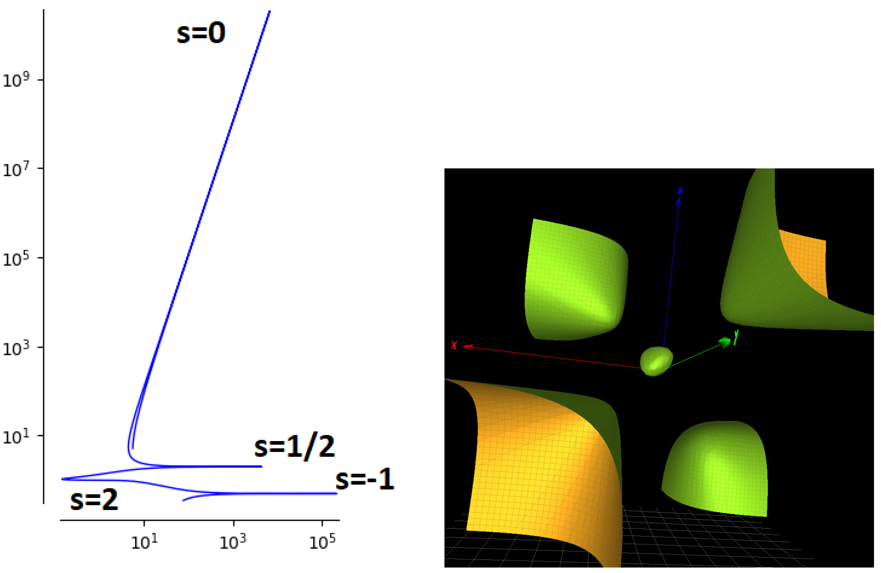
Figure 2.
Solutions related to the algebraic surface are indexed in [18]. (Upper left): the tetrahedral solution 3. (Upper right): solution 21. (Middle): modulus of solution 42. (Lower): the corresponding algebraic surface. It is a degree 3 del Pezzo surface of the type.
Figure 2.
Solutions related to the algebraic surface are indexed in [18]. (Upper left): the tetrahedral solution 3. (Upper right): solution 21. (Middle): modulus of solution 42. (Lower): the corresponding algebraic surface. It is a degree 3 del Pezzo surface of the type.

Figure 3.
Solutions related to the algebraic surface are indexed in [18]. (Upper left): the modulus of the octahedral solution 20. (Upper right): the modulus of solution 45. (Lower): the corresponding algebraic surface.
Figure 3.
Solutions related to the algebraic surface are indexed in [18]. (Upper left): the modulus of the octahedral solution 20. (Upper right): the modulus of solution 45. (Lower): the corresponding algebraic surface.

Figure 4.
(Left): Parametric plot for the modulus of the great dodecahedron solution of (solution 31 of ([18], p. 157)); the three poles are identified. (Right): the corresponding cubic surface is a degree 3 del Pezzo surface of type that is with three isolated singularities).
Figure 4.
(Left): Parametric plot for the modulus of the great dodecahedron solution of (solution 31 of ([18], p. 157)); the three poles are identified. (Right): the corresponding cubic surface is a degree 3 del Pezzo surface of type that is with three isolated singularities).

Figure 5.
Parametric plots for the modulus of solutions 1 (with 5 branches: Fricke–Painlevé form ), 30 (an octahedral solution with 16 branches: Fricke–Painlevé form ) and 39 (a Valentiner solution with 24 branches: Fricke–Painlevé form .)
Figure 5.
Parametric plots for the modulus of solutions 1 (with 5 branches: Fricke–Painlevé form ), 30 (an octahedral solution with 16 branches: Fricke–Painlevé form ) and 39 (a Valentiner solution with 24 branches: Fricke–Painlevé form .)
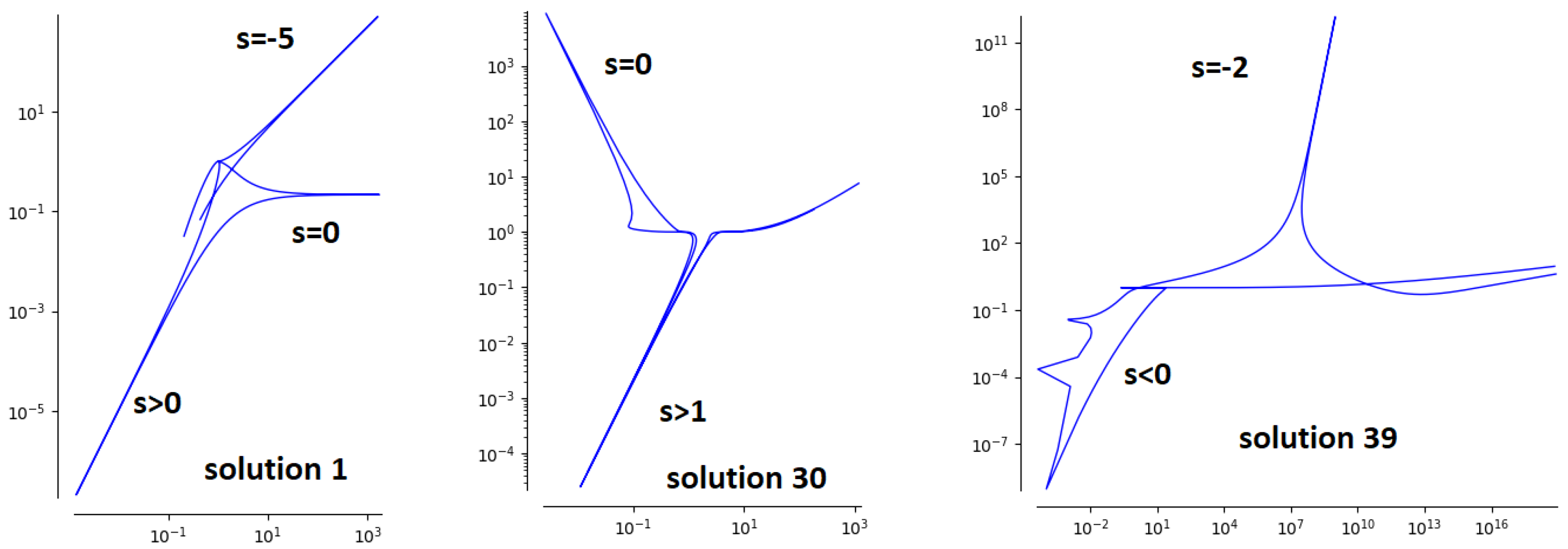
Figure 6.
(Left): Parametric plot of an icosahedral solution of (solution 7 of ([18], p. 157)); the discontinuities of the plot correspond to the poles. (Right): the corresponding cubic surface.
Figure 6.
(Left): Parametric plot of an icosahedral solution of (solution 7 of ([18], p. 157)); the discontinuities of the plot correspond to the poles. (Right): the corresponding cubic surface.

Figure 7.
Parametric plots for the modulus of solutions III (the tetrahedral solution), IV (the dihedral solution), solutions 16 and 17 (icosahedral solutions) as first described in [26]. For the later two solutions, we find poles located at irrational values , , and .
Figure 7.
Parametric plots for the modulus of solutions III (the tetrahedral solution), IV (the dihedral solution), solutions 16 and 17 (icosahedral solutions) as first described in [26]. For the later two solutions, we find poles located at irrational values , , and .

Figure 8.
Parametric plots for the modulus of solutions 26 and 27 that are related to the Valentiner group.
Figure 8.
Parametric plots for the modulus of solutions 26 and 27 that are related to the Valentiner group.

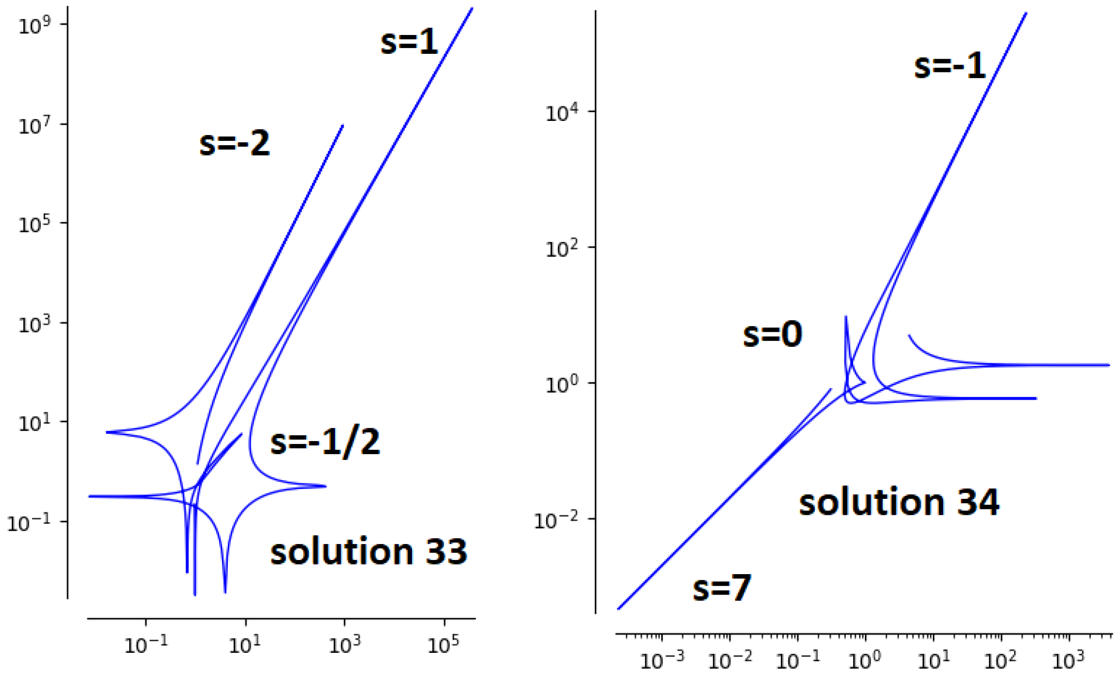
Figure 9.
Parametric plots for the modulus of solutions 33 and 34.
Disclaimer/Publisher’s Note: The statements, opinions and data contained in all publications are solely those of the individual author(s) and contributor(s) and not of MDPI and/or the editor(s). MDPI and/or the editor(s) disclaim responsibility for any injury to people or property resulting from any ideas, methods, instructions or products referred to in the content. |
© 2024 by the authors. Licensee MDPI, Basel, Switzerland. This article is an open access article distributed under the terms and conditions of the Creative Commons Attribution (CC BY) license (https://creativecommons.org/licenses/by/4.0/).
Share and Cite
MDPI and ACS Style
Planat, M.; Chester, D.; Irwin, K. Dynamics of Fricke–Painlevé VI Surfaces. Dynamics 2024, 4, 1-13. https://doi.org/10.3390/dynamics4010001
AMA Style
Planat M, Chester D, Irwin K. Dynamics of Fricke–Painlevé VI Surfaces. Dynamics. 2024; 4(1):1-13. https://doi.org/10.3390/dynamics4010001
Chicago/Turabian StylePlanat, Michel, David Chester, and Klee Irwin. 2024. "Dynamics of Fricke–Painlevé VI Surfaces" Dynamics 4, no. 1: 1-13. https://doi.org/10.3390/dynamics4010001