An Enhanced Mechanism for Fault Tolerance in Agricultural Wireless Sensor Networks

Abstract

Fault tolerance is a critical aspect for any wireless sensor network (WSN), which can be defined in plain terms as the quality of being dependable or performing consistently well. In other words, it may be described as the effectiveness of fault tolerance in the event of crucial component failures in the network. As a WSN is composed of sensors with constrained energy resources, network disconnections and faults may occur because of a power failure or exhaustion of the battery. When such a network is used for precision agriculture, which needs periodic and timely readings from the agricultural field, necessary measures are needed to handle the effects of such faults in the network. As climate change is affecting many parts of the globe, WSN-based precision agriculture could provide timely and early warnings to the farmers about unpredictable weather events and they could take the necessary measures to save their crops or to lessen the potential damage. Considering this as a critical application area, in this paper, we propose a fault-tolerant scheme for WSNs deployed for precision agriculture. Along with the description of our mechanism, we provide a theoretical operational model, simulation, analysis, and a formal verification using the UPPAAL model checker.

1. Introduction

Nowadays, wireless sensor networks (WSNs) have become widely used in many aspects of our daily life such as in healthcare [1,2,3], including for remote patient monitoring, medication adherence monitoring, and sleep monitoring; in smart cities [4,5] for smart transportation and energy management; and in agriculture [6,7,8], such as for weather monitoring, environmental monitoring, and livestock monitoring, and so on. A WSN is basically an infrastructure comprised of sensing, computing, and communication elements (i.e., micro-sensors) that gives an administrator the ability to monitor, observe, and react to events and phenomena in a specified environment [9,10,11,12]. WSNs have the characteristics of convenient deployment, low cost, and high precision, which make them suitable for agricultural information monitoring and transmission [13,14]. Over the last few years, sensors and WSNs have emerged at an extraordinary rate [15,16,17]. A key reason for this is the ability of WSNs to perform real-time data monitoring and reporting. This capability enables the acquisition of multisource environmental and crop state data in the case of precision agriculture [18,19,20,21,22,23].

To date, several agriculture precision applications based on WSN [13,14,24,25,26,27] have been proposed to keep farmers informed about their farm field conditions with valuable data such as temperature, humidity, wind speed, rainfall, and so on. In fact, with climate change, we are currently witnessing random weather events and unexpected weather conditions in various parts of the world. Hence, if accurate information on farm fields and agricultural activities can be collected in time, it can be used to significantly reduce losses and damage to crops and increase the overall agricultural productivity. In this scenario, WSNs can be a panacea for precision agriculture. However, like any other system, WSNs also suffer from malfunctions and failures. An essential obstacle in WSN design lies in meeting diverse application demands (such as lifetime, throughput, and reliability) within the constraints of limited energy, computation, and storage capacity of sensor nodes. In fact, deployment in unattended or hostile environments increases the susceptibility of sensor nodes to failures compared to other systems. Faults in WSN can be classified into hardware and software faults. Hardware faults are due to physical defects, energy depletion, environmental interference, or insufficient storage. The cited factors can lead to a transient or permanent crash and can result in software failures. Software faults are generally caused by a limited computational capacity and sometimes by intruder attacks [28,29,30]. The failure of any WSN component can lead to sensor network partitioning, where the nodes become isolated and disconnected from the network, resulting in reduced availability and potential failure of the WSN as a whole.

When we take various aspects of WSNs into consideration, we find that a major issue is the energy consumption of WSNs. As we know, such wireless devices (i.e., sensors and actuators) run on batteries and have a limited amount of energy. So, when a node in the path that transmits packets from a source to a destination dies, the transiting packets will be lost because of the unsuccessful transmission. In such cases, the network must be able to rectify the fault of the node and identify an effective solution for better transmission and continued operation.

Fault tolerance is an essential attribute of a WSN for precision agriculture. A WSN used for precision agriculture must satisfy the dependability properties of safety and liveness. In this paper, considering the setting of precision agriculture, a fault tolerance scheme is introduced. The aim was to detect crashed nodes and recover from the node failure to allow for continued data transmission, which could therefore eventually extend the network lifetime. A simulation model with fault injection and performance evaluation using queries is also provided to validate our approach.

The rest of the paper is organized as follows: Section 2 presents some relevant works. Then, the WSN topology used in this paper is explored in Section 3. In Section 4, the theory for our WSN fault-tolerant model is provided. In Section 5, a fault detection and recovery scheme for our WSN is proposed. Then, a formal conception and verification of the proposed scheme is provided in Section 6 using the UPPAAL model checker. In Section 7, complexity estimation is introduced and a comparative analysis against some recent works is provided. Finally, Section 8 concludes the paper with future research direction.

2. Related Work

In this section, we will summarize some of the key research papers that have motivated us to develop our mechanism. A wide variety of works have addressed various aspects in this domain and we have obtained critical information from each of these works.

Shyama and Pillai explored fault tolerance, fault recovery, fault prevention, and fault detection techniques in WSNs in [31]. In [32], Sheth and Jani proposed a fault-tolerant technique for the detection of faults at the sensor node level where, depending on the group detection method, each node can be monitored by several other nodes. The fault detection is performed using a detection tree in which a hierarchy is defined for the identification of failed nodes. The proposed formula was analyzed according to a probabilistic approach. Shankar et al. introduced a fault tolerance model in [33] to improve the WSN lifetime by reducing the energy consumption over the network nodes; to do this, a pollination algorithm for was used. MATLAB 2018a has been utilized as a simulation environment for the anticipated model. In [34], in order to achieve a balance between the two metrics of energy consumption and packet loss, Al-Hawri et al. proposed a data dissemination protocol based on probabilistic network coding. This was carried out by using a subset of the network nodes in a directed acyclic graph.

There are also several fault-tolerant routing protocols proposed in the existing literature. A selected few are summarized here. Shyama et al. developed swarm genetic optimization (FTGSO) for fault-tolerant routing path identification in [35]. In this work, the selection of the Cluster Head (CH) was carried out using several metrics such as residual energy, coverage, communication cost, and proximity. The proposed model was compared with other optimization algorithms and the evaluation results verified the superior performance of the proposed scheme. In [36], Hallafi et al. proposed a method that aimed to detect network holes. In this method, the network is geographically cellulated, and a cell agent is selected for each cell. Then, the coverage of nodes within each cell is calculated. After that, it is possible to detect holes in the network cells. Finally, the holes are recovered using mobile nodes using the grasshopper optimization algorithm. In [37], Papi and Barati introduced a method to maintain coverage in WSNs. The proposed method is composed of two phases: the first phase aims to detecting holes through a simple distributed method by which each node explores whether there are holes around it or not. In the second phase of the proposed method, the holes are covered using mobile nodes.

A regression-based fault detection and tolerance strategy for WSNs was introduced in [38] by Swain et al. The proposed strategy diagnoses the different types of faulty nodes with the help of the data sensed by the fault-free neighbors. In [39], Goyal et al. proposed a fault detection and recovery technique (FDRT) for a cluster-based network. Essentially, the principle is to choose a Cluster Head (CH) and to select a Backup Cluster Head (BCH) using the fuzzy logic technique. In the case of failure of the CH, the BCH will continue the task of the failed CH. In [40], Wu et al. provided a potential game and the cut vertex detection mechanism, which are utilized to establish a fault-tolerant topology which consists of a set of single hop clusters. The main objective was to reduce the energy consumption of the network. Therefore, an algorithm based on a double price function was designed.

3. WSN Topology

In this paper, a WSN for precision agriculture was used and a hierarchical topology was adopted for this WSN. It is composed of a set of balanced clusters. Each cluster is formed by a set of sensor nodes managed by a Cluster Head (CH). The sensor nodes collect and transmit data to the CHs in one hop. The CHs receive and process the data transmitted by the nodes, then transmit the processed data to the Base Station (BS) with a single hop. In general, clustering [41] has been proven to be an effective energy-saving method in WSNs.

3.1. The Structure of the WSN

In this sub-section, we describe the structure of the WSN along with its key components and assumptions (for our model).

Sensor Nodes: These nodes are deployed by the farmers in the agriculture field at specific places; hence, each node has specific coordinates. Each node has a unique ID (identification number). The main role of the sensor node is to collect environmental data (e.g., temperature and humidity) in the field of interest and then transmit the collected data with its proper ID to the CH with a single hop.

Cluster Head (CH): It is a particular sensor node with relatively higher energy resource, and with a better computing and storage capacity. There are several CHs in the WSN. A CH has deterministic coordinates; it acts as an interface for communication between its members and the Base Station. The CH manages the communications within its cluster according to the Time Division Multiple Access (TDMA) protocol [42]. The CH must perform an aggregation processing of the received data in order to minimize the number of messages transmitted to the Base Station. The communication between the CH and the Base Station is performed with a single hop.

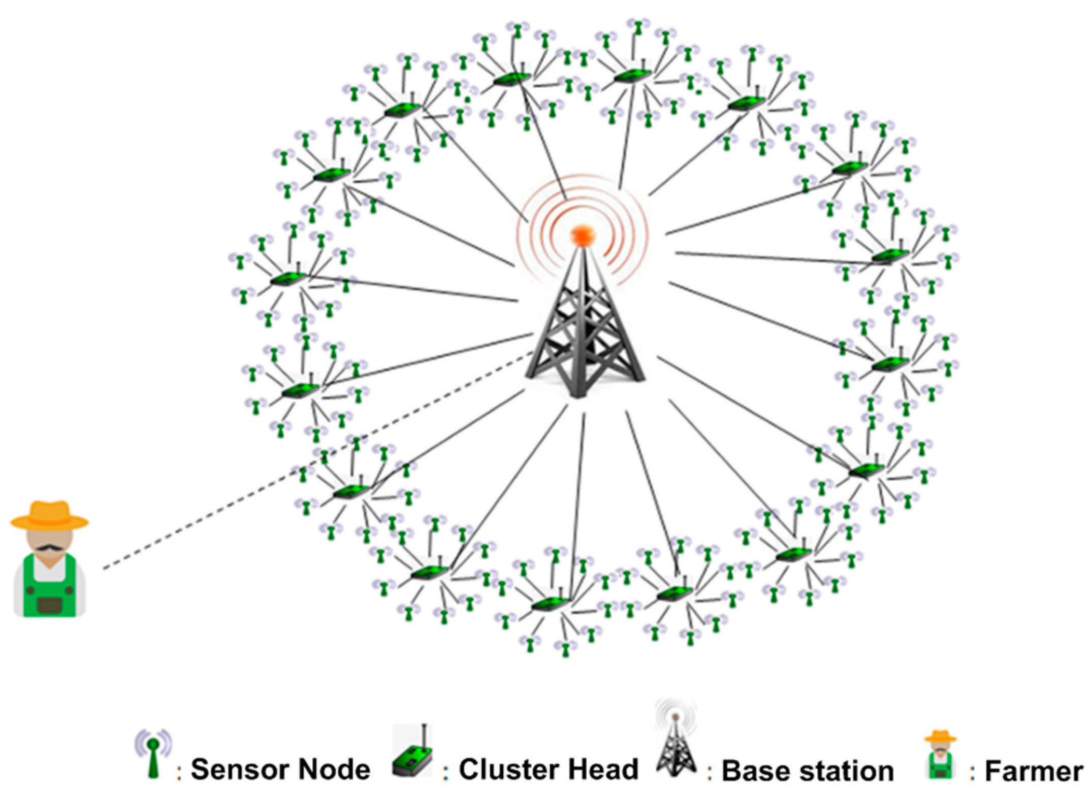
Base Station (BS): It manages the entire network; it receives the data sent by different CHs and retransmits data to the final user. This transmission can be performed via the Internet while taking the advantage of the Internet of Things (IoT) environment. In other words, crop management, monitoring, and control can be carried out remotely via the Internet using a PC or a smartphone. In fact, the user knows the geographical map of all sensor locations, which allows them to intervene to possibly replace a defective sensor or a depleted battery. In order to make the nodes equidistant from their CH in our model, we used the deployment strategy that divides the monitored field into circular regions where the CHs are located at the center of each circle. The BS is also placed in the center of crop field (see Figure 1).

As illustrated in Figure 1, a simple clustering mechanism was applied, in which, the agricultural field is divided into several circular zones with the CHs located in the center of the circles and all the clusters contain the same number of sensor nodes. This is possible to implement for an agricultural field as the farmer can physically access the land. Therefore, each sensor node has the same distance from the associated CH as any other sensor node in the same cluster. We can say that the clustering topology used in our model guarantees network scalability and is an effective energy-saving technique (by the nature of the deployment).

3.2. WSN Routing and Data Transmission

In our scheme, the sensor nodes are associated with the nearest CHs, where the CHs announce their coverage with their identification to all members of the cluster. After that, each CH sends a scheduling TDMA to all cluster members; in this way, it allows all sensor nodes to allocate a time slot for the transfer of their data. In this part, the routing mechanisms between the WSN devices are explored.

3.2.1. Routing Mechanism for Sensor Nodes and the CH

The routing mechanism is divided into two main stages. The first step is data communication between sensor nodes and the CH (see Figure 2), while the second step consists of data aggregation and data transmission from the CHs to the BS.

After the deployment of the network devices on the agricultural field, the group leader (e.g., CHs) broadcasts an announcement with its identification number (ID) over the cluster. When the sensor nodes receive the CH’s announcement, they reply with a join request to their leader. After that, the CH sends the TDMA scheduling, allowing each node to have a time slot for the transmission of its data. Once the node receives its TDMA, it enters a passive state (e.g., sleeping state) while waiting for the data request sent by the leader CH. Once the cluster establishment is completed, the data transfer can take place.

When the time slot arrives, the CH sends a data request to the associated sensor. At the moment of receiving the data request, the sensor node enters the active state (e.g., awake state) and it collects information from its environment and sends it to CH. After that, it re-enters the passive state. In this way, the node saves energy and therefore, extends its lifetime. After having received all the environmental information from the sensor nodes, the leader CH can aggregate the data and put them into a single packet in order to send it to the BS. The cluster construction process is presented in Algorithm 1.

Algorithm 1. Cluster Construction in a WSN

Input: Wireless sensor network

Output: WSN hierarchical structure based on clusters

1. Cluster Head initialization () 2.    Broadcast the cluster ID (${CH}_{ID}$) over the cluster; 3.    For loop = 1 to m sensor 4.          If CH receives the join request from ${node}_{id}$ then 5.             Send TDMA to ${node}_{id}$; 6.             Thread ${Node}_{id}$ in the node file; 7.          End If 8.    End loop 9.      Initiate Node_TimeOut as node data reception deadline; 10. End Cluster Head initialization()

11. Sensor node initialization() 12.   If the sensor node receives the ${CH}_{ID}$ from the CH then 13.       Send a join request with the node ID to the CH; 14.       If the sensor node receives the TDMA from the CH then 15.          Go the passive state() //Waiting for a data request from the CH; 16.       End If 17.   End If 18. End Sensor node initialization()

3.2.2. Routing Mechanism for CHs and BS

After building the cluster group, the CH first sends a join request containing its ID to the unique BS. After the request is received by the BS, it will answer with a TDMA in order to give the sender CH a time slot for exchanging data. Through this, the CH establishes a route with its associated BS (see Figure 3). When the time slot arrives for the CH, the BS sends a data request to the CH. The CH then receives the request, and in turn, transfers the aggregated data collected from sensor nodes to the BS. The routing protocol initialization between the CHs and BS is detailed in the Algorithm 2.

Algorithm 2. CH and Base Station communication initialization.

Input: Wireless sensor network

Output: WSN hierarchy structure

1. Base station initialization() 2. Broadcast BS ID over the network; 3.    For loop = 1 to m CH 4.     If Base station receives a Join Request from a ${CH}_{ID}$ then 5.         Send $TDMA$ to the CH ${CH}_{ID}$; 6.         Thread ${CH}_{ID}$ in CHs file; 7.     End If 8.    End For 9.    Initiate CH_TimeOut; 10. End Base station initialization()

4. Theoretical Model for Our Fault-Tolerant WSN

In this section, we present the theory behind our fault-tolerant wireless sensor network.

Definition 1.

A node is defined as a tuple $n(ID, p)$, such that $ID$ is the node identity and p is the energy level, $p\in [p_{Min}, p_{Max}]$.

Definition 2.

A cluster is defined as a tuple $C=\{N, L, T, CH\}$, such that

N: the set of nodes $\left\{n^0, n^1, \dots ,n^m\right\}$;

L: the set of communication links $\left\{l_0,l_1, \dots ,l_n\right\}$ between the sensor nodes and the CH;

T: a set of transitions t, and each transition is a tuple of the form $t=\left(n^i, l^i,p^i, d^i,CH\right), (i=0\dots m)$, where

• $n^i$: the sensor node;
• $l^i$: the communication link associated with the transition;
• $p^i: \in [p_{Min}, p_{Max}]$, the transmit power of the sender node;
• $d^i$: the set of transmitted data;
• $CH$: the Cluster Head.

Definition 3.

A fault-tolerant cluster $C=\{N, L, T, CH\}$ is a cluster that contains a primary CH and a backup CH, ${FT}_C=\left({Primary}_{CH}, {Backup}_{CH}, N, L,T\right)$, such that

-

${Primary}_{CH}\left({ID}_{pr}, p_r\right)$ is the main $CH$ in the cluster group. It is characterized by its proper ${ID}_{pr}$, and its energy level $p_r$.

-

${Backup}_{CH}({ID}_{Bk}, p_{Bk})$ is the backup $CH$; it has an ${ID}_{Bk}$ and an energy level such that $p_{Bk}=p_r$.

Here, $L$ is the set of communication links $L={\cup }_{i=1}^m{\cup }_{j=1}^m{l}_i{l^{\prime }}_j;$ there are two types of communication links: the communication links between the sensor nodes and the ${Primary}_{CH}(l_1,l_2, \dots , l_m)$ and those between the sensor nodes and the ${Backup}_{CH} ({l^{\prime }}_1,{l^{\prime }}_2, \dots , {l^{\prime }}_m)$.

Lemma 1.

A fault-tolerant cluster, ${FT}_C=\left({Primary}_{CH}, {Backup}_{CH}, N, L,T\right)$, is able to ensure the safety and liveness of the cluster group.

Proof. 

In order to prove Lemma 1, we will use reductio ad absurdum. Let us consider the following scenarios. Let $C=\left\{N, L, T, CH\right\}$ be a non-fault-tolerant cluster, which has no backup CH.

At moment $t$, the initial power level of the CH is $p=P_{Max}$.

At moment $t\prime$, the CH receives data from all the sensor nodes in the cluster (i.e., each data transaction needs $\delta power$); at that time, $p=P_{Max}-m\delta$.

At moment $t^{″}$, the CH aggregates and transmits data to the BS that needs $\epsilon energy$; thus, $p=P_{Max}-(m\times \delta +\epsilon )$.

At moment $t^{‴}$, the CH repeats the tasks $\theta times$ while:

$:P_{Min}\le p(\theta \times \left(m\times \delta +\epsilon \right))\le P_{Max}$.

After $\theta$ times, the CH exhausts its energy: $p\le P_{Min}$. At that time, the CH has completely stopped functioning, the field data of the $m$ sensor nodes have been lost and the sensor group is currently disconnected from the rest of the network. In fact, this disconnection could lead to significant damage in the agricultural field. Hence, we conclude that the cluster is neither safe nor live.

However, in the case of using a backup Cluster Head, at moment $t^{‴}$, the failure of the primary CH will be detected and the backup CH will immediately take the role. □

Definition 4.

A Base Station is defined as a tuple $BS({ID}_{BS}, \mu )$, such that $ID$ is the Base Station identity and $\mu$ is the residual energy of the BS, $\mu \in [{\mu }^{Max},{\mu }^{Min}]$.

Definition 5.

A fault-tolerant Base Station BS, ${FT}_{BS}$ = $({Primary}_{BS}, {Backup}_{BS})$, is composed of a primary Base Station (i.e., ${Primary}_{BS}$) and a backup Base Station (i.e., ${Primary}_{BS}$). Here, ${Primary}_{BS}\left({ID}_{PBS}, {\mu }_{pr}\right)$ is the main $BS$ in the WSN whereas ${Backup}_{CH}({ID}_{BBS}, {\mu }_{BBS})$ is the backup $BS$.

Lemma 2.

A fault-tolerant BS, ${FT}_{BS}$ = $({Primary}_{BS}, {Backup}_{BS})$, is able to offer safe and live data transmission to the end user.

Proof. 

Let us consider a WSN composed of a set of clusters and one non-fault-tolerant Base Station with a residual energy, $\mu \in [{\mu }^{Max},{\mu }^{Min}]$. Let us consider the following scenarios:

At moment $t$, the BS receives data from the set of ${CH}_{i=1\dots n}$. If we assume that a single data reception consumes $\sigma$, then, $\mu =\mu -(n\times \sigma )$, ${\mu }^{Min}\le \mu \le {\mu }^{Max}$.

At moment $t^{\prime }(t^{\prime }>t)$, the BS aggregates and transmits data to the end user. If we assume that this task needs $\phi$ amounts of energy, then the residual energy is $\mu -(n\times \sigma +\phi )$, ${\mu }^{Min}\le \mu \le {\mu }^{Max}$.

At moment $t″(t″>t^{\prime }>t)$, after repeating the process $\omega$ times, $\mu =\mu -\omega \times \left(n\times \sigma +\phi \right)\le {\mu }^{Min}$; at this time, the BS has exhausted its energy and then stops operating. The $CH$’s data will then be lost and the entire WSN will become disconnected from the external world. Therefore, safety and liveness are both violated in the WSN system.

On the other hand, a backup BS can come to the rescue of the situation at moment $t″$ (i.e., after the detection of failure of primary BS).

We can conclude that a fault-tolerant BS can ensure safe and live data transmission in the WSN. □

Definition 6.

A WSN system $wsn=\left( C, L, T, BS\right)$ is defined by a composition of set of clusters that rely on a set of connection links and one Base Station such that

• $C=\left\{C_0\dots C_n\right\}$ is the set of clusters;
• $L=\{l_0,l_1,l_2,\dots ,l_n\}$ is the set of connection links, such that $\{\forall l_{i\in \left(1..n\right)},l_{i}relies{C}_{i}toBS\}$;
• $T$ is a set of transitions $\tau$, and each transition is a tuple of the form $\tau =\left({CH}_i, l_i,p_i, d_i,BS\right) (i=1..n)$, where
  • ${CH}_i$ is the leader in cluster $i$;
  • $l_i\in \gamma$ is the communication link between the ${CH}_i$ and the Base Station;
  • $p_i\in [p_{Min},p_{Max}]$ is the transmission power consumed by the ${CH}_i$;
  • $d_i$ is the transmitted data from ${CH}_i$ to the Base Station;
  • $BS$ is the unique Base Station.

Definition 7.

A fault-tolerant ${FT}_{wsn}=\left( {FT}_c, L, T, {FT}_{BS} \right)$ is composed of s sets of fault-tolerant clusters, ${FT}_C^{i=1..n}$, and a set of connectors, L, relies on a fault-tolerant Base Station ${FT}_{BS}$.

Theorem 1.

A fault-tolerant ${FT}_{wsn}=\left( {FT}_c, L, T, {FT}_{BS} \right)$ WSN is able to ensure safe and live agricultural data transmission.

Proof. 

Let us consider a WSN composed of a set of fault-tolerant clusters presented by their CHs (${FT}_{CH1,}, { FT}_{CH2}, { FT}_{CH3}$) and one non-fault Base Station (BS). Let us discuss the first scenario.

During time $[t_0-t_1$], the three clusters collect the environmental information and transmit the data to the Base Station.

At moment $t_2$, the BS transmits data to the end user.

During time [$t_2-t_3$], the Cluster Heads ${FT}_{CH1} \mathrm{a}\mathrm{n}\mathrm{d} { FT}_{CH2}$ deplete their energy, and only ${FT}_{CH3}$ collects information and sends data to the BS.

At moment $t_4$, the backup Cluster Heads, ${FT}_{BCH1}$ and ${FT}_{BCH2}$, take over the role and transmit the collected data to the BS.

At moment $t_5$, the BS aggregates and transmits data to the end user, and Cluster Head ${FT}_{CH3}$ exhausts its energy and it will be replaced by the its backup: ${FT}_{BCH3}$.

During time $[t_6-t_7]$, the backup Cluster Heads ${FT}_{BCH1}$, ${FT}_{BCH2}$, and ${FT}_{BCH3}$ collect, aggregate, and transmit data to the BS. At that moment, the BS depletes its energy and stops operating. Unfortunately, cluster’s data will be lost and the WSN service will be interrupted until the Base Station is repaired. Hence, safety and liveness are violated in such a scenario.

Let us now consider a second scenario, in which a WSN is composed of a set of non-fault-tolerant clusters presented by the Cluster Heads ($CH1, CH2, CH3$) and one fault-tolerant ${FT}_{BS}$.

During time $[t_1-t_2]$, the set of clusters sense the field information and transmit data to the BS.

At time $t_3,$ the BS receives, aggregates, and sends data to the end user.

During the time $[t_4-t_5]$, Cluster Head $CH1$ stops functioning due to energy depletion, causing cluster isolation, but $CH2$ and $CH3$ keep operating by sending data to the BS.

At moment $t_6$, ${FT}_{BS}$ receives and transmits data to the end user.

During time $[t_7-t_8]$, Cluster Head $CH2$ depletes its energy and then stops; therefore, only one Cluster Head ($CH3$) collects and transmits the data packet to the BS.

At moment $t_9$, the Base Station exhausts its residual energy and is immediately replaced by its backup: ${FT}_{BBS}$. The latter entity continues operating by receiving the collected data and transmitting the data packets to the end user.

At moment $t_{10}$, Cluster Head $CH3$ exceeds its energy and hence, stops operating as $CH1 \mathrm{and} CH2$. At that time, all clusters will be disconnected from the entire WSN and all environmental data will be lost. Therefore, safety and liveness have been violated in this scenario.

Hence, we can conclude that to construct a fault-tolerant WSN, it has to be composed of a set of fault-tolerant clusters and a fault-tolerant Base Station. □

5. Fault-Tolerant Scheme for WSN in Precision Agriculture

In this kind of WSN system, the failure of the BS could completely isolate the WSN from the final user (e.g., the farmer) and cause a complete loss of the collected data. Also, the failure of a CH will deprive the end user of the information collected from the cluster field because the data cannot reach the BS. We can assume that the source of failure is mainly due to an energy problem in such a deployment scenario.

In the existing literature for WSNs, hundreds or even thousands of routing algorithms have been proposed to address the energy problem or extend the lifetime of WSNs [43]. However, this problem still remains! Therefore, from our point of view, it is better to consider the energy problem as a failure that can occur in WSN devices. In particular, in our setting, as the agricultural farms can be separated in specific locations and can even be physically guarded, instead of considering various security-related attacks, we would rather consider the energy issue. Accordingly, we have to devise an appropriate strategy for WSNs for fault detection and recovery. Our proposal consists of constructing a fault-tolerant WSN that can be safe and live. To say that a system is safe and live, its model must possess safety and liveness properties, respectively.

The safety property means that the system must never reach a disaster situation, i.e., it must not completely collapse. This is difficult to ensure but not impossible. The requirement for this is that the collected information about the controlled field must reach the end user at the right time; else, a disastrous situation can occur if the collected data are lost. For example, in the case of monitoring the humidity of the agricultural field, the user cannot intervene to irrigate the plants at the right time if they do not receive the appropriate information. On the other hand, the liveness property means that the system must always be live, i.e., the information must always have a route to reach the final user at the right time, without any damage or loss.

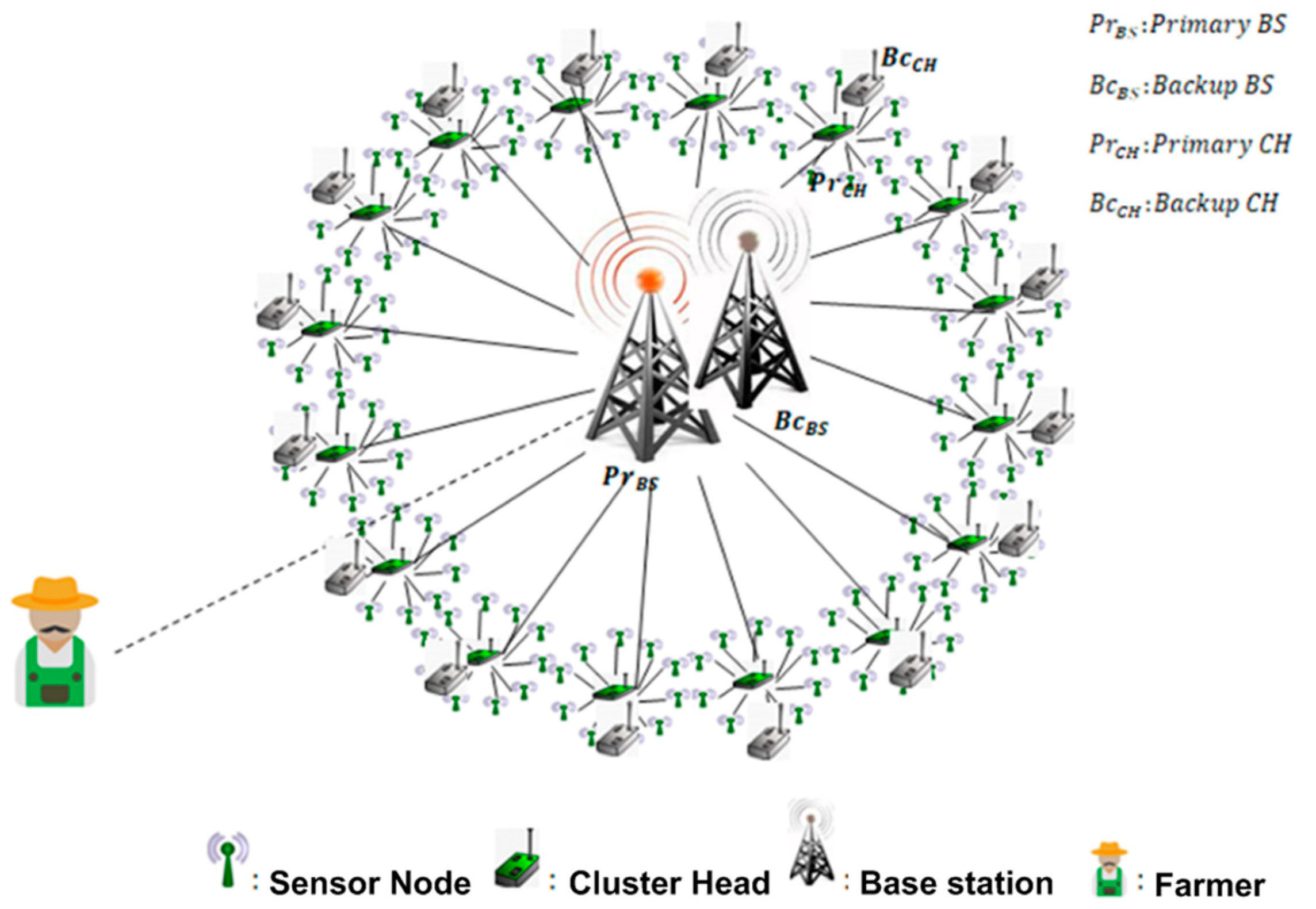
So, our aim here was to construct a safe and a live WSN. In this paper, we propose using the Heartbeat strategy [44,45,46] as a monitoring strategy for failure detection and hardware replication for recovery. The replication refers to the BS and CHs. In anticipation of a possible failure of the primary BS, we have two BSs instead of one: a primary BS and a backup one. Figure 4 shows this scenario. The same would apply to the CHs, i.e., each CH will have a backup CH which will take the role in the case of a failure of the primary CH. By using the mentioned strategies, the fault detection can be provided immediately at the moment of a device crash/failure (i.e., for a CH or BS) and then the faulty device can be replaced immediately with the undamaged backup device.

After having discussed the topology used for the deployment of a WSN in precision agriculture, a fault-tolerant model will be detailed in the following sections. We will use the Uppaal-4.1.26 model checker for the system simulation and property verification.

5.1. Fault-Tolerant Clusters

5.1.1. Sensor Nodes

As we know, the main task of a sensor node is the collection of data from the agricultural field; then, the information is to be transmitted to the primary CH. We already have mentioned before that the sensor nodes enter the passive state just after collecting and sending data in order to minimize the energy consumption. Now, the role of detection of failed sensor nodes is assigned to the leader CH. When the time slot associated with a specific sensor node ID arrives, a data request will be sent from the cluster leader to the sensor node. This sensor then must reply to that request before the timeout. If the timeout occurs without any response, the sensor node will be considered as failed and its ID will be stored in a queue of failed sensor nodes. The list of failed sensor nodes will be sent to the BS by the CH along with the collected data.

5.1.2. Fault-Tolerant CH

Two CHs must be placed (see Figure 4) for our model. The first one has the role of the primary CH, while the other plays the role of the secondary CH. Figure 5 illustrates this concept.

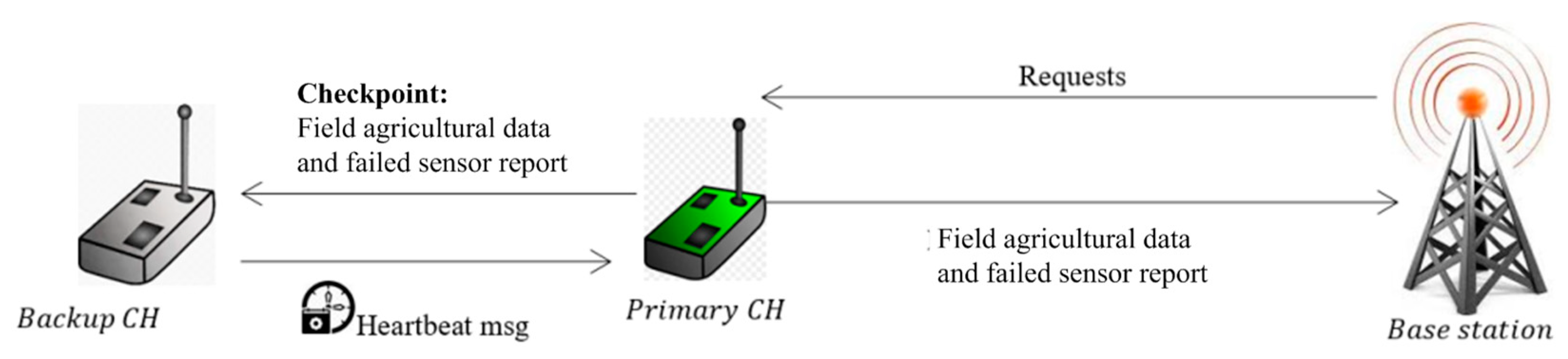
First, an initialization phase has to be performed between the two CHs by communicating the primary CH ID and sensor nodes’ TDMA schedule. This step can be considered as a task assignment in order to start working (initialization). After that, the primary CH takes the role of receiving, aggregating, and transmitting environmental data from the sensor nodes to the BS. In addition, it is responsible for detecting any crashed or failed sensor(s) and providing a report on them to the BS. Furthermore, it keeps the backup CH updated with any data it has received. In this context, it is essential to mention that the primary CH and its backup work in mutual exclusion and each one has its own ID (i.e., identity). It is also possible to use more than one backup CH; it can be two or more and as the number increases, the efficiency also increases for precision agriculture (see Figure 6).

On the other hand, the backup CH is constantly on standby to take over the tasks in the case of a malfunction or breakdown of the primary CH (see Figure 7). Moreover, it is responsible for monitoring the primary CH at all times, and if no Heartbeat message is received, the backup CH will directly assume the tasks and role reversal will take place.

Role reversal: In the case of primary CH failure, the backup CH would broadcast its identity over the cluster and subsequently, it would send a notification carrying the identity of the failed CH to the BS with the aim of promptly repairing it. After that, the new primary CH would start working normally while the previous primary CH would assume the role of the backup CH.

All the steps described above are summarized in Algorithm 3. Instructions 1–24 pertain to the primary CH, while instructions 25–31 are related to the backup CH. The role reversal instructions are cited in lines 32–36. Finally, the sensor node process is presented in instructions 37–43.

Algorithm 3. Fault-tolerant protocol in the cluster

Input: Wireless sensor network

Output: Fault-tolerant cluster communication protocol

1. Primary Cluster Head () 2. initiate clock x: =0; 3. For loop = 1 to n nodes 4.    If $x={time slot}_{loop}$ then 5.       Send Data Request to the ${node}_{loop}$ 6.          If the Primary CH Receives data from ${Node}_{loop}$ then 7.            save $\left({NodeData}_i\right)$ in Sensor_data_file; 8.          Else 9.           If x >= $Node\_TimeOut$ and no data received from the sensor node then 10.              Threads ${node}_{loop}$ in Failed_Sensornodes_File; 11.           End If 12.          End If 12.    End If 14. End For 15.      Aggregate collected data; 16.   If data_request received from the BS then 17.       Send Aggregated Data to the BS; 18.       Send the Failed_Nodes_File to the BS; 19.     End If 20.     If x = Heartbeat_Time then 21.       Send ‘I am alive’ message to the Backup CH; 22.       Send a checkpoint with Aggregated Data and Failed_Sensornodes_File to the Backup CH; 23.     End If 24. End Primary Cluster Head process()

25. Backup Cluster Head() 26.   Initiate clock x: =0; 27.   If x >= Heartbeat_TimeOut and no alive message received from the Primary CH then 28.     Alerte: ‘Failed Pimary CH’ 29.     proceed a roles exchange between the failed Primary CH and the Backup CH; 30. End If 31. End Backup Cluster Head()

32. CH Roles Exchange() 33. Exchange (Primary CH; Backup CH); 34. Broadcast the new Primary CH ID over the cluster; 35. Send a failure alert to the BS with the failed CH ID; 36. End CH Roles Exchange()

37. Sensor node() 38.   If receive data request from the Primary CH then 39.     Go to active state; 40.     Send environment data to the Primary CH; 41.     Go to passive state; 42.   End If 43. End Sensor node()

5.2. Fault-Tolerant Base Station

As our considered scenario is precision agriculture, it is imperative to ensure the correct operation of the BS in order to ensure the accurate transmission of information related to the agricultural field. In fact, any malfunction of the BS can lead to a breakdown of the network and the loss of the collected information. In order to avoid such problems, we used a physical replication approach and this was implemented by using two BSs: a primary BS and a backup BS. Both of these BSs are completely identical in terms of hardware as well as software resources, in addition to their close proximity in the agricultural field to ensure the same distance to the rest of the clusters.

The main function of the primary BS is to execute all the assigned tasks of a Base Station in a WSN. First, it receives the final user’s requests. Then, it sends data requests to the set of CHs. After that, it receives the collected information as well as the list of failed equipment (i.e., failed sensor nodes and failed CHs). Finally, it sends the collected data to the final user. On the other hand, the role of the backup BS is solely to monitor the primary BS and store an updated version of the collected data as well as the most recent request received from the final user. Figure 8 illustrates this concept.

In the event of a failure or malfunction of the primary BS, the backup BS takes over the tasks seamlessly, and the WSN continues to function normally without any interruption as if no failure occurred. This is based on the assumption that the backup BS possesses all the necessary data to fulfil the tasks. In this context, it is essential to mention again that the activation of the primary BS and its backup is mutually exclusive and each one has its own ID (i.e., identification number). To start operating, an initialization step must be carried out between the primary BS and its backup by preparing themselves to work in rotation (when need be) and this can be achieved by exchanging the necessary information before starting the task. The primary information includes the primary BS ID and the set of CHs’ TDMA schedule.

After that, the primary BS takes on the tasks of collecting the data received from the CHs in addition to the specific data concerning sensor node and CH failures. The primary BS then reduces the amount of information by aggregating the data into a single packet, which is sent to the final user (see Figure 9). One of the additional tasks for the primary BS is to keep the backup station informed about all WSN updates and development through regular updates (i.e., checkpoints).

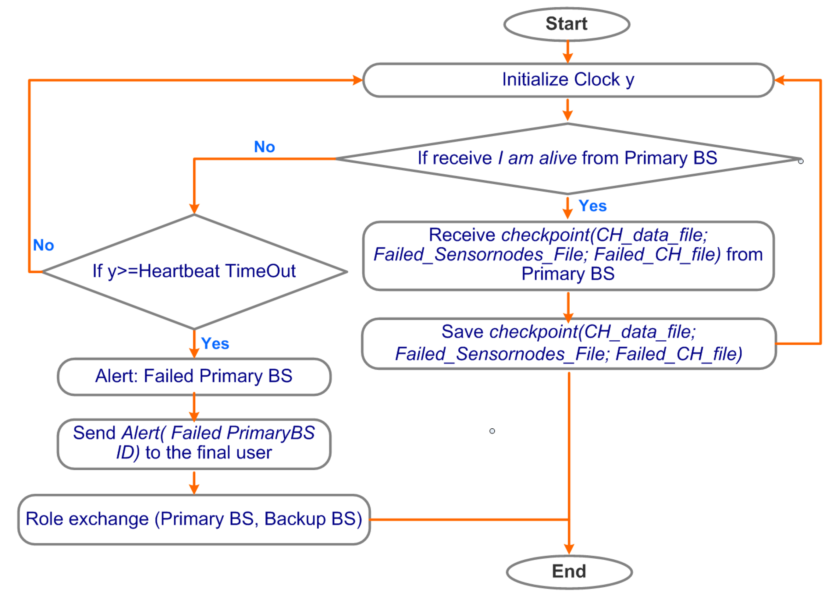
Again, the backup BS is ready to take over at any moment after the detection of a primary BS failure. The fault detection is provided when the live message is not received from the primary BS within the allocated Heartbeat time. In that event, the primary BS is considered as faulty and the role reversal is implemented immediately (see Figure 10).

Hence, in the case of a fault detection, the Primary BS is replaced immediately by the Backup BS. The new Primary BS then sends a failure alert to the final user containing the failed Primary BS identity, for the purpose of repairing. The new Primary BS also broadcasts its identity over the WSN and then assumes the Primary BS’s tasks. After fixing the issue, it takes over the role of the Backup BS. It should be reiterated here that it is also possible to use more than one Backup BSs. In fact, the Backup BS acts as an emergency redundant device for the Primary station in the event of its failure or shutdown. Such redundancy ensures the continuity and operation of the system even if any issue arises with the Primary BS (for which it is incapable of functioning properly). Therefore, the Backup BS possesses all the necessary information and resources to perform the tasks assigned to the Primary BS to carry on with the operation whenever required. This contributes to achieving self-stability and efficiency of the system over time. These processes are summarized in Algorithm 4.

Algorithm 4. Fault-tolerant Base Station protocol

Input: Base Station process

Output: Fault-tolerant Base Station

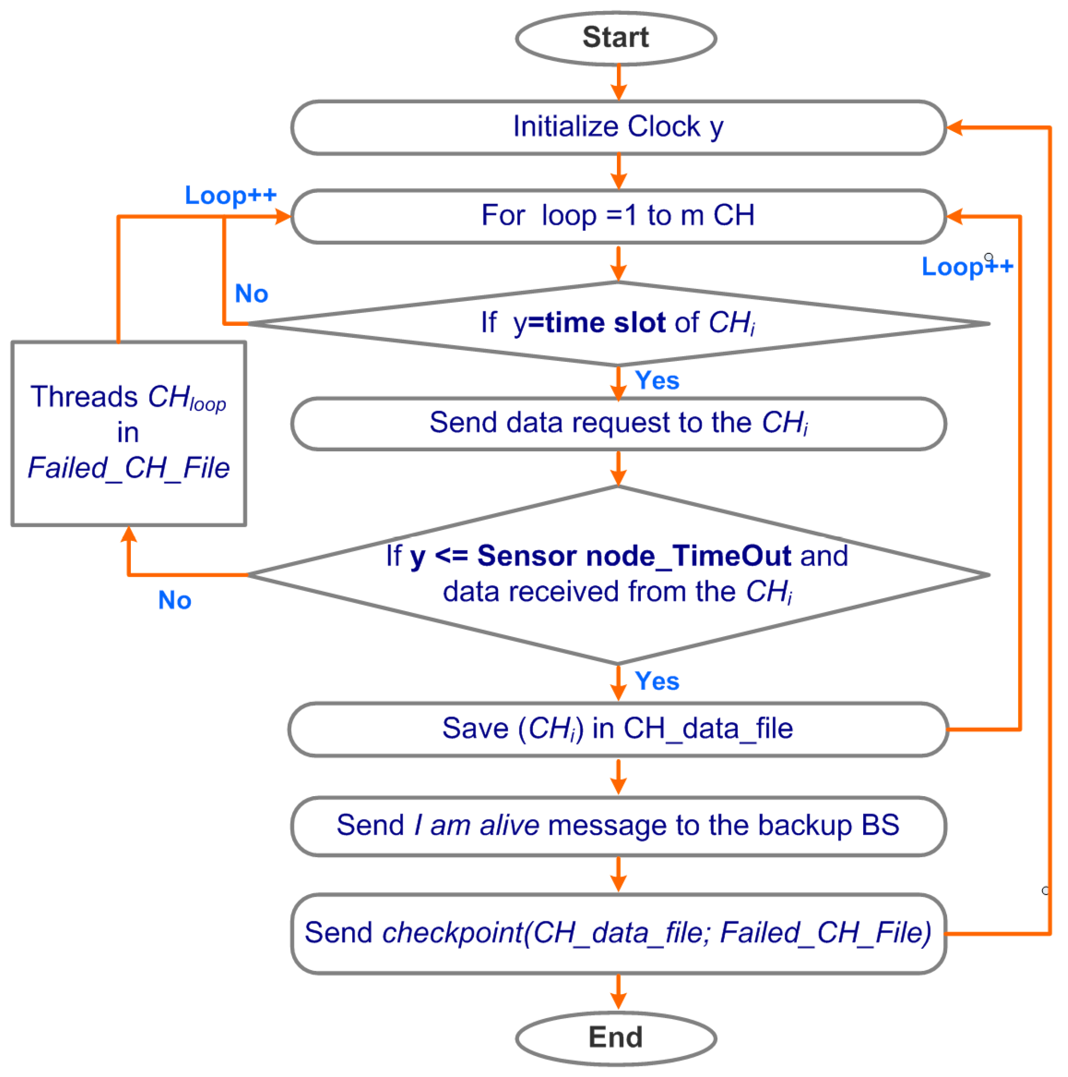
1.     Primary Base station() 2.     Initialize clock y = 0 3.     For loop = 1 to m CH 4.       If y = ${time slot}_{loop}$ then 5.         Send data request to the Primary CH; 6.         Receive aggregated data from the Primary CH; 7.         save CH data in CH_Data_File; 8.       End If 9.       If y >= CH_TimeOut and data not received from CH then 10.         Threads CH ID in Failed_CH_file; 11.       End If 12.     End For 13. Send CH_Data_File and Failed_CH_file to the End user; 14. Send Checkpoint (DataFile, Failed_CH_file)to the Backup BS; 15. If y = BS_Heartbeat_time then 16.       Send “I am alive” to the Backup BS 17. End If 18. End Primary Base station()

19. Backup Base station() 20. Initiate clock y; 21.   If y >= BS_Heartbeat_TimeOut and the no alive message received from the Primary BS then 22.     Alerte: ‘Failed Primary BS’; 23.    proceed the roles exchange between the failed Primary BS and the Backup BS; 24.   End If 25. End Backup Base station()

26. BS Roles Exchange() 27.   Exchange (Primary BS; Backup BS); 28.   Broadcast the new Primary BS ID over the cluster; 29.   Send a failure alert to the end user with the failed BS ID; 30. End BS Roles Exchange()

6. Formal Verification of the Fault-Tolerant Model

In this section, we present our simulation and a formal verification using the UPPAAL model checker for our fault-tolerant WSN model intended for the agricultural field. The Uppaal-4.1.26 framework is considered a sophisticated tool for verifying timed system models [47]. The framework is based on the theory of timed automata but it has been extended to support features required by the real-time system and protocol verification community. The query language of UPPAAL that is used to specify properties (that are to be checked) is a subset of TCTL (Timed Computation Tree Logic). TCTL is a formal temporal logic used for specifying and verifying temporal properties in timed systems. In fact, the UPPAAL model checker can provide a formal verification of the safety and liveness properties.

For the readers, it may be mentioned again here that the safety property ensures that some undesirables scenarios are not reachable while the liveness property guarantees that certain desirable states are eventually achieved. UPPAAL’s model checking capabilities use formal methods to systematically explore the system state space and validate whether the system satisfies these safety and liveness requirements in order to ensure the correctness and fault tolerance of the WSN system.

6.1. Formal Model

As shown in Figure 11, a set of timed automata were designed for each WSN component: (a) PrimaryCH (i.e., primary Cluster Head), (b) BackupCH (i.e., backup Cluster Head), (c) EndUser (i.e., the end user), (d) PrimaryBS (i.e., primary Base Station), (e) BackupBS (i.e., backup Base Station), (f) SensorNode (i.e., sensor node).

6.2. Simulation

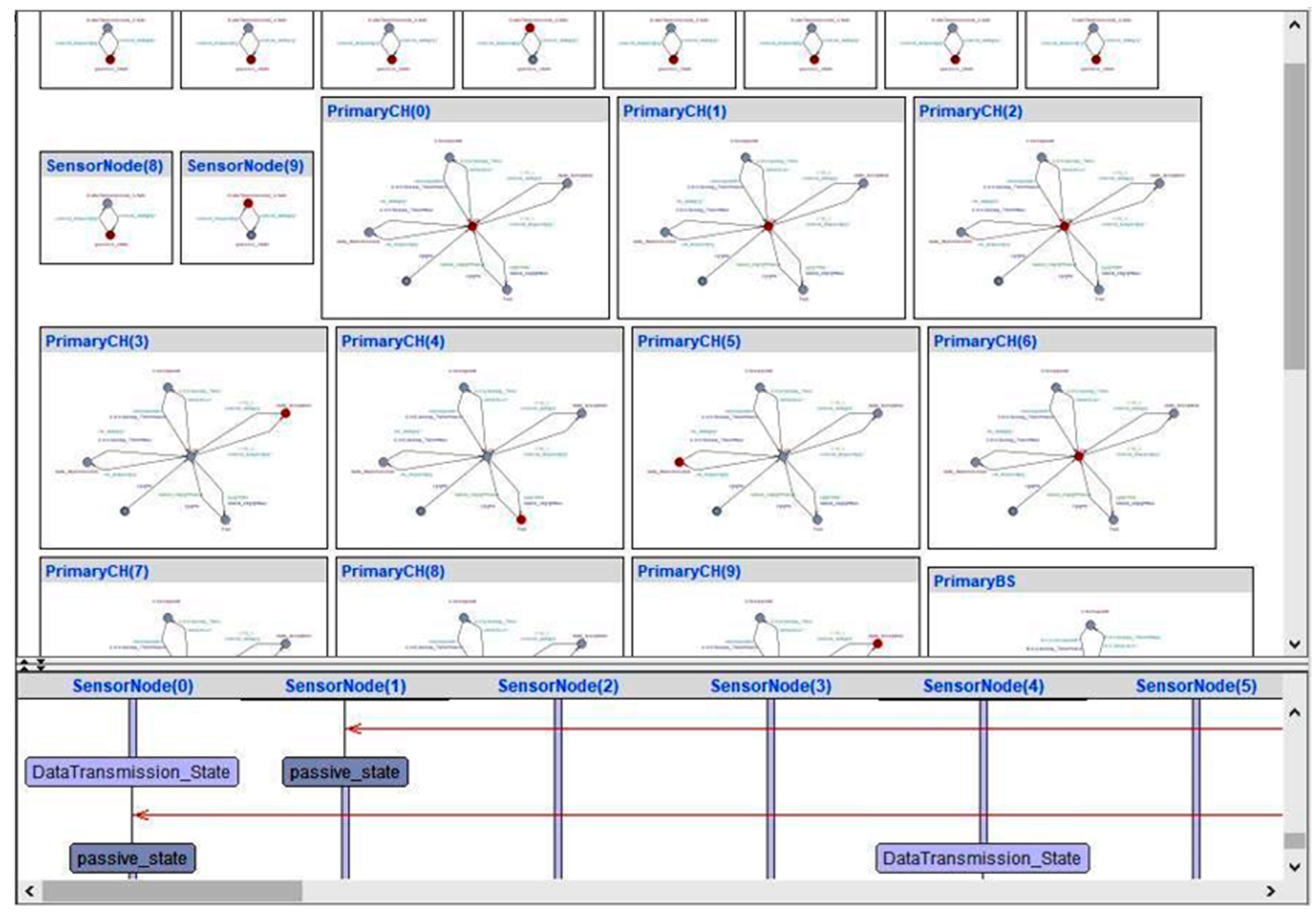
After designing the set of fault-tolerant WSN components using real-time timed automata and programming the necessary variables, clocks, and synchronization channels, the model simulation was obtained, as shown in Figure 12.

Here, the WSN was composed of 1 primary BS, 1 backup BS, and 10 clusters. Each cluster is composed of 1 primary CH, 1 backup CH, and 10 sensor nodes. To enable observation of the fault tolerance behavior of the model (i.e., the backup component behavior), two clocks were used to schedule the failure of both BSs (i.e., the primary BS and backup BS) and CHs (i.e., the primary CH and backup CH).

6.3. Verification of the Properties

In this part of the formal verification, a set of safety and liveness properties of the fault-tolerant WSN’s formal model were tested. The set of properties are summarized in

Table 1. Safety and liveness properties.

Type	TCTL queries	Description
Safety	A[] not deadlock	The WSN never reaches a deadlock state.
	A<> forall (i:id_c) not(PrimaryCH(i).Fail and BackupCH(i).Fail)	The primary CH and the backup CH never fail at the same time.
	A<> forall (i:id_c) not (PrimaryCH(i). Safe and BackupCH(i).Safe)	The primary CH and its backup are in mutual exclusion.
	A<>not(PrimaryBS.Failed and BackupBS.Failed)	The primary BS and the backup BS never fail at the same time.
	A<>(PrimaryBS.Safe imply BackupBS.Fail) and (PrimaryBS.Fail imply BackupBS.Safe)	The primary BS and its backup are operating in mutual exclusion.
Liveness	A<>forall (i:id_s) forall (j:id_c) (SensorNode(i). DataTransmission_State imply (PrimaryCH(j).data_reception or BackupCH(j).data_reception))	The collected data sent by the sensor node are always received by the primary CH or the backup CH.
	A<> forall(i: id_c) (PrimaryCH(i). data_transmission or BackupCH(i).data_transmission) imply (PrimaryBS.data_reception or BackupBS.data_reception)	The aggregated data sent by the CH are always received by the primary or the backup BS.
	E<> EndUser.Data_reception	The WSN always offers data for the end user.
	A<> forall (i:id_c) (z[i] >= 50 imply (PrimaryCH(i).Fail and BackupCH(i).Safe))	After energy depletion of the primary CH, the backup CH takes over the role.
	A<> zz >= 100 imply PrimaryBS.Fail and BackupBS.Safe	The backup BS completes the task after the energy depletion of the primary BS.
	A<> forall (i:id_c) (PrimaryCH(i).Fail imply BackupCH(i).Safe) and (BackupCH(i). Fail imply PrimaryCH(i).Safe)	There is always one CH in operation (i.e., the primary or backup CH)
	A<> (PrimaryBS.Fail imply BackupBS.Safe) and (BackupBS.Fail imply PrimaryBS.Safe)	There is always one BS in service.

. TCTL formal temporal logic was used to specify the temporal properties.

The property verification results are shown in Figure 13. As shown in the figure, it is evident that all the requirements are satisfied by the model, indicating the effectiveness of the proposed fault-tolerant scheme in both failure detection and correction.

7. Complexity Estimation of the Fault-Tolerant WSN Model

After confirming the effectiveness of the proposed model by using UPPAAL formal verification, it is essential to estimate its complexity.

7.1. Estimation of Message Density

Let us assume that the function $f(\alpha ,\beta )$ refers to the transmitted messages in the WSN. Then, $f\left(\alpha ,\beta \right)=1+2\alpha \left(1+\beta \right)$ (i.e., CH, sensor node) represents the transferred messages between the different components in the WSN. The set of transferred messages is resumed in requests and data transactions. Let us assume a second function, $g(\alpha ,\beta ,\gamma )$, which refers to the transmitted messages in a fault-tolerant WSN. Therefore, $g\left(\alpha ,\beta ,\gamma \right)=1+2\alpha \left(1+\beta \right)+2\gamma \left(1+\alpha \right)$ (i.e., $\gamma$: the Backup’s component number). In such a case, the different types of transmitted messages can be requests, data, checkpoint, and alive messages.

As we can see in Figure 14 and Figure 15, it is evident that the densities of exchanged messages were similar between the regular WSN and the fault-tolerant WSN. In fact, the fault-tolerant WSN had two additional types of messages: the first one is related to checkpoints whereas the second type concerns the Heartbeat message. Despite that, we can observe that it did not have any significant impact on the message density of the network (see Figure 15). It is clear that the highest percentage was for request and data messages while the lowest percentage was for the checkpoint and Heartbeat messages.

Based on what has been mentioned before, we can conclude that the proposed scheme does not have a major effect on the load of the communication link due to synchronization messages. Subsequently, we attempted to estimate the response time.

7.2. Estimation of Response Time

In this section, we attempt to estimate the delay required to send data to the final user (i.e., the farmer). For this, the fault-tolerant WSN model was simulated in various situations with a constant number of sensor nodes (i.e., 10 sensor nodes) and a different number of CHs in order to increase the WSN scalability. The primary CH is supposed to exhaust its energy at time 50; after that, the backup CH takes over the role.

The BS energy depletion time is supposed to be at 100 units of time; after that, the backup BS starts operating. Both the backup CH and backup BS operate for 80 units of time and after that, the repaired primary component (i.e., CH, BS) takes over (see

Table 2. Energy depletion of fault-tolerant WSN component.

Component	Energy Depletion (Joules)
Primary CH	50
Primary BS	100
Backup CH	80
Backup BS	80

). In order to simulate the component energy depletion, we used variables in decremented loops.

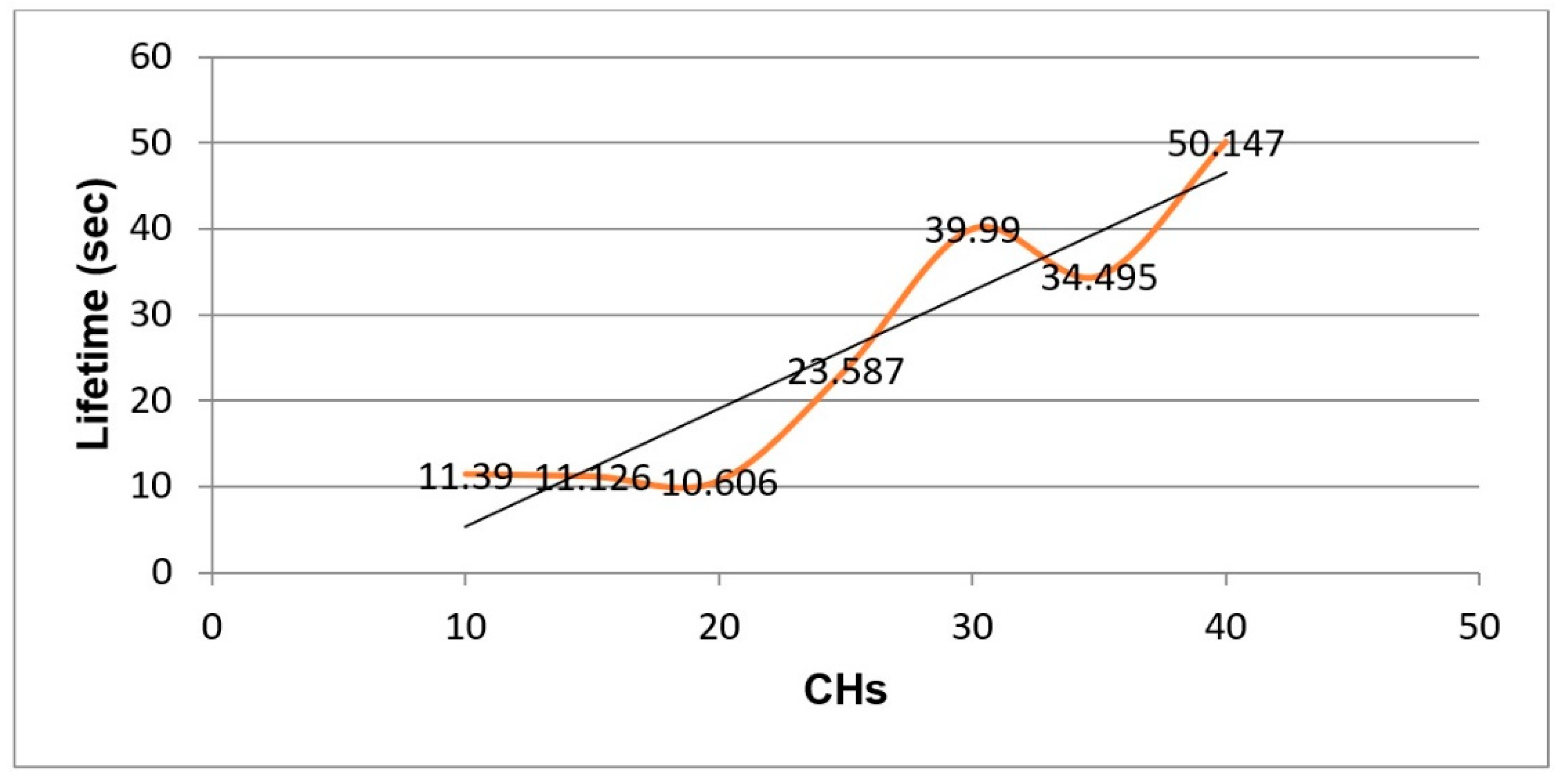
In each simulation cycle, the delay required for the end user to receive data was recorded; the collected data are summarized as plots in Figure 16. On the other hand, a regular WSN (i.e., a non-fault-tolerant WSN) was simulated with the same conditions. For this case, the WSN’s lifetime measures are presented in Figure 17.

In Figure 16, we can see that the response time did not have a consistent pattern; we can observe that in the case of 20 CHs, the response time delay was larger than that of 30 CHs. It should be noted here that the scenario of fault detection and role reversal between failed and healthy components result in this delay and we can say that the system goes through a non-stabilization state before the backup components take over the role and this requires some time that will certainly impact the overall response time. Considering this point, a well-designed WSN, with a well-studied number of components, can minimize this effect. We can also observe that the response time increased with the scale of the WSN; in fact, this situation is common for all WSNs. Generally, we can say that the response time delays are reasonable and the use of the fault tolerance strategy does not lead to any drastic decrease in the WSN’s service quality.

In Figure 17, we can observe that the non-fault-tolerant WSN’s lifetime was very short (i.e., between 10 and 50). Furthermore, sometimes the WSN stopped operating before sending data to the final user. Hence, the availability of the WSN was not guaranteed. This can cause irreparable damage in the agricultural field due to the data loss.

Regarding Figure 16 and Figure 17, it can be noticed that even though the response time was sometimes long in the case of the fault-tolerant WSN, the availability was still guaranteed. Hence, the WSN continued to provide the final user with the indispensable data without any interruptions. This last feature is very important in such systems.

Based on all of the above, we can conclude that the proposed scheme for fault tolerance in WSNs provides a safe and available service.

7.3. Comparative Analysis

Table 3. Feature comparison.

Reference	Fault detection Mechanism	Fault Tolerance Mechanism	Fault type	Advantage	Limitations
[35]	Particle swarm optimization for faulty node detection	Selection of the CH on the basis of residual energy, coverage, etc. Fault-free paths determined using Genetic Algorithm and self-healing method was employed to resolve network connectivity issues.	Energy depletion, connection failure	Lower energy consumption and lower packet loss ratio	Congestion, extended delays, and protocol complexity
[39]	None	Backup CH selection using fuzzy logic technique.	Cluster member energy depletion and hardware errors	Fast fault detection and recovery	Network energy depletion and congestion
[40]	None	Topology construction method based on potential game and cut vertex detection.	Network energy depletion	Reduction in energy consumption and increased energy efficiency	Extended delays, cluster construction protocol complexity, and congestion
[48]	None	System reliability prediction and Fault Tree Analysis.	Hardware failures and communication errors	Design and implementation of a reliable WSN by considering environmental conditions	Used only for small-scale WSN; difficult to predict possible failures
[49]	None	CH selection by using the battle royal optimization algorithm; data communication enhancement by selecting a backup CH; and the aggregator node is selected using the Particle Swarm Optimization method.	Battery drain, network failure, node breakdown	Reliable network, increased energy efficiency	Extended delays and protocol heaviness; congestion
Our Proposal	CH and BS fault detection using the Heartbeat strategy	CH and BS hardware redundancy and forward recovery.	Energy depletion and hardware faults of sensor nodes, CH, and BS	Quick fault detection and recovery, prolonged WSN lifetime, offers continuous service	Cost due to hardware redundancy; only convenient for small-scale WSNs

presents a comparative analysis between some recent works and our proposed scheme. Obviously, the main objective of the vast majority of research works was to reduce the energy consumption and to extend the WSN’s lifetime. However, it is evident that fault detection has not been extensively addressed by the majority of the proposed solutions. Furthermore, the most effective methods result in a lot of complexities. This inevitably leads to significant delays and congested connections. In our proposal, we address energy depletion and hardware errors for fault tolerance through the sensor nodes, Cluster Heads, and Base Station without adding much complexity and without affecting the response delays or network load. In fact, the fault detection strategy has received its due attention as an integral part of the fault tolerance technique.

7.4. Discussion on the Other Cost Issues

One of the issues that define the practicality of a WSN application is its deployment cost [50]. In our setting, we consider precision agriculture where the user can physically reach various locations on the crop field. Hence, unlike other regular WSN settings, this is not an inaccessible terrain and the user is able to deploy, fix, and even replace devices at specific locations. Hence, the cost associated with deployment via other means (aircraft, drones, etc.) is not applicable in our case. In fact, when planting the crops or seeds, the farmer needs to walk around and go to different parts of the field where the necessary tasks for the deployment of the WSN can also be performed.

Again, if the monetary cost associated with redundant devices is considered, we would argue that the protection offered by such a WSN from the potential loss or damage of crops (due to perhaps, random weather events, lack of proper irrigation, and so on) is much greater than the monetary cost for deploying those extra devices. The functions are also pretty simple and easy to maintain. The fault-tolerant scheme makes sure the WSN does not fail even in the case of failure of key primary components. If the faulty or failed device is physically taken away after a failure event takes place, it is possible to repair it so that it can be used again in such a setting. Hence, this is feasible and cost-effective solution for precision agriculture scenarios.

8. Conclusions and Future Work

In this paper, we considered a precision agriculture setting where a WSN is used with a specific deployment pattern. We proposed a fault-tolerant scheme for energy efficiency based on hardware redundancy. The key idea is based on using hardware redundancy at the level of the Cluster Heads and Base Station, by using a primary and one or more backup devices. At each level, the primary device and its backup will exchange roles in the event of a failure. In this way, the continuity of the WSN (deployed for the crop field) in providing essential services (despite the occurrence of faults) can be ensured.

To ensure the effectiveness of this approach, it is essential to provide the backup device (i.e., CH and Base Station) with all the necessary checkpoints about the WSN so that it is fully ready to take over the tasks. It is worth noting that the fault detection is achieved using Heartbeat strategies, where the primary CH plays the role of the sensor nodes’ fault detector when it monitors the set of CHs. Meanwhile, the backup device monitors the primary one. Sleep mode technology is used at the sensor node level to conserve energy and extend the battery life. In order to validate the effectiveness of the proposed scheme, a system simulation was provided using the UPPAAL model checker tool for real-time systems. The fault tolerance properties (i.e., safety and liveness) of the model were rigorously tested, and the results demonstrate the efficacy of the proposed scheme in fault detection and continuous service delivery. A comparative chart with some previous works was provided in order to show the effectiveness of the proposed model.

As a future work based on this work, we aim to implement this scheme in real-life settings of WSNs in order to highlight its strengths and limitations and to compare it with the other existing strategies. Moreover, we aim to enhance the scheme to address the issues of scalability and applicability with diverse types of network architectures.

References

- Kashyap, R. Applications of Wireless Sensor Networks in Healthcare. In IoT and WSN Applications for Modern Agricultural Advancements: Emerging Research and Opportunities; IGI Global: Hershey, PA, USA, 2020; pp. 8–40. [Google Scholar] [CrossRef]
- Morrow, M.; MaWhinney, S.; Brooks, K.M.; Huntley, R.; Castillo-Mancilla, J.R.; Anderson, P.L.; Kiser, J.J. Improving the accuracy of adherence data collected using medication monitoring technology in clinical research. Contemp. Clin. Trials 2023, 125, 107051. [Google Scholar] [CrossRef]
- Honda, S.; Hara, H.; Arie, T.; Akita, S. A wearable, flexible sensor for real-time, home monitoring of sleep apnea. iScience 2022, 25, 104163. [Google Scholar] [CrossRef] [PubMed]
- Jurak, J.; Osman, K.; Sikirić, M.; Šimunović, L. Wireless Sensor Network Architecture for Passenger Counting in Public Transportation. Transp. Res. Procedia 2023, 73, 227–232. [Google Scholar] [CrossRef]
- Srividya, K.S.; Hemavathi, S.; Roselyn, P. Design of an efficient energy management system for renewables based wireless electric vehicle charging station. Energy Storage 2023, 5, e454. [Google Scholar] [CrossRef]
- Akilan, T.; Baalamurugan, K.M. Automated weather forecasting and field monitoring using GRU-CNN model along with IoT to support precision agriculture. Expert Syst. Appl. 2024, 249, 123468. [Google Scholar] [CrossRef]
- Kho, E.P.; Chua, S.N.D.; Lim, S.F.; Lau, L.C.; Gani, M.T.N. Development of young sago palm environmental monitoring system with wireless sensor networks. Comput. Electron. Agric. 2022, 193, 106723. [Google Scholar] [CrossRef]
- Si, L.F.; Li, M.; He, L. Farmland monitoring and livestock management based on internet of things. Internet Things 2022, 19, 100581. [Google Scholar] [CrossRef]
- Sohraby, K.; Minoli, D.; Znati, T. Wireless Sensor Networks: Technology, Protocols, and Applications; Wiley: Hoboken, NJ, USA, 2007; ISBN 978-0-470-11275-5. [Google Scholar]
- Akyildiz, I.F.; Su, W.; Sankarasubramaniam, Y.; Cayirci, E. Wireless sensor networks: A survey. Comput. Netw. 2002, 38, 393–422. [Google Scholar] [CrossRef]
- Casares-Giner, V.; Navas, T.I.; Flórez, D.S.; Hernández, T.R.V. End to End Delay and Energy Consumption in a Two Tier Cluster Hierarchical Wireless Sensor Networks. Information 2019, 10, 135. [Google Scholar] [CrossRef]
- Fischione, C. An Introduction to Wireless Sensor Networks. Royal Institute of Technology: Stockholm Version1. , September 2014. Available online: https://www.kth.se/social/files/5431a388f276540a05ad2514/An_Introduction_WSNS_V1.8.pdf (accessed on 21 March 2024).
- Marwa, C.; Othman, S.B.; Sakli, H. IoT based low-cost weather station and monitoring system for smart agriculture. In Proceedings of the 2020 20th International Conference on Sciences and Techniques of Automatic Control and Computer Engineering (STA), Monastir, Tunisia, 20–22 December 2020; pp. 349–354. [Google Scholar]
- Hewage, P.; Behera, A.; Trovati, M.; Pereira, E.; Ghahremani, M.; Palmieri, F.; Liu, Y. Temporal convolutional neural (TCN) network for an effective weather forecasting using time-series data from the local weather station. Soft Comput. 2020, 24, 16453–16482. [Google Scholar] [CrossRef]
- Ramdoo, V.D.; Khedo, K.K.; Bhoyroo, V. A flexible and reliable wireless sensor network architecture for precision agriculture in a tomato greenhouse. In Information Systems Design and Intelligent Applications; Advances in Intelligent Systems and Computing (AISC); Satapathy, S., Bhateja, V., Somanah, R., Yang, X.S., Senkerik, R., Eds.; Springer: Singapore, 2019; Volume 863. [Google Scholar]
- Martinho, V.J.P.D.; Guine, R.d.P.F. Integrated-smart agriculture: Contexts and assumptions for a broader concept. Agronomy 2021, 11, 1568. [Google Scholar] [CrossRef]
- Dholu, M.; Ghodinde, K.A. Internet of Things (IoT) for Precision Agriculture Application. In Proceedings of the 2018 2nd International Conference on Trends in Electronics and Informatics (ICOEI), Tirunelveli, India, 11–12 May 2018; pp. 339–342. [Google Scholar]
- Matin, M.A.; Islam, M.M. Overview of Wireless Sensor Network. In Wireless Sensor Networks—Technology and Protocols; Matin, M.A., Ed.; IntechOpen: London, UK, 2012. [Google Scholar] [CrossRef]
- Yick, J.; Mukherjee, B.; Ghosal, D. Wireless sensor network survey. Comput. Netw. 2008, 52, 2292–2330. [Google Scholar] [CrossRef]
- Chouikhi, S.; El Korbi, I.; Ghamri-Doudane, Y.; Saidane, L.A. A survey on fault tolerance in small and large scale wireless sensor networks. Comput. Commun. 2015, 69, 22–37. [Google Scholar] [CrossRef]
- Flores, K.O.; Butaslac, I.M.; Gonzales, J.E.M.; Dumlao, S.M.G.; Reyes, R.S. Precision agriculture monitoring system using wireless sensor network and Raspberry Pi local server. In Proceedings of the 2016 IEEE Region 10 Conference (TENCON), Singapore, 22–25 November 2016. [Google Scholar]
- Hamouda, Y.E.; Elhabil, B.H. Precision Agriculture for Greenhouses Using a Wireless Sensor Network. In Proceedings of the 2017 Palestinian International Conference on Information and Communication Technology (PICICT), Gaza, Palestine, 8–9 May 2017. [Google Scholar]
- Mat, I.; Kassim, M.R.M.; Harun, A.N. Precision agriculture applications using wireless moisture sensor network. In Proceedings of the 2015 IEEE 12th Malaysia International Conference on Communications (MICC), Kuching, Malaysia, 23–25 November 2015. [Google Scholar]
- Sarkar, I.; Pal, B.; Datta, A.; Roy, S. Wi-Fi-based portable weather station for monitoring temperature, relative humidity, pressure, precipitation, wind speed, and direction. In Information and Communication Technology for Sustainable Development; Advances in Intelligent Systems and Computing book series (AISC); Tuba, M., Akashe, S., Joshi, A., Eds.; Springer: Berlin/Heidelberg, Germany, 2020; Volume 933, pp. 399–404. [Google Scholar]
- Zhang, J.; Guan, K.; Peng, B.; Jiang, C.; Zhou, W.; Yang, Y.; Pan, M.; Franz, T.E.; Heeren, D.M.; Rudnick, D.R.; et al. Challenges and opportunities in precision irrigation decision-support systems for center pivots. Environ. Res. Lett. 2021, 16, 053003. [Google Scholar] [CrossRef]
- Singh, D.K.; Sobti, R. Development of Wi-Fi-Based Weather Station WSN-Node for Precision Irrigation in Agriculture 4.0. In Emergent Converging Technologies and Biomedical Systems; Lecture Notes in Electrical Engineering Book Series (LNEE); Marriwala, N., Tripathi, C.C., Jain, S., Mathapathi, S., Eds.; Springer: Berlin/Heidelberg, Germany, 2022; Volume 841. [Google Scholar]
- Ojha, T.; Misra, S.; Raghuwanshi, N.S. Wireless sensor networks for agriculture: The state-of-the-art in practice and future challenges. Comput. Electron. Agric. 2015, 118, 66–84. [Google Scholar] [CrossRef]
- Mohapatra, H.; Rath, A.K. Fault tolerance through energy balanced cluster formation (EBCF) in WSN. In Smart Innovations in Communication and Computational Sciences; Advances in Intelligent Systems and Computing (AISC); Tiwari, S., Trivedi, M., Mishra, K., Misra, A., Kumar, K., Eds.; Springer: Berlin/Heidelberg, Germany, 2019; Volume 851. [Google Scholar]
- Kanouni, L.; Semchedine, F. A new paradigm for multi-path routing protocol for data delivery in wireless sensor networks. Int. J. Comput. Appl. 2022, 44, 939–952. [Google Scholar] [CrossRef]
- Pathan, A.-S.K.; Lee, H.-W.; Hong, C.S. Security in Wireless Sensor Networks: Issues and Challenges. In Proceedings of the 8th International Conference on Advanced Communication Technology (IEEE ICACT 2006), Volume II, Phoenix Park, Republic of Korea, 20–22 February 2006; pp. 1043–1048. [Google Scholar]
- Shyama, M.; Pillai, A.S. Fault-tolerant techniques for wireless sensor network—A comprehensive survey. In Innovations in Electronics and Communication Engineering; Lecture Notes in Networks and Systems (LNNS); Saini, H., Singh, R., Kumar, G., Rather, G., Santhi, K., Eds.; Springer: Berlin/Heidelberg, Germany, 2019; Volume 65. [Google Scholar]
- Sheth, H.; Jani, R. Fault tolerance and detection in wireless sensor networks. In Data Science and Intelligent Applications; Lecture Notes on Data Engineering and Communications Technologies (LNDECT); Kotecha, K., Piuri, V., Shah, H., Patel, R., Eds.; Springer: Berlin/Heidelberg, Germany, 2021; Volume 52. [Google Scholar]
- Shankar, A.; Sivakumar, N.R.; Sivaram, M.; Ambikapathy, A.; Nguyen, T.K.; Dhasarathan, V. Increasing fault tolerance ability and network lifetime with clustered pollination in wireless sensor networks. J. Ambient Intell. Humaniz. Comput. 2021, 12, 2285–2298. [Google Scholar] [CrossRef]
- Al-Hawri, E.; Al-Tam, F.; Correia, N.; Barradas, A. Probabilistic Network Coding for Reliable Wireless Sensor Networks. In Proceedings of the 11th Doctoral Conference on Computing, Electrical and Industrial Systems (DoCEIS), Costa de Caparica, Portugal, 1–3 July 2020; pp. 129–136. [Google Scholar]
- Shyama, M.; Pillai, A.S.; Anpalagan, A. Self-healing and optimal fault tolerant routing in wireless sensor networks using genetical swarm optimization. Comput. Netw. 2022, 217, 109359. [Google Scholar]
- Hallafi, A.; Barati, A.; Barati, H. A distributed energy-efficient coverage holes detection and recovery method in wireless sensor networks using the grasshopper optimization algorithm. J. Ambient. Intell. Humaniz. Comput. 2023, 14, 13697–13711. [Google Scholar] [CrossRef]
- Papi, F.; Barati, H. HDRM: A hole detection and recovery method in wireless sensor network. Int. J. Commun. Syst. 2022, 35, e5120. [Google Scholar] [CrossRef]
- Swain, R.R.; Khilar, P.M.; Dash, T. Fault diagnosis and its prediction in wireless sensor networks using regressional learning to achieve fault tolerance. Int. J. Commun. Syst. 2018, 31, e3769. [Google Scholar] [CrossRef]
- Goyal, N.; Dave, M.; Verma, A.K. A novel fault detection and recovery technique for cluster-based underwater wireless sensor networks. Int. J. Commun. Syst. 2018, 31, e3485. [Google Scholar] [CrossRef]
- Wu, H.; Han, X.; Yang, B.; Miao, Y.; Zhu, H. Fault-Tolerant Topology of Agricultural Wireless Sensor Networks Based on a Double Price Function. Agronomy 2022, 12, 837. [Google Scholar] [CrossRef]
- Mahesh, N.; Vijayachitra, S. DECSA: Hybrid dolphin echolocation and crow search optimization for cluster-based energy-aware routing in WSN. Neural Comput. Appl. 2019, 31, 47–62. [Google Scholar] [CrossRef]
- Wymeersch, H.; Eryilmaz, A. Multiple access control in wireless networks. In Academic Press Library in Mobile and Wireless Communications Transmission Techniques for Digital Communications; Academic Press: Cambridge, MA, USA, 2016; pp. 435–465. [Google Scholar]
- Murugan, K.; Pathan, A.-S.K. Prolonging the Lifetime of Wireless Sensor Networks using Secondary Sink Nodes. Telecommun. Syst. 2016, 62, 347–361. [Google Scholar] [CrossRef]
- Chandra, T.D.; Toueg, S. Unreliable failure detectors for reliable distributed systems. J. ACM 1996, 43, 225–267. [Google Scholar] [CrossRef]
- Bertier, M.; Marin, O.; Sens, P. Implementation and performance evaluation of an adaptable failure detector. In Proceedings of the International Conference on Dependable Systems and Networks, Washington, DC, USA, 23–26 June 2002. [Google Scholar]
- Gupta, I.; Chandra, T.D.; Goldszmidt, G.S. On scalable and efficient distributed failure detectors. In Proceedings of the ACM Symposium on Principles of Distributed Computing (PODC’01), Newport, RI, USA, 26–29 August 2001; pp. 170–179. [Google Scholar]
- Behrmann, G.; David, A.; Larsen, K.G. A Tutorial on Uppaal 4.0. Department of Computer Science, Aalborg University: Denmark, 2006. Available online: https://www.it.uu.se/research/group/darts/papers/texts/new-tutorial.pdf (accessed on 28 August 2023).
- Catelani, M.; Ciani, L.; Bartolini, A.; Del Rio, C.; Guidi, G.; Patrizi, G. Reliability analysis of wireless sensor network for smart farming applications. Sensors 2021, 21, 7683. [Google Scholar] [CrossRef]
- Rani, K.P.; Sreedevi, P.; Poornima, E.; Sri, T.S. FTOR-Mod PSO: A fault tolerance and an optimal relay node selection algorithm for wireless sensor networks using modified PSO. Knowl.-Based Syst. 2023, 272, 110583. [Google Scholar] [CrossRef]
- Pathan, A.-S.K. Security of Self-Organizing Networks: MANET, WSN, WMN, VANET; Auerbach Publications: Boca Raton, FL, USA; CRC Press: Boca Raton, FL, USA; Taylor & Francis Group: Abingdon, UK, 2010; ISBN 978-1-4398-1919-7. [Google Scholar]
Figure 1.
WSN hierarchical topology.
Figure 2.
CH and sensor node routing protocol: (a) cluster construction; (b) data transfer.
Figure 3.
CH and BS communication protocol: (a) initialization; (b) data transfer.
Figure 4.
Fault-tolerant WSN model for precision agriculture.
Figure 5.
Fault-tolerant Cluster Head.
Figure 6.
Fault-tolerant primary CH process.
Figure 7.
Fault-tolerant backup CH process.