1. Introduction
The exponential rise in the usage of the Internet has led to e-commerce rapidly becoming an integral part of modern society. The increasing use of portable devices enables more frequent as well as faster access to the Internet, which makes online shopping and digital marketplaces now a ubiquitous presence in the lives of consumers around the world [
1]. This is also shown by the e-commerce retail sales, which reached USD 5.2 trillion globally in 2021 and are expected to reach USD 8.1 trillion by 2026 [
2]. In this highly competitive and swiftly evolving industry, companies must be able to make precise predictions about consumer behavior in order to stay ahead of the curve.
Unlike brick-and-mortar retail, e-commerce offers extensive opportunities to tailor the shopping experience to customer needs [
3]. Therefore, it is necessary to store customer interaction data from the online store. Over time, this leads to an extensive amount of interaction data, which is an essential element for customization in e-commerce. Another necessary prerequisite for this customization is to analyze customer interactions with the aim to obtain an appropriated behavioral representation model. Such information and representations are fundamental for companies when planning resources, inventories, or marketing strategies [
4,
5,
6,
7,
8,
9]. However, even with this information available, seemingly simple tasks such as predicting the customer’s purchase intent presents a non-trivial challenge [
10,
11]. A key reason for this is that the total number of customers, and thus the number of interactions, who visit a website just to browse overshadows the comparatively few customers who actually have the intention to purchase [
12,
13]. Nevertheless, the potentials of real-time customer purchase prediction are manifold. In addition to marketing, there are other use cases. For example, customers with purchase intent who abandon their session represent a missed opportunity for a company that can potentially be prevented through targeted personalized just-in-time engagement [
14].
In our work, we address this problem and present an approach to predict the customer purchase intention for an ongoing browsing session in real time, i.e., within 0.1 s [
15,
16]. Furthermore, we have the constraints that customers can be unknown because they are not logged in. Alves Gomes et al. [
17] proposed an approach to address the aforementioned purchase prediction use case by combining a learned embedding representation of customer behavior and a learning model to make a purchase prediction. Embeddings as behavior representation have the advantages that (1) only minimal information is required, (2) it is real-time capable, and (3) no extensive feature engineering process is required. However, the embedding approach of Alves Gomes et al. only considered the customer interactions but not the time of these customer interactions for representation, which is an important feature as stated by Esmeli et al. [
14]. Specifically, the activity corresponds to the point in time at which a customer initiates an event that is typically expressed as a timestamp. This temporal quantification is also applied in the context of our study use cases. This leads to the underlying two research questions of our work:
Is it possible to include information about the time when creating an embedding-based customer representation?
Does such an extension of the embedding representation better represent the customer, resulting in a better prediction of the customer’s purchase intention?
We propose a two-step approach that consists of a pretrained embedding to represent the customer behavior and a learning model to predict the customers’ purchase intention based on the pretrained embedding representation. We extend the embedding customer behavior representation by the point in time of customer interactions. In our experiments, we consider three different approaches with which time can be encoded into the embedding. We show, using three real-world use cases, that our extended embedding approach performs better than the state-of-the-art approach in each of these cases.
In contrast to much of the prior research focused on predicting purchase intentions, which typically followed traditional customer representation methods, our approach learns customer representation from the given data and has the potential to uncover patterns within the data related to customer behavior that are not easily discernible even through expert-driven feature extraction, which is shown by more accurate prediction in our experiments. Furthermore, it offers the advantage of efficiently processing the ever-growing volume of data. Additionally, our approach is useable for known and unknown customers alike and therefore does not require personalized data, which are restricted in some regions [
9]. Applied in a real-world scenario this benefits both customers by enhancing their online shopping experiences and companies with their marketing decisions. Precise behavior prediction allows marketers to tailor their campaigns to specific customers.
The remainder of this paper is structured as follows: In the next section, we present related work on purchase prediction research. Thereby, we focus on the used feature representation approaches, used learning models, and used datasets. Furthermore, we give a short overview of embeddings and time embeddings.
Section 3 presents our particular use case in detail. Additionally, we briefly describe the datasets used. In
Section 4, we present the methodology of our proposed approaches in more detail. Then, we describe all relevant steps of our experiments in
Section 5. The results are presented, analyzed, and discussed in
Section 6. Finally, in
Section 7, we summarize our research outcome and give an overview of future research directions.
2. Related Work
Regarding the purchase prediction problem, a variety of state-of-the-art machine-learning models have been presented and used in previous work. Commonly, a customer representation is extracted from the clickstream data through manual feature selection and feature engineering [
11,
14,
18,
19,
20]. Subsequently, a number of learning models, such as Naive Bayes (NB), Linear Regression (LR), Decision Trees (DT), Random Forest (RF), Gradient Boosting (GB), Multi-Layer Perceptrons (MLP), or Long-Short Term Memory (LSTM), are trained on these features. An overview of related research on purchase prediction is provided in
Table 1, where we have summarized both the customer representation approaches and learning models of each contribution. Furthermore, it shows which datasets were used for the conducted experiments of which the yoochoose dataset is the most frequently used. In addition, we indicate which approaches can be used for real-time purchase prediction and unknown customers. We see that a large amount of the existing purchase prediction approaches before 2019 make predictions after a session ends and for known customers. Recently, we observe a trend towards real-time prediction for known and unknown customers alike. These approaches require often less information, e.g., the approach of Alves Gomes et al. [
17] only requires the customer interaction, a timestamp, and an identifier to distinguish between sessions.
Different approaches exist for generating customer representations. For example, Baumann et al. [
26] constructed graphs from the clickstream data to create a customer representation. The customer representation from Lin et al. [
10] is based on the Five-Stage Sequential Consumer Purchase Decision Model (PDM) [
30]. Here, the authors assign a coded value as a customer representation depending on the stage of the individual purchase process. Nevertheless, all of the aforementioned approaches share the same issue: they require domain knowledge of the process. Recently, embedding-based features have been shown to learn the important information in the data and no domain knowledge is required [
17]. Thereby, embeddings were frequently used for recommender systems [
31,
32,
33,
34] or click-through rate prediction [
35,
36,
37,
38,
39]. For purchase prediction use cases, Sheil et al. [
27] selected features manually and inserted them into an embedding layer. Esmeli et al. [
23] pretrained a product embedding and used the similarity of the products within a session as an additional feature. Alves Gomes et al. [
17] pretrained an interaction embedding on the customers’ interactions and used it as a feature for different learning models. However, Alves Gomes et al. missed the opportunity to include time information in the embeddings, whereas Esmeli et al. already showed that time is an important feature [
14]. Encoding time into the embeddings is no new idea. Several authors have proposed it for time series [
40,
41,
42,
43]. Kazemi et al. [
41] presented “Time2Vec”, which provides a vector representation for time. Inspired by the positional encoding of Transformers from Vaswani et al. [
44], Time2Vec utilizes a periodic activation function like the sine or the cosine function to capture periodic behavior, like increased sales on weekends and such. Our contribution in this work is to close the gap and provide a way to infuse temporal activity information into the customer embedding representation.
3. Use Case and Data Description
In this work, we tackle the problem of real-time purchase prediction for an online store. To successfully fulfill this task, the approach needs to meet four requirements. (1) The purchase prediction is at least as good as other state-of-the-art prediction models. (2) The model should be able to make a purchase prediction in real-time. (3) The approach works for both known and unknown customers alike. (4) The approach is applicable to other purchase use cases, which means that the approach should not only be tailored to our specific use case but also be applicable to a wide range of use cases. In this regard, our research employs three distinct datasets, each comprising customer event records, to represent three distinct purchase prediction use cases. The first one was provided by an online store and contains customer event data from over five months from January 2020 to May 2020. The data consist of 53 million customer events. Each event can be of type “page visit”, “product view”, “add to cart”, “remove from cart”, or “purchase”. The events were made in 6.2 million sessions of which 1.6% led to a purchase. When browsing an online shop, customers do not necessarily have to be logged in, so they are unknown to the operator. In this use case, 60% of the recorded events were made by unknown customers. This underlines the necessity that utilized approaches work for known and unknown customers, and furthermore, do not rely on historical customer information. In the following, we refer to this dataset as a “closed” dataset.
As shown in
Table 1, the yoochoose dataset (Download dataset at
https://www.kaggle.com/datasets/chadgostopp/recsys-challenge-2015, accessed on 3 March 2023) was already used to benchmark purchase prediction performance in multiple cases. In 2015, YooChoose (
https://www.yoochoose.com/, accessed on 3 March 2023) published anonymized customer sessions for the RecSys 2015-Challenge (
https://recsys.acm.org/recsys15/challenge/, accessed on 3 March 2023), dating from the beginning of April 2014 until the end of September 2014. The dataset consists of two files; one for all purchase events, with each entry consisting of the session id, a timestamp, an item id, the price of the item, and the quantity; and the other file contains all other click events, where each event is associated with a session id, a timestamp, an item id, and the category that the item belongs to. The yoochoose dataset contains 9 million sessions, with a total of 26.6 million interactions with 52,739 unique items, and represents our second dataset.
The third dataset we utilize to benchmark our approach is the openCDP (Download dataset at
https://www.kaggle.com/datasets/mkechinov/ecommerce-behavior-data-from-multi-category-store, accessed on 3 March 2023) dataset. It was used for the 2020 RecSys tutorial (
https://recsys.acm.org/recsys20/tutorials/, accessed on 3 March 2023) and is provided by the REES46 Marketing Platform (
https://rees46.com, accessed on 3 March 2023). The dataset contains customer behavior data from October 2019 to April 2020 from a large multi-category online store. Each data point is a customer event on the online platform and contains nine different values. These values are a session id, a customer id, the event time, the event type, the product id the customer interacted with, a product category id, the product brand, the product price, and a product category brand. Event types are either “product view”, “add to cart”, or “purchase”. The dataset consists of over 411 million customer events from 89 million sessions of which 6.1% of sessions have purchase events.
5. Experiments
Our Experiments consist of three steps: (1) data preprocessing, (2) approach training, and (3) approach evaluation. We implemented the experiments in Python 3.9.13 [
46]. Further, we utilized multiple packages. For the data preprocessing we used NumPy (v1.23.3) [
47] as well as pandas (v1.5.0) [
48] and scikit-learn (v1.1.2) [
49,
50] for the evaluation. All models were implemented with the PyTorch framework (v1.12.1+cu116) [
51]. The best hyperparameters for both the embedding and the prediction model were determined with Optuna (v3.0.2) [
52]. All experiments for the YooChoose and the closed dataset have been computed on an AMD Ryzen 9 5900X CPU, 64 GB RAM, and a single Nvidia GeForce RTX 3070 Ti (8 GB) which can handle around
unique user interactions and the concatenated activity time as one-hot encoding. With regard to the 582,082 unique interactions and the concatenated activity that are required to be embedded for the openCDP dataset, a larger machine is required. Therefore, all experiments for the openCDP dataset have been conducted on an Ubuntu machine with 96xIntel Xeon Platinum 8186 CPU @ 2.7 GHz, 756 GB RAM, and eight Nvidia Tesla V100 GPUs.
5.1. Data Preprocessing
As the yoochoose dataset consists of multiple files, we merged them and tagged sessions accordingly if they contained a purchase. The other two datasets recorded types of events, like “view product” or “purchase product”. Because retaining information about the “purchase” event makes prediction trivial, we cleansed all information about these purchases but tagged all sessions that contained a purchase event with the appropriate label. In the next step, we linked the event information with the interactions. Therefore, we concatenated the event type either with the product identifier for openCDP or with the URL for the closed dataset by “eventType:interaction”. For example, a “view product” event of the product with ID “12345” results in the interaction “view:12345” for openCDP or “view:my-shop.com/item/123452” for our closed dataset. For the yoochoose dataset, we just used the product id “12345”.
In the final step, we aggregated the individual events into sessions based on the unique session identifier. All sessions with less than three events were discarded. This filtering is due to the fact that for both the closed dataset and openCDP, a purchase first requires a view event as well as an “add to cart” event. For yoochoose, on the other hand, 97% of the sessions with less than three interactions are sessions without a purchase. The most important table key figures for all three datasets are collected in
Table 3.
For each dataset, we created two different training and testing sets. The first, referred to as 20_percent, is widely used in the literature [
11,
14]. Therefore, we randomly selected 20% of all data as test data, and the rest were used for training. For the second, referred to as last_month, we took the last month for testing and all other months for training. This is to prevent feature leakage as well as to keep the split closer to a real-world scenario. This split took slightly over 15.3% of the data for yoochoose, 7.15% for the closed dataset, and 16.7% for openCDP. Both splits were only used to evaluate the prediction model.
As can be seen in
Table 3, in e-commerce, there is a big difference between the number of sessions in which a purchase was made and the sessions in which not one was made. In order to address the existing class imbalance, a hybrid sampling approach was employed. The process begins with an initial undersampling phase, in which an equal number of purchase and no-purchase sessions were randomly drawn from the entire training set. However, instead of performing it only once, we perform the reselection of the samples of the majority class for each training epoch. The assumption is that we lose less information than only utilizing mere undersampling. This will let the model see the 377,376 purchase sessions and 377,376 no-purchase sessions for yoochoose, 5,297,561 purchase sessions and 5,297,561 no-purchase sessions for openCDP, and 99,787 purchase sessions and 99,787 no-purchase sessions for the closed dataset in each epoch where the set of no-purchase sessions remains distinct.
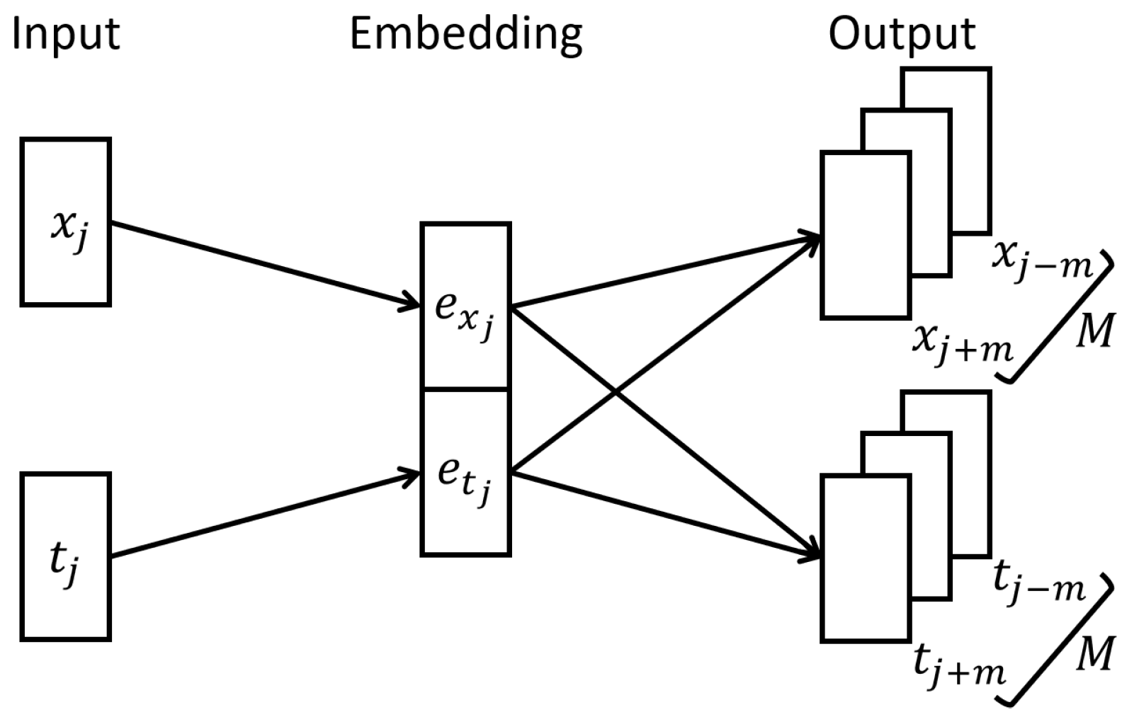
5.2. Creation of Embedding Training Datasets
To train the embedding approach, an embedding training set is required. Therefore, we created trigrams (context
) for all sessions in the training sets. For each interaction
in a session with its corresponding timestamp
a trigram was defined as
. To solve the issue with
, we introduce the “START” and “END” token, which has already been used in the literature [
17,
33,
53].
For T2V the Time2Vec part did not need any form of n-grams. As aforementioned, Time2Vec takes any measure of time as input. For our approach, we utilized the average time delta in seconds for a session since the earliest recorded timestamp in the dataset. To calculate such a time delta for a session, we used and fitted the Time2Vec part of the approach by predicting if the session results in a purchase.
5.3. Embedding Training for Customer Representation
We implemented the three approaches as described in
Section 4 and trained an embedding model accordingly for each of the two splits for all three datasets. Regarding TEE and TEE-CBOW, we split the interaction time
into four time features:
day of the year (dy) to capture patterns on days like Christmas or Black Friday,
day of the week (dw) to capture occurring patterns of certain days of the week,
hour of the day (hd) to capture occurring patterns on the hour of the day, and
minute of the hour (mh) to capture patterns regarding the time within a session. Each of the four time features gets its own embedding
that is concatenated as aforementioned, which results in
. Additionally, to the advantage of identifying and learning recurring time-related patterns, the four time embeddings also mitigate the issue of a potentially extensive one-hot encoding that would arise when using the mere timestamp values.
In the real world, new products and, therefore, interactions are introduced frequently. For our experiments, this is represented by interactions that are in the test set but not in the training set. Embeddings need a predefined number of inputs and inputs that are not among these predefined inputs cannot be handled by the embedding. We need a way to counter the so-called out-of-vocabulary problem. In natural language processing, many approaches were already proposed to solve this problem. We decided to introduce the “Unknown” token, which is one way to deal with the out-of-vocabulary problem [
17,
54]. Therefore, we increased the input layer by one and each unknown interaction of the evaluation will be replaced by this “Unknown” token.
5.4. Baseline Customer Representation
We selected the state-of-the-art approach from Alves Gomes et al. [
17] as a baseline. In their work, customers are represented by an embedding that solely utilizes the interaction context. They utilized a skipgram embedding and have shown in their work that their feature representation combined with an LSTM approach is at least as good as other state-of-the-art approaches and, at the same time, real-time capable. Other approaches, like the one from Esmeli et al. [
14], were also initially tested for our use case but were around 0.1 worse in F1 score and much slower. Hence, we do not consider those approaches further.
5.5. Experiment Evaluation
For evaluation, we use three different approaches. To evaluate the performance of the approach, we use the AUC and the F1 score. To find out if an approach is real-time capable, we measure the time the approach takes to create a customer representation from a session and the time for the LSTM to make a prediction. It is not unusual that a webshop receives thousands of requests per second. In order to evaluate if the approach is real-time capable we implemented two different tests in which a growing amount of sessions needed to be processed and the time it takes was measured. Therefore, we fed n randomly chosen yoochoose sessions to the different approaches and the LSTM and measured the time it took for each n from 1 to , to the power of ten steps. This process was repeated 100 times. The customer representation and the prediction have been evaluated separately because even though we only made the prediction with an LSTM, the prediction architecture might change. The time it took for the LSTM to process the input was only measured once with data embedded with the TEE, as it had the longest vector representation.
6. Results and Discussion
6.1. Prediction Evaluation
Table 4 shows the results of our experiments. It can be seen that our proposed TEE approach is the best-performing one on all datasets and splits. The TEE-CBOW is nearly as good as TEE and slightly better for the yoochoose
last_month split. Especially regarding the yoochoose splits, our proposed TEE approach significantly improved the performance compared to the baselines and T2V. In comparison to the baseline, it resulted in a 0.137 improvement in F1 score and a 0.122 improvement in AUC score for the 20% random split. The
last_month split shows a very similar performance improvement. Regarding the openCDP splits, we see an F1 increase of around 0.03 and an AUC score increase of around 0.02 for both splits. For our own use case, the TEE improved the F1 accuracy and AUC score by around 0.01. The results also show that our proposed T2V approach was the worst-performing approach. For the yoochoose dataset with a
20_percent split, the T2V approach decreased the performance with regard to the AUC score from 0.829 down to 0.816 (−0.013), but increased the F1 score from 0.744 to 0.749 (+0.005). On the
last_month split, the AUC went down to 0.757 (−0.021). The F1 score, on the other hand, rose to 0.708 (+0.028). For the closed dataset, this became even worse. With the
20_percent split, the F1 score changed from 0.890 to 0.878 (−0.012) and the AUC score from 0.94 to 0.925 (−0.015). The performance of the T2V with the
last_month split again decreased the AUC score from 0.868 to 0.864 (−0.004), and the F1 score from 0.922 to 0.913 (−0.009). Lastly, for the openCDP, this behavior stays the same. With a
20_percent split, the F1 score dropped from 0.892 to 0.888 (−0.004), while the AUC score decreased from 0.940 to 0.939 (−0.001). For the
last_month split, the F1 score stayed the same and the AUC score went from 0.948 down to 0.946 (−0.002).
After the evaluation, we can positively answer both of our formulated research questions. With the TEE approach, we were able to include time information in an embedding-based customer representation. Furthermore, the results show that the TEE representation leads to a better customer behavior representation by scoring higher than mere activity embeddings on all three datasets. The same applies to TEE-CBOW. In the conducted experiment, it was only slightly worse than TEE and, therefore, it is also a viable option. For both TEE approaches, we have reasons to assume that the LSTM is able to capture interaction and time patterns from the customer representation. The proposed T2V approach, which combines Time2Vec and an interaction embedding, unfortunately did not lead to any improvement. In most cases, the results were even slightly worse than the baseline embedding approach. This suggests the assumption that the time information from the activities is not represented well by the T2V embedding. The reasons could be that the time and interaction embedding are trained independently of each other and, therefore, the information that is captured in each embedding gets mixed up after the combination of both.
The results not only give an idea about which proposed approach performs best but show several general discoveries. We notice that the baseline approach performs better for the closed and openCDP datasets than for yoochoose. Both openCDP and the closed dataset contain more information regarding customer interactions by adding event type information, which makes it easier for the learning model to predict purchases. For example, sessions without “add to cart” events will not end in a purchase. We investigated this by inserting each customer interaction of a session one-by-one into the used LSTM for our use case. The probability is about 30% after the first interaction and decreases with each additional page visit. However, after the first “add to cart” interaction, the purchase probability of the model increased to about 60%. By adding time to the sessions of these two datasets, which already has indicators in the embedding, we see that it has less impact than adding time information to the sessions of the yoochoose sessions, which do not have additional event information. Therefore, it indicates that adding time information has a larger impact on the performance of interaction embeddings with less additional information as shown in the yoochoose experiments.
Another observation is that due to the two different test splits, it became apparent that each approach performed worse when tested with last month’s data compared to randomly selected test data. Since the model was trained only on data that preceded the test data, it can be argued that the results for the split by last month are more meaningful and closer to a real-life scenario than randomly selecting a percentage of the given data. Not only does this split keep the data in a timely ordered manner. It also lets us assume that users interact in other ways, depending on the time of the year.
6.2. Real-Time Evaluation
Besides the performance evaluation, we also evaluated the time the proposed approaches and the baseline needed to create the customer representation from an ongoing session. Note that the time that TEE takes to embed customer activities is similar to the time TEE-CBOW takes, and therefore, in the following, we only display the measured time for TEE. The results for the real-time evaluation are shown in
Table 5. Each entry of the table is the time it took to create
n user representations in seconds, for
. The entry for the
TEE (mod) represents the time it took the TEE to create a customer representation if the timestamp is already separated into the different time features. For all other approaches, it is the time it took to first process the timestamps, followed by the creation of the representation.
TEE only (mh) only uses a single time feature, in this case "minute of the hour". The table also displays the inference time of the LSTM.
As aforementioned, we defined real time as something that happens within 0.1 s. Our proposed TEE approach can embed around 1770 customer sessions within 0.1 s, which is around five times slower than the baseline that is able to embed almost 8000 customer sessions at the same time. Around 25% of the time TEE takes to embed a customer session is used to compute the time features. Furthermore, the results show that the performance is growing linear to the number of features that should be embedded. This can be derived by comparing the time taken by TEE (mh only) with the baseline and TEE. The baseline only has the interaction features to embed and is around twice as fast as TEE (only mh), which embeds interaction and only one time feature. For a live scenario, the number of embedded time features could be a dynamic parameter based on the number of requests made simultaneously. If the load is high, fewer time features are embedded at the cost of some accuracy. This is a trade-off that needs to be considered and further investigated. The T2V approach takes around 7.7 times as long as the baseline approach. The results also show that the embeddings have a linear time complexity.
It should be noted that all these results are executed without any form of parallelization. Depending on the degree of parallelization, all approaches can operate in real time and process multiple sessions simultaneously. Moreover, interaction embeddings are computed incrementally in a live scenario, rather than all at once in one complete session as in our experimental setup.
6.3. Ablation Studies
In order to evaluate the different used time features on the TEE, we conducted an ablation study, in which we systematically removed time features for the yoochoose dataset.
Table 6 shows the prediction results of the TEE and TEE modifications in which certain time features have been removed. The modifier ‘full’ repeats the best-found performance of the TEE approach without any removed components. For easier comparison, ‘w/o
X’ represents that time feature
X has been removed, and ‘only
X’ means that all time features except
X have been removed. The
Table 6 shows that the time feature mh has the biggest influence on the model’s performance. This is particularly evident in the fact that the performance of the purchase prediction barely degrades when all other time features except mh are removed. This is strengthened by the fact that using only mh as the time feature for TEE reduces the F1 score from 0.881 to 0.86, and removing only the mh information reduces the F1 score from 0.881 to 0.825. Note, we only removed the corresponding embedding part
but used the same hyperparameters as for the full embedding. A new hyperparameter search might lead to the model performing as good or even better than previously.
The results of the ablation study lead to the assumption that the three time features, namely dy, dw, and hd, do not add significant informative content to the embedding. For the dy time feature, the reason could be that the datasets used in our study only have events recorded from several months. Additionally, training paradigms like skipgram or CBOW requires the prediction of the context, but for the dy time features, the context rarely changes. Even though it is possible that this value does change as a session starts before and ends after midnight, this is not the case for most sessions. Naturally, this also holds true for the dw time feature. Similarly, the hd time feature changes only if a session happens between an hour change. This could be used to justify the usefulness of the mh feature for the model’s performance and for the TEE approach as representation. Activities happen within minutes, and this is reflected by the context of the customer activity. In any case, the choice of appropriate time features needs to be examined more in future studies.
7. Summary and Outlook
For online retailers, it is of great importance to know their customers’ intentions. Especially if the customers want to purchase in an ongoing session, which allows the webshop providers to make personalized offers to the customers in real time. We propose a novel time extended embedding approach that encodes customer interactions and the time to represent customer behavior in a session. The representation can be created in real time and is useable for known and unknown customers alike. The embedded interactions are used as input for an LSTM classifier to predict the outcome of the session. Most of the related work requires extensive feature engineering by domain experts to represent customers, which needs to be adjusted for new use cases. In contrast, our approach learns the customer representation from the context of the event data with the power of embeddings and is, therefore, transferable to different use cases without further ado. Furthermore, our proposed representation allows the LSTM to make more accurate predictions than previous approaches. Especially when additional information like event types is not given, our approach can boost the F1 accuracy from 68% to 84%. Despite being more accurate than other state-of-the-art approaches, our approach is around five times slower than mere interaction embeddings. However, our approach is still real-time capable.
Many new open questions remain that we want to address in the future. In a next step, we want to evaluate the TEE approach on other e-commerce tasks, like recommendations and see if it can also improve the recommendation performance. Further, we want to investigate the information amount of the added time features. The results indicate that depending on the initial information content of the interaction, time plays an important or less important role. To this end, we want to examine which information does play an important role in customer representation. The first ablation studies conducted show that the “minute of the hour” feature is the most important feature, with the largest influence on the performance. Also, the fact that other information like the event type has an influence on the performance will be investigated further.
Another future task is to extend the input information for the prediction model. By now, we only utilize the information that could be gathered in a session, but for customers that are known, we can also use historical information. Therefore, we can use the same embedding approach to represent the historical customer sessions. The added time information would enable the model to learn time-relevant patterns, which are useful when using an attention mechanism. For example, a customer is actually a shared family account, and each Friday family member A uses the account and each Tuesday the account is used by family member B. Both of them have different behavior, interests, and therefore, intentions. An attention-based model could learn that on a Friday, family member A’s behavior is relevant and decisive.


