
Delving into Human Factors through LSTM by Navigating Environmental Complexity Factors within Use Case Points for Digital Enterprises


Abstract
:1. Introduction
2. Related Work
3. Methodology
3.1. Dataset Description
3.2. Dataset Pre-Processing
3.3. Model Descriptions
- subsample: denotes the fraction of observations to be randomly sampled for each tree;
- colsample_bytree: the subsample ratio of columns when constructing each tree;
- max_depth: the maximum depth of a tree;
- min_child_weight: defines the minimum sum of weights of all observations required in a child;
- learning_rate: the shrinkage made at every step.
- defining the number of LSTM units;
- defining the number of LSTM layers;
- defining the dropout rate;
- determining LSTM’s time step input.
- learning_rate: the shrinkage made at every step.
3.4. Evaluation Metrics
3.5. Post Agnostic Models: SHAP i LIME
4. Results
5. Discussion
Limitations and Future Directions
6. Conclusions
Author Contributions
Funding
Institutional Review Board Statement
Informed Consent Statement
Data Availability Statement
Conflicts of Interest
References
- Vavpotič, D.; Kalibatiene, D.; Vasilecas, O.; Hovelja, T. Identifying key characteristics of business rules that affect software project success. Appl. Sci. 2022, 12, 762. [Google Scholar] [CrossRef]
- Khan, J.; Jaafar, M.; Mubarak, N.; Khan, A.K. Employee mindfulness, innovative work behaviour, and IT project success: The role of inclusive leadership. Inf. Technol. Manag. 2022, 1–15. [Google Scholar] [CrossRef]
- Marapelli, B.; Carie, A.; Islam, S.M. Software effort estimation with use case points using ensemble machine learning models. In Proceedings of the 2021 International Conference on Electrical, Computer and Energy Technologies (ICECET), Cape Town, South Africa, 9–10 December 2021; pp. 1–6. [Google Scholar] [CrossRef]
- Rankovic, N.; Rankovic, D.; Ivanovic, M.; Lazic, L. A novel UCP model based on artificial neural networks and orthogonal arrays. Appl. Sci. 2021, 11, 8799. [Google Scholar] [CrossRef]
- Rankovic, N.; Rankovic, D.; Ivanovic, M.; Lazic, L. A new approach to software effort estimation using different artificial neural network architectures and Taguchi orthogonal arrays. IEEE Access 2021, 9, 26926–26936. [Google Scholar] [CrossRef]
- Nhung, H.L.T.K.; Van Hai, V.; Silhavy, P.; Prokopova, Z.; Silhavy, R. Incorporating statistical and machine learning techniques into the optimization of correction factors for software development effort estimation. J. Softw. Evol. Process 2023, e2611. [Google Scholar] [CrossRef]
- Silhavy, R. Use Case Points Benchmark Dataset. Mendeley Data V1. 2017. Available online: https://data.mendeley.com/datasets/2rfkjhx3cn/1 (accessed on 1 February 2021).
- Carroll, E.R. Estimating software based on use case points. In Proceedings of the 20th Annual ACM SIGPLAN Conference on Object-Oriented Programming, Systems, Languages, and Applications—OOPSLA ’05, San Diego, CA, USA, 16–20 October 2005; pp. 257–265. [Google Scholar] [CrossRef]
- Nassif, A.B.; Capretz, L.F.; Ho, D. Enhancing Use Case Points Estimation Method using Soft Computing Techniques. J. Glob. Res. Comput. Sci. 2010, 1, 12–21. [Google Scholar]
- Azzeh, M. Fuzzy Model Tree for Early Effort Estimation Machine Learning and Applications. In Proceedings of the 12th International Conference on Machine Learning and Applications, Miami, FL, USA, 4–7 December 2013; pp. 117–121. [Google Scholar] [CrossRef]
- Urbanek, T.; Prokopova, Z.; Silhavy, R.; Sehnalek, S. Using Analytical Programming and UCP Method for Effort Estimation. In Proceedings of the Modern Trends and Techniques in Computer Science; Advances in Intelligent Systems and Computing. Springer: Berlin/Heidelberg, Germany, 2014; Volume 285, pp. 571–581. [Google Scholar] [CrossRef]
- Kaur, A.; Kaur, K. Effort Estimation for Mobile Applications Using Use Case Point (UCP). In Smart Innovations in Communication and Computational Sciences; Springer: Singapore, 2019; pp. 163–172. [Google Scholar] [CrossRef]
- Ani, Z.C.; Basri, S.; Sarlan, A.A. Reusability assessment of UCP-based effort estimation framework using object-oriented approach. J. Telecommun. Electron. Comput. Eng. 2017, 9, 111–114. [Google Scholar]
- Mahmood, Y.; Kama, N.; Azmi, A.A. Systematic review of studies on use case points and expert-based estimation of software development effort. J. Softw. Evol. Process. 2020, 32, e2245. [Google Scholar] [CrossRef]
- Gebretsadik, K.K.; Sewunetie, W.T. Designing Machine Learning Method for Software Project Effort Prediction. Comput. Sci. Eng. 2019, 9, 6–11. [Google Scholar]
- Alves, R.; Valente, P.; Nunes, N.J. Improving software effort estimation with human-centric models: A comparison of UCP and iUCP accuracy. In Proceedings of the 5th ACM SIGCHI Symposium on Engineering Interactive Computing Systems, London, UK, 24–27 June 2013; pp. 287–296. [Google Scholar] [CrossRef]
- Silhavy, R.; Bures, M.; Alipio, M.; Silhavy, P. More Accurate Cost Estimation for Internet of Things Projects by Adaptation of Use Case Points Methodology. IEEE Internet Things J. 2023, 10, 19312–19327. [Google Scholar] [CrossRef]
- Azzeh, M.; Nassif, A.B.; Martín, C.L. Empirical analysis on productivity prediction and locality for use case points method. Softw. Qual. J. 2021, 29, 309–336. [Google Scholar] [CrossRef]
- Pandey, P.; Litoriya, R. Fuzzy Cognitive Mapping Analysis to Recommend Machine Learning-Based Effort Estimation Technique for Web Applications. Int. J. Fuzzy Syst. 2020, 22, 1212–1223. [Google Scholar] [CrossRef]
- Sreekanth, N.; Rama Devi, J.; Shukla, K.A.; Mohanty, D.K.; Srinivas, A.; Rao, G.N.; Alam, A.; Gupta, A. Evaluation of estimation in software development using deep learning-modified neural network. Appl. Nanosci. 2023, 13, 2405–2417. [Google Scholar] [CrossRef]
- Shah, M.A.; Jawawi, D.N.A.; Isa, M.A.; Younas, M.; Abdelmaboud, A.; Sholichin, F. Ensembling Artificial Bee Colony with Analogy-Based Estimation to Improve Software Development Effort Prediction. IEEE Access 2020, 8, 58402–58415. [Google Scholar] [CrossRef]
- Pustejovsky, J.E.; Tipton, E. Meta-analysis with Robust Variance Estimation: Expanding the Range of Working Models. Prev. Sci. 2022, 23, 425–438. [Google Scholar] [CrossRef] [PubMed]
- Khan, M.S.; Jabeen, F.; Ghouzali, S.; Rehman, Z.; Naz, S.; Abdul, W. Metaheuristic Algorithms in Optimizing Deep Neural Network Model for Software Effort Estimation. IEEE Access 2021, 9, 60309–60327. [Google Scholar] [CrossRef]
- Shim, S.R.; Kim, S.J.; Lee, J.; Rücker, G. Network meta-analysis: Application and practice using R software. Epidemiol. Health 2019, 41, e2019013. [Google Scholar] [CrossRef] [PubMed]
- Mahmood, Y.; Kama, N.; Azmi, A.; Khan, A.S.; Ali, M. Software effort estimation accuracy prediction of machine learning techniques: A systematic performance evaluation. Softw. Pract. Exper. 2022, 52, 39–65. [Google Scholar] [CrossRef]
- Gustav, K. Resource Estimation for Objectory Projects; Objective Systems SF AB: Kista, Sweden, 1993; pp. 1–9. [Google Scholar]
- Maja, M.M.; Letaba, P. Towards a data-driven technology roadmap for the bank of the future: Exploring big data analytics to support technology roadmapping. Soc. Sci. Humanit. Open 2022, 6, 100270. [Google Scholar] [CrossRef]
- Maharana, K.; Mondal, S.; Nemade, B. A review: Data pre-processing and data augmentation techniques. Glob. Transit. Proc. 2022, 3, 91–99. [Google Scholar] [CrossRef]
- Chen, D.; Liu, Y.; Huang, L.; Wang, B.; Pan, P. Geoaug: Data augmentation for few-shot nerf with geometry constraints. In European Conference on Computer Vision; Springer: Cham, Switzerland, 2022; pp. 322–337. [Google Scholar] [CrossRef]
- Nielsen, F. Statistical divergences between densities of truncated exponential families with nested supports: Duo Bregman and duo Jensen divergences. Entropy 2022, 24, 421. [Google Scholar] [CrossRef] [PubMed]
- Pei, X.; Zhao, Y.; Chen, L.; Guo, Q.; Duan, Z.; Pan, Y.; Hou, H. Robustness of machine learning to color, size change, normalization, and image enhancement on micrograph datasets with large sample differences. Mater. Des. 2023, 232, 112086. [Google Scholar] [CrossRef]
- Islam, M.J.; Ahmad, S.; Haque, F.; Reaz, M.B.I.; Bhuiyan, M.A.S.; Islam, M.R. Application of min-max normalization on subject-invariant EMG pattern recognition. IEEE Trans. Instrum. Meas. 2022, 71, 1–12. [Google Scholar] [CrossRef]
- Zhang, C.; Zou, X.; Lin, C. Fusing XGBoost and SHAP models for maritime accident prediction and causality interpretability analysis. J. Mar. Sci. Eng. 2022, 10, 1154. [Google Scholar] [CrossRef]
- Zhang, P.; Jia, Y.; Shang, Y. Research and application of XGBoost in imbalanced data. Int. J. Distrib. Sens. Netw. 2022, 18, 15501329221106935. [Google Scholar] [CrossRef]
- Ben Jabeur, S.; Stef, N.; Carmona, P. Bankruptcy prediction using the XGBoost algorithm and variable importance feature engineering. Comput. Econ. 2023, 61, 715–741. [Google Scholar] [CrossRef]
- Li, D.C.; Lin, M.Y.C.; Chou, L.D. Macroscopic big data analysis and prediction of driving behavior with an adaptive fuzzy recurrent neural network on the internet of vehicles. IEEE Access 2022, 10, 47881–47895. [Google Scholar] [CrossRef]
- Tan, K.L.; Lee, C.P.; Anbananthen, K.S.M.; Lim, K.M. RoBERTa-LSTM: A hybrid model for sentiment analysis with transformer and recurrent neural network. IEEE Access 2022, 10, 21517–21525. [Google Scholar] [CrossRef]
- Ariza-Colpas, P.P.; Vicario, E.; Oviedo-Carrascal, A.I.; Butt Aziz, S.; Piñeres-Melo, M.A.; Quintero-Linero, A.; Patara, F. Human activity recognition data analysis: History, evolutions, and new trends. Sensors 2022, 22, 3401. [Google Scholar] [CrossRef] [PubMed]
- Al Hamoud, A.; Hoenig, A.; Roy, K. Sentence subjectivity analysis of a political and ideological debate dataset using LSTM and BiLSTM with attention and GRU models. J. King Saud Univ.-Comput. Inf. Sci. 2022, 34, 7974–7987. [Google Scholar] [CrossRef]
- Wang, F.; Laili, Y.; Zhang, L. Trust Evaluation for Service Composition in Cloud Manufacturing Using GRU and Association Analysis. IEEE Trans. Ind. Inform. 2022, 19, 1912–1922. [Google Scholar] [CrossRef]
- Rankovic, D.; Rankovic, N.; Ivanovic, M.; Lazic, L. The Generalization of Selection of an Appropriate Artificial Neural Network to Assess the Effort and Costs of Software Projects. In IFIP International Conference on Artificial Intelligence Applications and Innovations; Springer International Publishing: Cham, Switzerland, 2022; pp. 420–431. [Google Scholar] [CrossRef]
- Rankovic, D.; Rankovic, N.; Ivanovic, M.; Lazic, L. Convergence rate of Artificial Neural Networks for estimation in software development projects. Inf. Softw. Technol. 2021, 138, 106627. [Google Scholar] [CrossRef]
- Slack, D.; Hilgard, S.; Jia, E.; Singh, S.; Lakkaraju, H. Fooling lime and shap: Adversarial attacks on post hoc explanation methods. In Proceedings of the AAAI/ACM Conference on AI, Ethics, and Society, New York, NY, USA, 7–8 February 2020; pp. 180–186. [Google Scholar] [CrossRef]
- Panati, C.; Wagner, S.; Brüggenwirth, S. Feature relevance evaluation using grad-CAM, LIME and SHAP for deep learning SAR data classification. In Proceedings of the 2022 23rd International Radar Symposium (IRS), Gdansk, Poland, 12–14 September 2022; pp. 457–462. [Google Scholar] [CrossRef]
- Gramegna, A.; Giudici, P. SHAP and LIME: An evaluation of discriminative power in credit risk. Front. Artif. Intell. 2021, 4, 752558. [Google Scholar] [CrossRef] [PubMed]
- Holzinger, A.; Saranti, A.; Molnar, C.; Biecek, P.; Samek, W. Explainable AI methods-a brief overview. In xxAI-Beyond Explainable AI: International Workshop, Held in Conjunction with ICML 2020, Vienna, Austria, 18 July 2020, Revised and Extended Papers; Springer International Publishing: Cham, Switzerland, 2022; pp. 13–38. [Google Scholar] [CrossRef]
- Sahay, S.; Omare, N.; Shukla, K.K. An Approach to identify Captioning Keywords in an Image using LIME. In Proceedings of the 2021 International Conference on Computing, Communication, and Intelligent Systems (ICCCIS), Greater Noida, India, 19–20 February 2021; pp. 648–651. [Google Scholar] [CrossRef]
- Ye, X.; Fang, F.; Wu, J.; Bunescu, R.; Liu, C. Bug Report Classification Using LSTM Architecture for More Accurate Software Defect Locating. In Proceedings of the 2018 17th IEEE International Conference on Machine Learning and Applications (ICMLA), Orlando, FL, USA, 17–20 December 2018; pp. 1438–1445. [Google Scholar] [CrossRef]
- Dam, H.K.; Tran, T.; Pham, T.; Ng, S.W.; Grundy, J.; Ghose, A. Automatic Feature Learning for Predicting Vulnerable Software Components. IEEE Trans. Softw. Eng. 2021, 47, 67–85. [Google Scholar] [CrossRef]
- Stach, W.; Pedrycz, W.; Kurgan, L.A. Learning of Fuzzy Cognitive Maps Using Density Estimate. IEEE Trans. Syst. Man Cybern. Part B Cybern. 2012, 42, 900–912. [Google Scholar] [CrossRef] [PubMed]
- Sharma, A.; Tselykh, A. Machine Learning-Enabled Estimation System Using Fuzzy Cognitive Mapping: A Review. In Proceedings of Third International Conference on Computing, Communications, and Cyber-Security; Singh, P.K., Wierzchoń, S.T., Tanwar, S., Rodrigues, J.J.P.C., Ganzha, M., Eds.; Lecture Notes in Networks and Systems; Springer: Singapore, 2023; Volume 421. [Google Scholar] [CrossRef]


| Feature Name UCP Model | Original Type | Description |
|---|---|---|
| Unadjusted Actor Weight (UAW) | Numerical | Point size of the software that accounts for the number and complexity of actors |
| Unadjusted Use Case Weight (UUCW) | Numerical | Complexity and size of the use cases |
| Unadjusted Use Case Point (UUCP) | Numerical | Unadjusted use case point |
| Technical Complexity Factor (TCF) | Numerical | Factor that is used to adjust the size based on technical considerations |
| Environmental Complexity Factor (ECF) | Numerical | Factor that is used to adjust the size based on the considerations |
| Adjusted Use Case Point (AUCP) | Numerical | Adjusted use case point |
| Factor | Description | Weight | Assigned Value | Weight × Assigned Value |
|---|---|---|---|---|
| E1 | Compliance with the used development process | 1.5 | 3 | 4.5 |
| E2 | Experience with applications | 0.5 | 3 | 1.5 |
| E3 | Team experience with technologies | 1.0 | 3 | 2 |
| E4 | Capabilities of the chief analyst | 0.5 | 5 | 2.5 |
| E5 | Team motivation | 1.0 | 2 | 2 |
| E6 | Stability of requirements | 2.0 | 1 | 2 |
| E7 | Part-time staff | −1.0 | 0 | 0 |
| E8 | Programming language complexity | −1.0 | 4 | −4 |
| Total (EF): | 10.5 | |||
| Datasets | ECF | N | Min Value | Max Value | Mean | Standard Deviation |
|---|---|---|---|---|---|---|
| Dataset_1 | [0.71; 1.08] | 50 | 5775.0 | 7920.0 | 6506.9 | 653.0 |
| Dataset_2 | [0.94; 1.12] | 21 | 6162.6 | 6525.3 | 6393.9 | 118.2 |
| Dataset_3 | [0.71; 1.12] | 18 | 2692.1 | 3246.6 | 2988.4 | 233.2 |
| Dataset_4 | [0.71; 1.08] | 17 | 2176.0 | 3216.0 | 2589.4 | 352.1 |
| Datasets | ECF | N | Min Value | Max Value | Mean | Standard Deviation |
|---|---|---|---|---|---|---|
| Dataset_1 | [0.57; 1.08] | 648 | 4892.3 | 6548.1 | 5402.5 | 538.2 |
| Dataset_2 | [0.94; 1.08] | 216 | 5430.7 | 7123.4 | 6208.4 | 456.7 |
| Dataset_3 | [0.71; 1.12] | 108 | 43,890.4 | 6291.3 | 5467.8 | 652.9 |
| Dataset_4 | [0.57; 1.08] | 108 | 2856.7 | 4775.6 | 3818.9 | 438.0 |
| Models | Training | Testing | Validation1 | Validation2 | ||||
|---|---|---|---|---|---|---|---|---|
| MRE | MSE | MRE | MSE | MRE | MSE | MRE | MSE | |
| XGBoost | 0.935 | 252.29 | 0.915 | 257.80 | 0.923 | 255.57 | 0.931 | 253.37 |
| Taguchi method | 0.933 | 252.82 | 0.929 | 253.92 | 0.920 | 256.40 | 0.917 | 257.24 |
| LSTM | 0.983 | 239.98 | 0.992 | 236.84 | 0.984 | 239.73 | 0.980 | 240.70 |
| GRU | 0.971 | 242.94 | 0.980 | 240.70 | 0.973 | 242.44 | 0.968 | 243.69 |
| MMRE | 0.955 | 0.954 | 0.950 | 0.949 | ||||
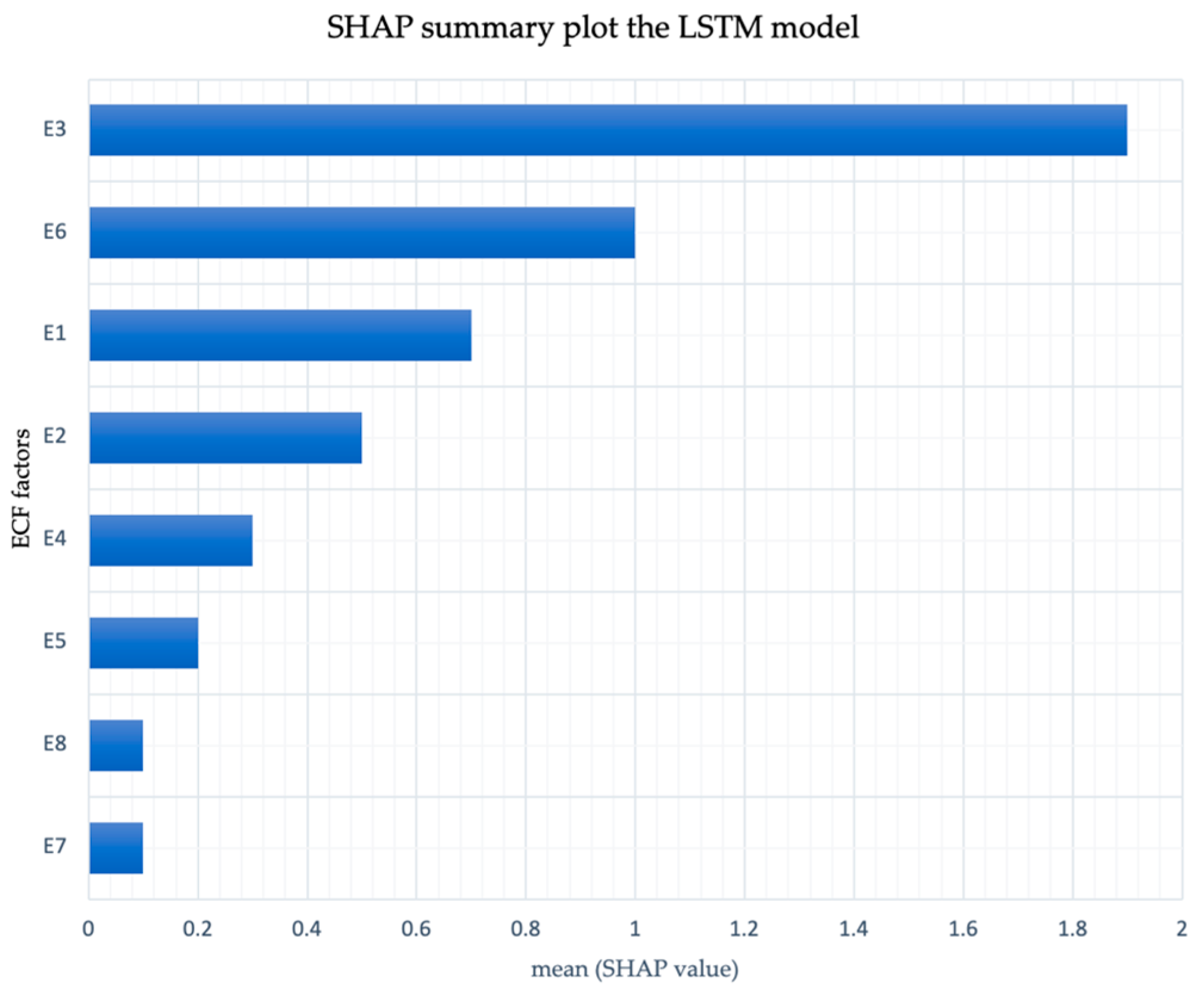
| ECF Factors | Training | Testing | Validation1 | Validation2 | Total |
|---|---|---|---|---|---|
| δD1 | δD2 | δD3 | δD4 | δD5 | |
| E1 | 0.7 | 0.6 | 0.7 | 0.6 | 0.7 |
| E2 | 0.5 | 0.5 | 0.5 | 0.6 | 0.5 |
| E3 | 1.7 | 1.8 | 1.9 | 2.0 | 1.9 |
| E4 | 0.2 | 0.3 | 0.4 | 0.4 | 0.3 |
| E5 | 0.1 | 0.2 | 0.3 | 0.2 | 0.2 |
| E6 | 0.9 | 1.0 | 1.1 | 1.2 | 1.0 |
| E7 | 0.1 | 0.1 | 0.1 | 0.1 | 0.1 |
| E8 | 0.1 | 0.2 | 0.1 | 0.1 | 0.1 |
| Total | 4.3 | 4.7 | 5.1 | 5.2 | 4.8 |
Disclaimer/Publisher’s Note: The statements, opinions and data contained in all publications are solely those of the individual author(s) and contributor(s) and not of MDPI and/or the editor(s). MDPI and/or the editor(s) disclaim responsibility for any injury to people or property resulting from any ideas, methods, instructions or products referred to in the content. |
© 2024 by the authors. Licensee MDPI, Basel, Switzerland. This article is an open access article distributed under the terms and conditions of the Creative Commons Attribution (CC BY) license (https://creativecommons.org/licenses/by/4.0/).
Share and Cite
Rankovic, N.; Rankovic, D. Delving into Human Factors through LSTM by Navigating Environmental Complexity Factors within Use Case Points for Digital Enterprises. J. Theor. Appl. Electron. Commer. Res. 2024, 19, 381-395. https://doi.org/10.3390/jtaer19010020
Rankovic N, Rankovic D. Delving into Human Factors through LSTM by Navigating Environmental Complexity Factors within Use Case Points for Digital Enterprises. Journal of Theoretical and Applied Electronic Commerce Research. 2024; 19(1):381-395. https://doi.org/10.3390/jtaer19010020
Chicago/Turabian StyleRankovic, Nevena, and Dragica Rankovic. 2024. "Delving into Human Factors through LSTM by Navigating Environmental Complexity Factors within Use Case Points for Digital Enterprises" Journal of Theoretical and Applied Electronic Commerce Research 19, no. 1: 381-395. https://doi.org/10.3390/jtaer19010020