Analysis of Longitudinal Guided Wave Propagation in a Liquid-Filled Pipe Embedded in Porous Medium

Abstract

To study the leakage situation of a liquid-filled pipe in long-term service, a model of a liquid-filled pipe embedded in an infinite porous medium as well as in a finite porous medium is designed. The principal motivation is to perform detailed quantitative analysis of the longitudinal guided wave propagating in a liquid-filled pipe embedded in a saturated porous medium. The problems of pipeline leakage and porosity as well as the media outside the pipe are solved to identify the characteristics of the guided wave in a more practical model. The characteristics of the guided wave are investigated theoretically and numerically, with special emphasis on the influence of porous medium parameters on the dispersion properties. Assuming the pipe is a cylindrical shell buried in an isotropic, homogeneous, and porous medium, the dispersion equations are established based on the elastic-dynamic equations and the modified Biot liquid-saturated porous theory. The characteristics of dispersion, time-domain waveform and attenuation curves varying with porous medium parameters, wrapping layer material, and thickness, are all analyzed. The increase in porosity decreases the partial mode phase velocity in the liquid-filled pipe embedded in the finite porous medium. The characteristics of attenuation are in good agreement with the dispersion curves and the time-domain waveform results.

1. Introduction

Longitudinal ultrasonic guided waves in pipes are widely employed in pipeline detection, as well as pipe condition assessment and monitoring, owing to their long-range propagation and low energy dissipation. The theoretical background of guided waves was first described by a characteristic frequency equation in 1959 [1]. Nondestructive testing that employs guided waves has widespread applications. An example is pipeline corrosion, which is a major problem in the chemical and oil industries. Moreover, there is significant interest in reducing leakage due to corrosion in liquid-filled pipes [2,3,4,5,6,7]. That is, if pipes are filled with a liquid, then ruptures of the wall can generate acoustic waves in the low audio frequency range, which can then be detected by the remote monitoring equipment placed in the fluid or on the walls [8,9]. These detection techniques rely on the propagation of acoustic energy in both the structure and the fluid, as well as the detection and interpretation of energy transfer. However, it is common for these pipes to also be buried underground, or immersed in a fluid, and this can significantly affect the propagation of energy. This often leads to a reduction in the effectiveness of detection techniques, and so it is important to develop a good understanding of the parameters and acoustic propagation characteristics of the media outside the pipe if one is to develop reliable inspection methodologies, particularly when there is an existing leakage in the pipeline.

To clearly describe the physical behavior of a cylindrical wave, many efforts have been devoted to investigating the ultrasonic guided waves. Sinha et al. [10] studied the propagation characteristics of axisymmetric waves in cylindrical shells immersed in liquid and calculated the dispersion curves of the medium wave, which were consistent with experimental results. Lafleur et al. [11] employed both numerical and experimental methods to study the propagation characteristics of axisymmetric guided waves in liquid-filled elastic tubes. They found at least two modes of propagation in an elastic shell at any frequency. Based on the fluid model, Aristégui et al. [12] studied the propagation characteristics of guided waves in a tube, and discussed the differences between complex frequency and complex wave number solutions. Long et al. [13] focused on the attenuation characteristics of the basic mode of propagation in buried pipes. Siqueira et al. [14] combined the ultrasonic guided wave with the wavelet analysis to study the influence of a crack on the propagation of an ultrasonic waveguide in the pipeline. Leinov et al. [15] experimentally investigated the propagation characteristics of guided waves in buried pipelines and analyzed the influence of the variability of soil conditions on the attenuation characteristics of guided waves. Cui et al. [16] conducted a theoretical and numerical investigation of the influence of the contained liquid on backward waves and associated zero-group-velocity modes.

In the above-mentioned references, the predictions presented so far assume that the medium surrounding the pipe is perfect and elastic. It is, however, well known that materials such as soil have internal damping present within their structure, and that this may affect the propagation of an elastic wave. Damping will affect the attenuation of a particular eigenmode, and the effect of the material damping may dominate the attenuation caused by the energy radiating away from a structure [17,18]. Hydrogeological studies also indicate that the medium outside the pipe has a certain complexity, and the shallow surface of the earth is highly porous; thus, it is impractical to apply the elastic medium directly in pipeline detection. Considering that the porous medium takes into account both solid matrix and pore fluid, the porous medium model is more practical and appropriate. Few studies exist on the correlation of pore parameters with pipeline leak detection and precision measurement for saturated porous media, and most have been undertaken in the field of logging [19,20,21,22]. A detailed quantitative analysis of the longitudinal guided wave propagating in a liquid-filled pipe embedded in saturated porous medium is lacking.

In this study, we performed a rigorous mathematical analysis of the longitudinal guided wave propagating in a liquid-filled pipe embedded in infinite and finite porous medium, while considering the influence of the thickness of the medium outside the pipe, which cannot be ignored in the numerical simulation and analysis. The dispersion equations of the longitudinal guided wave are deduced based on the theory of elastic dynamics. The effects of the outer medium were investigated by considering a water-filled pipe embedded in elastic or porous medium. The dispersion characteristics of the water-filled pipe embedded in finite porous medium were computed and compared with the water-filled pipe embedded in infinite porous medium. To observe the dispersion characteristics of guided waves in the liquid-filled pipe system intuitively, the time-domain waveforms at the liquid–pipe interface in the infinite porous medium and at the external interface of the finite porous medium were inverted. Finally, we used the attenuation to interpret the effect of porosity on the guided wave in the liquid-filled pipe embedded in porous medium.

2. Basic Equations and Problem Formulation

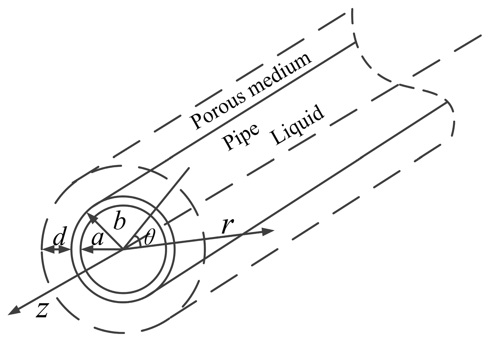
2.1. Geometric Model

Considering the geometrical characteristics of the liquid-filled pipe, this study investigates the longitudinal guided wave propagation characteristics of a liquid-filled pipe embedded in porous medium in cylindrical coordinates $(r,z,\theta )$. The geometry of the problem is illustrated in Figure 1. The z-axis is along the symmetric axis of the pipe, and the inner and outer radii of the metal pipe are a and b. The pipe is filled with liquid, and the outermost layer is a porous medium with a thickness of d. The length of the pipe is assumed to be infinite, and the radial direction of the porous medium can be infinite or finite. Here, three sets of subscripts are adopted to identify a larger number of parameter properties. The first set of subscripts L, E, P, and S represent the liquid, elastic pipe, porous medium, and solid matrix, respectively; the second set of subscripts l and t indicate longitudinal and transverse waves, respectively; the third set of subscripts f and s indicate fast and slow waves in porous medium; $c_{El}$, $c_{Et}$, and ${\rho }_E$ represent the longitudinal wave velocity, transverse wave velocity, and density of the internal elastic pipe, respectively. $c_{Plf}$, $c_{Pls}$, and $c_{Pt}$ denote the fast longitudinal, slow longitudinal, and shear wave velocity in porous medium. The parameters ${\rho }_S$ and ${\rho }_L$ denote the density of the porous medium’s solid skeleton and fluid, respectively, while $c_L$ represents the longitudinal wave velocity in the fluid.

2.2. Dispersion Equations

A symmetrical geometric model (Figure 1) is constructed to derive the dispersion equation. The media in the model are considered to be homogeneous and isotropic. In this subsection, we provide in detail the process used to derive the dispersion equation for axisymmetric modes with the circumferential number n = 0 in a liquid-filled pipe embedded in porous medium. The potential function of this problem is divided into three parts: the pipe, the liquid in the pipe, and the porous medium.

For the elastic medium pipe, the displacement field $\mathsf{u}$ is decomposed into scalar $\Phi$ and vector potential $\mathsf{\Psi }$ with $\nabla \cdot \mathsf{\Psi }=0$,

$$\mathsf{u}=\nabla \Phi +\nabla \times \mathsf{\Psi }$$

(1)

Because of the axisymmetry of the studied modes, the radial and axial components of the vector potential $\mathsf{\Psi }$ are zero, and only the circumferential component ${\Psi }_{\theta }$ is retained [23,24,25,26,27]. The expressions for $\Phi$ and ${\Psi }_{\theta }$ are given by

$$\Phi =\left(A_1{H}_0^1({\alpha }_{1}r)+A_2{H}_0^2({\alpha }_{1}r)\right)\exp [i(kz-\omega t)]$$

(2)

$${\Psi }_{\theta }=\left(B_1{H}_1^1({\beta }_{1}r)+B_2{H}_1^2({\beta }_{1}r)\right)\exp [i(kz-\omega t)]$$

(3)

where ${\alpha }_1^2=k^2-{\omega }^2/c_{El}^2$, ${\beta }_1^2=k^2-{\omega }^2/c_{Et}^2$, k is the number of waves, w is the angular frequency, and A₁, A₂, B₁, and B₂ are the undetermined coefficients. $H_n^{(1)}$ and $H_n^{(2)}$ denote the Hankel functions of the first and second order (n = 0, 1), which can be expressed as a linear combination of Bessel functions and describe the two-dimensional cylindrical wave solution [28]. The displacement expressions of the pipe are respectively given as

$$u_{rE}=\frac{\partial \Phi }{\partial r}-\frac{\partial {\Psi }_{\theta }}{\partial z}$$

(4)

$$u_{zE}=\frac{\partial \Phi }{\partial z}+\frac{1}{r}\frac{\partial (r{\Psi }_{\theta })}{\partial r}$$

(5)

where $\lambda$ and $\mu$ are the Lame constants in the elastic medium. For the inviscid liquid in the pipe, the displacement and stress expression are respectively expressed as

$$u_{rL}=-B_3{\alpha }_L{J}_1({\alpha }_{L}r)\exp [i(kz-\omega t)]$$

(6)

$${\sigma }_{rrL}=-B_3{\lambda }_L{J}_0({\alpha }_{L}r)[k^2+{({\alpha }_L)}^2]\exp [i(kz-\omega t)]$$

(7)

where ${\alpha }_L^2=k^2-{\omega }^2/c_L^2$, ${\lambda }_L={\rho }_L{c}_L^2$, and ${\lambda }_L$ is the Lame constant in the liquid. B₃ is the undetermined coefficient to be determined by boundary conditions. $J_0$ is a modified Bessel function of the first kind.

The thickness of the wrapping layer is not included in the study of the influence of the nondestructive testing parameters. However, sometimes, thickness also plays a very important role in the subsequent numerical simulation and analysis. Therefore, it is necessary to discuss the case of the porous medium being finite. In contrast to other media, the potential function of the porous medium includes both solid and liquid phases. The solid phase has three potential functions describing the fast longitudinal, slow longitudinal, and shear waves. Thus, the wave motion equations based on the framework of the Biot theory modified by Johnson for the scalar potentials are given as [29]

$${\Phi }_{PSlf}=\left(D_1{K}_0\left({\alpha }_{21}r\right)+F_1{I}_0\left({\alpha }_{21}r\right)\right)\exp [i(kz-\omega t)]$$

(8)

$${\Phi }_{PSls}=\left(D_2{K}_0\left({\alpha }_{22}r\right)+F_2{I}_0\left({\alpha }_{22}r\right)\right)\exp [i(kz-\omega t)]$$

(9)

$${\Psi }_{PSt}=\left(D_3{K}_0\left({\beta }_{21}r\right)+F_3{I}_0\left({\beta }_{21}r\right)\right)\exp [i(kz-\omega t)]$$

(10)

where the longitudinal wave potential function ${\Phi }_{PSl}={\Phi }_{PSlf}+{\Phi }_{PSls}$, ${\alpha }_{21}^2=k^2-k_{p1}^2$, ${\alpha }_{22}^2=k^2-k_{p2}^2$, and ${\beta }_{21}^2=k^2-k_t^2$, and D₁, D₂, D₃, F₁, F₂, F₃ are the undetermined coefficients. I₀ is the zero-order Bessel function of the first kind of virtual quantities, which describes the reflection field from the interface. K₀ is the Bessel function of the second kind of the zero-order virtual component, which represents the wave propagating from the acoustic excitation source to infinity.

Three kinds of wave modes with different velocities are obtained in a homogeneous porous medium: a shear wave and two longitudinal waves, often referred to as the fast and slow waves, respectively. In the case of the fast wave, the skeletal frame and the pore fluid move in-phase. This wave is similar to the longitudinal wave in an elastic solid medium. In the case of the slow wave, the frame and the fluid move relative to each other in antiphase. This wave is unique to Biot’s model and all similar porous models. Their wave numbers are $k_{PSlf}=\omega s_{PSlf}$, $k_{PSls}=\omega s_{PSls}$, and $k_{PSt}=\omega s_{PSt}$, respectively. Here, $\omega$ is the angular frequency, and $s_{PSlf}$, $s_{PSls}$, $s_{PSt}$ can be written as

$$s_{PSlf,PSls}^2=\frac{2({\rho }_s{\rho }_L-{\rho }_s{\rho }_{12}-{\rho }_L{\rho }_{12})}{\Delta \pm \sqrt{{\Delta }^2-4({\rho }_s{\rho }_L-{\rho }_s{\rho }_{12}-{\rho }_L{\rho }_{12})(PR-Q^2)}}$$

(11)

$$s_{PSt}^2=\frac{{\rho }_s{\rho }_L-{\rho }_s{\rho }_{12}-{\rho }_L{\rho }_{12}}{N({\rho }_L-{\rho }_{12})}$$

(12)

where $\Delta =P({\rho }_f-{\rho }_{12})+R({\rho }_s-{\rho }_{12})-2{\rho }_{12}Q$, $P=A+2N$, and ${\rho }_{12}$ is the coupling density of the solid and liquid. A, N, R, and Q are all poroelastic constants [30,31]. The poroelastic constants A and N correspond to the familiar Lame constants of a purely elastic solid, and the constant N also represents the shear modulus of the solid. The constant R is a measure of the pressure required on the liquid to force a certain amount into the aggregate, while the total volume remains constant. The constant Q represents the coupling between the volume change of the solid and that of the liquid. The calculated parameters in the porous medium are

$$A=\frac{(1-\beta )(1-\beta -K_{Pb}/K_{PS})K_{PS}+\beta K_{Pb}(K_{PS}/K_{PL})}{1-\beta -K_{Pb}/K_{PS}+\beta (K_{PS}/K_{PL})}-\frac{2}{3}N$$

(13)

$$R=\frac{{\beta }^2{K}_{PS}}{1-\beta -K_{Pb}/K_{PS}+\beta (K_{PS}/K_{PL})}$$

(14)

$$Q=\frac{(1-\beta -K_{Pb}/K_{PS})\beta K_{PS}}{1-\beta -K_{Pb}/K_{PS}+\beta (K_{PS}/K_{PL})}$$

(15)

where K_PS, K_PL, and K_Pb are the bulk moduli of the solid matrix, fluid, and solid skeleton, respectively, while N and $\beta$ denote the shear modulus and porosity in porous medium. With regard to the liquid phase in a porous medium, the equation consists of two parts, namely the longitudinal and the shear wave potential function,

$${\Phi }_{PLl}={\eta }_1{\Phi }_{PSlf}+{\eta }_2{\Phi }_{PSls}$$

(16)

$${\Psi }_{PLt}={\eta }_3{\Psi }_{PSt}$$

(17)

where ${\eta }_1$, ${\eta }_2$, and ${\eta }_3$ are the participation coefficients of the fast longitudinal wave, slow longitudinal wave and shear wave, respectively [32,33].

According to Biot, a porous medium may be considered as a porous skeletal frame that is permeated by a fluid. Biot’s equations quantify the momentum balance within the skeletal frame, within the pore fluid, and between them. It can be shown that as porosity tends to zero, Biot’s equations reduce to the wave equation of a solid, and conversely, as the porosity tends to 1, they reduce to the wave equation of a fluid. The displacement of the porous medium is composed of two basic components: solid displacement and pore fluid displacement.

For the porous medium, the solid displacement and pore fluid displacement are expressed using potential functions as

$$u_{rPS}=\frac{\partial {\Phi }_{PSl}}{\partial r}+\frac{{\partial }^2{\Psi }_{PSt}}{\partial r\partial z}$$

(18)

$$u_{zPS}=\frac{\partial {\Phi }_{PSl}}{\partial z}-\frac{{\partial }^2{\Psi }_{PSt}}{\partial r^2}-\frac{1}{r}\frac{\partial {\Psi }_{PSt}}{\partial r}$$

(19)

$$u_{rPL}=\frac{\partial {\Phi }_{PLl}}{\partial r}+\frac{{\partial }^2{\Psi }_{PLt}}{\partial r\partial z}$$

(20)

$$u_{zPL}=\frac{\partial {\Phi }_{PLl}}{\partial z}-\frac{{\partial }^2{\Psi }_{PLt}}{\partial r^2}-\frac{1}{r}\frac{\partial {\Psi }_{PLt}}{\partial r}$$

(21)

Thus, the boundary conditions are given as follows.

(1) We consider an inviscid liquid, where the liquid–internal tube interface conditions are such that the radial displacement and normal stress components at the boundary are continuous, and the shear stress components are zero at the interface [34]. That is, the boundary conditions at r = a are

$$u_{rE}=u_{rL}$$

(22)

$${\sigma }_{rrE}={\sigma }_{rrL}$$

(23)

$${\sigma }_{rzE}=0$$

(24)

(2) Owing to the impermeability of the elastic solid, the fluid in the porous medium is confined to flowing out at the boundary, such that the displacement of the fluid is equal to that of the solid phase skeleton [35]. The pipe–porous medium interface conditions state that the displacement and stress components at the boundary must be continuous. That is, the boundary conditions at r = b are

$$u_{rE}=(1-\beta )u_{rPs}+\beta u_{rPL}$$

(25)

$$u_{zE}=u_{zPs}$$

(26)

$${\sigma }_{rrE}={\sigma }_{rrPs}+{\sigma }_{rrPL}$$

(27)

$${\sigma }_{rzE}={\sigma }_{rzPs}$$

(28)

$$u_{rPs}=u_{rPL}$$

(29)

(3) It is further assumed that the porous medium layer is finite in a vacuum. Thus, all the stress components are equal to zero at the outer surface of the porous medium layer, i.e., the boundary conditions at r = b + d can be written as

$${\sigma }_{rzPs}=0$$

(30)

$${\sigma }_{rrPL}=0$$

(31)

$${\sigma }_{rrPs}=0$$

(32)

The substitution of Equations (2)–(21) into the boundary conditions (22)–(32) results in a system of linear homogeneous equations in the eleven constants A₁, A₂,…, F₁, F₂, and F₃.

$$\mathbf{M}{(A_1{A}_2{B}_1{B}_2{B}_3{D}_1{D}_2{D}_3{F}_1{F}_1{F}_1)}^T=0$$

(33)

where $\mathbf{M}$ is a 11 × 11 matrix, and the elements m₁₁, …, m₁₁₁₁ are listed in the Appendix A. Equation (33) has non-zero solutions, the coefficient determinant of the equation must be zero, and the corresponding dispersion equation can be obtained as

$$\det (\mathbf{M})=0$$

(34)

When the thickness of the porous medium layer d approaches infinity, the coefficients F₁, F₂, and F₃ would approach zero, as the sound field approaches zero at infinity. The unknown coefficients are reduced to eight in the infinite porous medium. Along similar lines, Equations (2)–(21), along with (22)–(29), yield a system of linear non-homogeneous equations for the axially symmetric vibrations of a liquid-filled pipe embedded in infinite porous medium. The dispersion Equation (34) degenerates to

$$\det ({\mathbf{M}}^{\prime })=0$$

(35)

where ${\mathbf{M}}^{\prime }$ is an 8 × 8 matrix, and the elements m₁₁, …, m₈₈ are the same as in Equation (33).

2.3. Theoretical Verification

In this subsection we validate the formulation developed in this paper with results from the published literature. The purpose of the comparison is to demonstrate the accuracy of the dispersion equations of the model.

To demonstrate the accuracy of the statements of the sound field and the establishment of the dispersion equations, the porosity of porous medium $\beta$ was set to zero. By Equations (11) and (12), we can conclude that the fast longitudinal wave velocity $c_{Plf}$ and the shear wave velocity $c_{Pls}$ are the longitudinal wave velocity and shear wave velocity of the solid skeleton in porous medium, and the slow longitudinal wave velocity $c_{Pt}$ is 0. The slow longitudinal wave does not exist, and so the liquid participation coefficients η₁, η₂ and η₃ are all 0, and the liquid phase potential function is 0. When the porosity is 0, $K_{PS}=K_{Pb}$($K_{PS}$,$K_{Pb}$ are the bulk modulus of the solid skeleton and the bulk modulus of the solid matrix), $N={\mu }_S$. From Equations (13)–(15), $A=K_{PS}-\frac{2}{3}N={\lambda }_S$, $R=0$, $Q=0$, and ${\lambda }_S$ and ${\mu }_S$ are the lame constants of the solid in porous medium. It can be seen that the expressions of displacement and stress, and the boundary conditions, correspond to those in a situation wherein the medium surrounding the liquid-filled pipe is a completely homogeneous elastic medium, and the dispersion equation also satisfies this condition [36,37].

All these prove that when the porous medium becomes a completely homogeneous elastic medium, the statements of the sound field and the dispersion equations satisfy this condition.

In the cylindrical structure with porous media, the dispersion function of the guided wave is a complex function. Equations (34) and (35) represent the relationship between frequencies and wavenumbers, leading to a theoretical zero-problem. By solving Equations (34) and (35), the velocities of the guided wave can be obtained. The real part represents the wave mode information that can be used to plot the phase velocity dispersion curves, and the imaginary part corresponds to the attenuation coefficient.

3. Results and Discussion

The numerical results illustrating the theory derived in the previous section are presented in this section. The main discussion involves the effects of the wrapping layer material, thickness, and the pore parameters on the propagation characteristics of the guided waves. The time-domain waveforms of guided waves are obtained by numerical inversion, and the influences of pore parameters on these waveforms and attenuation coefficients are simulated. Considering the structure of a liquid-filled pipe embedded in porous medium, the relevant parameters selected for numerical simulations are shown in

Table 1. Material properties and geometrical parameters for a case study of a liquid-filled pipe embedded in a porous medium. The pipe fluid and pore fluids are water, and the internal and external pipe radii are a = 14 mm and b = 16 mm.

Material		Density (kg/m3)	Longitudinal Velocity (m/s)	Shear Velocity (m/s)
Pipe		7800	4100	2100
Porous medium	solid skeleton Pore fluid	2700	5370	3100
		998	1483
Water		998	1483

and

Table 2. Material properties of saturated porous medium at porosity $\beta =0.1$.

Parameter	Simulation Value
Pore curvature ${\alpha }_{\infty }$	5.5
Static permeability κ0	1.0 × 10−12 m2
Viscous coefficient n	0.001 kg/(s·m)
Bulk modulus of fluid KPL	2.19 GPa
Bulk modulus of solid skeleton KPb	33.70 GPa
Shear modulus of solid skeleton N	20.86 GPa
Bulk modulus of solid matrix KPS	43.33 GPa

[38,39]. This study focuses on guided waves in a liquid-filled pipe of 14 mm internal and 16 mm external radii.

3.1. Results for Time-Frequency-Domain

The numerical search algorithm has been used to numerically solve the transcendental equations to yield the roots of the dispersion equation [40]. In the layered structure with porous medium, the dispersion function of the guided wave is a complex function. For any given frequency, the corresponding wavenumber is also complex. The real part corresponds to the phase velocity. In this subsection, we validate the formulation developed in this study with results from the elastic medium model. The purpose of the comparison is to demonstrate the accuracy and efficiency of the proposed approach. Two models are chosen: (i) a water-filled pipe embedded in infinite medium, and (ii) a water-filled pipe embedded in finite porous medium.

3.1.1. Water-Filled Pipe in Infinite Porous Medium

Using the parameters listed in Table 1 and Table 2, the expressions in (35) are numerically calculated to obtain roots that correspond to the propagating modes. The water-filled pipe’s internal and external radii are a = 14 mm and b = 16 mm, respectively. The dispersion curves of the longitudinal modes in the water-filled pipe embedded in an infinite porous medium are presented in Figure 2.

This study follows the mode classification of Marston [41]. The longitudinal modes of the liquid-filled pipe’s forward propagation in an infinite porous medium are denoted as L(0,m), where L represents the axisymmetric longitudinal modes with circumferential order n = 0 and mode order m = 1, 2, 3,…. The fundamental modes (i.e., those propagating at zero frequency) are given the value of m = 1, and the higher order modes are numbered consecutively.

For clarity, in Figure 2, we compare the dispersion curves of the water-filled pipe embedded in elastic and porous media. Blue and red lines represent the propagating modes in the water-filled pipe embedded in infinite elastic and porous media, respectively. No porous medium is present outside the pipe, but it is used to validate the dispersion characteristics of guided waves in a water-filled pipe embedded in an infinite porous medium ($\beta$ = 0), and the choice of parameters. The longitudinal and shear velocities, and the density of the elastic medium, are taken to be 5370, 3100 m/s, and 2700 kg/m³, respectively; for the water-filled pipe, the longitudinal and shear velocities and the density are 4100, 2100 m/s, and 7800 kg/m³, respectively, and its internal and external radii are 14 mm and 16 mm, respectively.

Figure 2 shows that in the frequency range f < 0.5 MHz, the longitudinal modes of the water-filled pipe in infinite porous medium comprise eight modes L(0,m) (m = 1, 2, 3, …, 8) and one α mode. The bottom red line represents the α mode in the liquid of the pipe, whose phase velocity is similar to the Scholte wave, and which increases with frequency and gradually tends to a value of 1500 m/s [12]. The remaining red lines depict the longitudinal guided waves of the water-filled pipe in elastic medium. Each exists in a wide frequency range. More specifically, the axisymmetric longitudinal guided waves exist in numerous modes. There is more than one mode at any frequency, and the characteristics of each mode are unique. The longitudinal guided wave velocities in a water-filled pipe embedded in infinite porous medium decrease as a function of the frequency, and slope downward, approaching the longitudinal wave velocity of the liquid in the pipe [42].

The phase velocity and trend of this model are compared to those of the water-filled pipe in the elastic medium model. Figure 2 shows that the phase velocity of the water-filled pipe embedded in elastic medium is slightly lower than the phase velocity of the water-filled pipe embedded in a porous medium, and the trend of changes in the water-filled pipe is consistent in both media. One may notice a small drop in the phase velocity curve for the L(0,1) wave between 0 and 0.04 MHz. When the pipe is embedded in a solid, leakage by both longitudinal and shear waves can occur, which leads to considerably high attenuation rates, especially when the acoustic impedances of the pipe material and the surrounding solid are similar [43].

However, because the fast and slow longitudinal waves, as well as the shear waves, exist in porous medium, there is a need to consider how to accurately capture all the guided wave modes of a water-pipe embedded in a porous medium. This change in complexity is best illustrated in the phase velocity diagram of the following example.

3.1.2. Water-Filled Pipe in Finite Porous Medium

In this numerical example, the surrounding medium is changed from an infinite to a finite porous medium, as this generates some different modal waves. Equation (34) is investigated numerically by considering that the porous medium layer is finite, and the thickness is 0.05 m, whereas the material properties of the pipe and the liquid are the same as those in Figure 2.

The effect of the presence of the finite porous medium outside the water-filled pipe on the phase velocity with respect to frequency is plotted in Figure 3. We find that there are three kinds of guided waves in the water-filled pipe embedded in the finite porous medium. They are denoted as the α mode, L(0,m)_E, and L(0,m)_P (m = 1, 2,…), respectively. Moreover, the dispersion curve possesses only the modes m = 1, 2, 3, 4, 5, 6, 7 and 8 at the maximum frequency of 0.5 MHz. An exception is L(0,1)_E, which exhibits a sudden increase in the phase velocity when the frequency rises from 0 to 0.04 MHz, and it subsequently decreases when the frequency increases from 0.04 to 0.5 MHz, while other axisymmetric longitudinal modes in the curves have corresponding cutoff frequencies and decrease with the frequency. In the low-frequency regime, the phase velocity decreases rapidly with an increase in the frequency, especially at the frequencies near the cutoff. Then, L(0,m)_E, L(0,m)_P (m = 1, 2, 3,…, 8), and the α mode change slightly with an increase in the frequency at higher frequency bands, and the phase velocity of the L(0,m)_E modes tends toward the result shown in Figure 2. The velocity of the guided waves L(0,m)_P approaches that of the shear wave (2871 m/s) in the porous medium, and the velocity of L(0,m)_E and the α mode tends toward the longitudinal wave velocity of the fluid in the pipe (1500 m/s). This interesting phenomenon of L(0,m)_P appearing in a water-filled pipe embedded in a porous medium is discussed further below.

A comparison of the dispersion characteristics of the water-filled pipe embedded in infinite and finite porous media is shown in Figure 2 and Figure 3, respectively. The dispersion curves in the infinite porous medium almost coincide with the dispersion curves of the pipe and liquid embedded in finite porous medium, i.e., at the same frequency, the phase velocity is almost equal. Therefore, the change in the medium outside the water-filled pipe does not affect the propagation of the guided wave in the water-filled pipe. The main difference in the velocities in the two cases depends on whether the reflection and transmission of guided waves occurs in a porous medium, and can be used to verify different solutions of potential functions in the finite and the infinite porous medium. This is because, in the water-filled pipe embedded in infinite porous medium, the displacement and stress components at the interface are continuous, which is only consistent with the boundary conditions (22)–(29). Then, Equation (34) indicates that the sound field is not zero at infinity in the infinite porous medium when compared with (35).

In general, the dispersion properties of the L(0,m)_E and α modes in a water-filled pipe embedded in finite porous medium are consistent with those of the infinite porous medium (e.g., similar cutoff frequencies, phase velocities, and frequency ranges in which the L(0,m)_E and α modes exist). These dispersion characteristics agree well with the solution of the displacement potential function in the derivation of the dispersion equation.

The relatively low-frequency part of the low-order single guided wave mode is widely used for pipeline detection. This is because the low-order guided wave modes are easily excited and reduce the complexity of signal processing. Therefore, it is particularly important to study the propagation characteristics of low-order modes. The following research work focuses on the low-order guided wave modes in a water-filled pipe embedded in porous medium, namely α, L(0,1), L(0,1)_E, and L(0,1)_P.

3.1.3. Influence of Porosity

As discussed in the acoustics of the seabed as a poroelastic medium [44], porosity is a key parameter that defines the relative volume of the fluid and solid constituents. To investigate the influence of the porosity on the dispersion curves, a concrete example is presented with the permeability k₀ = 10⁻¹² m², where the calculated dispersion curves for $\beta$ = 0.1, 0.2, and 0.3 are presented in Figure 4. The porosity has no significant effect on the phase velocities’ dispersion curve in a liquid-filled pipe embedded in an infinite porous medium, as shown in Figure 4a. When the porosity is 0.2–0.3, the phase velocity is almost the same as that of $\beta$ = 0.1. In Figure 4b, the effect of porosity on the L(0,m)_E and α modes is not evident, and the phase velocity is independent of this effect. The porosity has a significant effect on the phase velocity of the L(0,1)_P mode in a finite porous medium. As the porosity increases, the cutoff frequency decreases, and the dispersion curves of the L(0,1)_P mode slope downward, approaching the shear wave velocity in a porous medium at different porosities. A higher porosity corresponds to a lower phase velocity at the same frequency. The reason behind this phenomenon is explained below.

The potential functions (8)–(10) and boundary conditions (30)–(32) can be used to explain why the porosity has a major impact on the mode L(0,1)_P in a finite porous medium. Equations (8)–(10) show that the guided modes in a liquid-filled pipe embedded in a finite porous medium can be viewed as a mode superposition of the guided modes propagating in a liquid-filled pipe embedded in an infinite porous medium and the reflection caused by the surrounding infinite porous medium. That is, the first term of (8)–(10) is infinite when r = 0, which represents the direct fields generated by the excitation source; the second term of (8)–(10) is a finite value when r = 0, which represents the wave propagating from infinity to the origin of the coordinates, and reflects the field generated by the existence of the interface.

For a liquid-filled pipe embedded in an infinite porous medium, the second term of (8)–(10) is approximately zero, which means that the effect of reflection is weak. For a liquid-filled pipe embedded in a finite porous medium, the contribution of the second term of (8)–(10) cannot be ignored compared with that of the first term, because a strong reflection field applies. The added boundary conditions state that all stress components are zero on the outer surfaces of the finite porous medium compared with the infinite porous medium, as appears in the matrix elements $m_{ij}$(i = 1,2,…,11 and j = 9,10,11). This helps to explain the changes in behavior caused by the surrounding infinite porous medium. Therefore, the porosity in the medium outside the liquid-filled pipe can be analyzed by the change in the phase velocity, which provides a certain theoretical support for nondestructive testing. The porosity used in this study may lead to a new aspect of the optimization of the theory of pipeline leak detection.

3.1.4. Influence of Finite Porosity Layer Thickness

The influence of the thickness of the finite porosity layer on the dispersion is investigated here. Assuming that the thickness is 0.025, 0.05, 0.10 m, respectively, and the porosity is 0.1, the calculated dispersion curves of the α, L(0,1)_E and L(0,1)_P are plotted in Figure 5. When the thickness of the finite porosity layer increases from 0.025 m to 0.10 m, the phase velocity curve of the L(0,1)_P corresponding to the thickness moves toward the low-frequency domain, indicating that the curves of the L(0,1)_P vary significantly at low frequencies. The larger the thickness of the porous medium layer, the steeper the drop in the dispersion curve, while all curves approach the same shear wave velocity in porous medium at high frequencies (2871 m/s). However, there is almost no change in the α and L(0,1)_E mode curves compared to the surrounding infinite porous medium. This is because an increase in the surrounding medium thickness is accompanied by an increase in the number of guided waves, and the change in complexity is best illustrated in the phase velocity diagram shown in Figure 5.

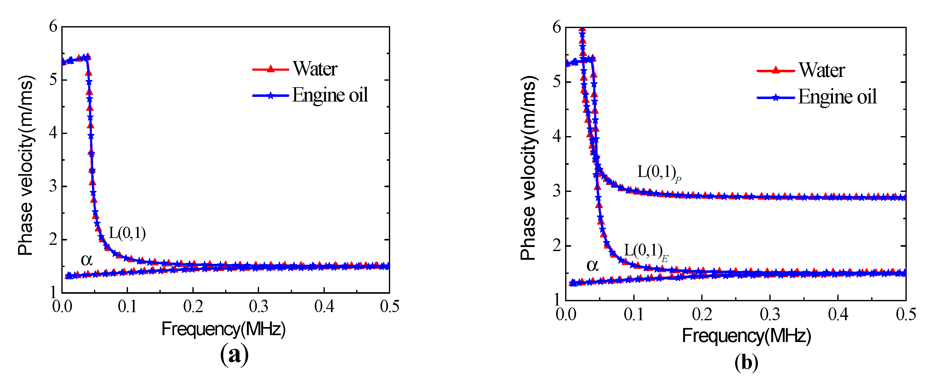
3.1.5. Influence of Pore Fluid

In this subsection, the pore fluid is changed from water to oil. The engine oil studied by Duan et al. [8] is analyzed here, such that longitudinal velocity $c_O=1740$ m/s and density ${\rho }_O=870$ kg/m³. The pipe is filled with water (see properties in the previous section) and the internal and external of pipe radii are a = 14 mm and b = 16 mm. Note that the values of $\beta$ = 0.1 and d = 0.05 m are used for the infinite and finite media in this subsection. The influence of pore fluid on the dispersion curves is shown in Figure 6.

It can be seen in Figure 6 that when engine oil is present, the phase velocity of each mode does not change significantly. The dispersion curves of the liquid-filled pipe when the pore fluid is engine oil are almost the same as when the pore fluid is water. Therefore, the propagation of the guided wave in the liquid-filled pipe embedded in porous medium is mainly determined by the external medium and the pipe. The fluid viscosity is not considered, given its small influence.

3.2. Results for Time Domain

Transient responses are here intuitively introduced to the observed dispersion characteristics of guided waves in the liquid-filled pipe system. Although the excitation source has a certain effect on the time-domain waveform, the inherent characteristics of the waveform are independent of the source. We use the cosine envelope pulse function as the excitation source, as the pulsed sound source represents a non-directional and isotropic monopole point sound [45]. In this study, we assume an acoustic point-source at the origin of the coordinates, and the point-source function is

$$x_0(t)=\{\begin{array}{l}\frac{1}{2}\left[1+\cos \frac{2\pi }{T_c}(t-\frac{T_c}{2})\right]\cos 2\pi f_0(t-\frac{T_c}{2}),(0\le t\le T_c)\\ 0,(t\le 0,t\ge T_c)\end{array}$$

(36)

Its transform is given by

$$X\left(f\right)=\frac{1}{4\pi }A\left(f\right)e^{\mathrm{j}\pi f{T}_c}$$

(37)

where T_c is the pulse length (T_c = 0.5 ms), and f0 is the frequency of the sound source (f₀ = 25 kHz). The Fourier–Bessel and Hankel transforms are frequently used as a tools for solving numerous scientific problems, and have become highly useful in the analysis of the wave field. The $u_{rE}$ and $u_{rPS}$ can be solved via (4) and (18). The two-dimensional Fourier transform of $u_r$ can generate the radial displacement time-domain curve.

The dispersion curves of guided waves in the liquid-filled pipe embedded in infinite and finite porous media are illustrated in Figure 2 and Figure 3, respectively. Figure 2 shows only two modes, α and L(0,1)_E, at the frequency 25 kHz. Figure 4 indicates three modes, α, L(0,1)_E and L(0,1)_P, when the frequency increases from 0.02 to 0.06 MHz. However, there are more than three different modes at any frequency when the frequency increases from 0.06 to 0.5 MHz, and the character of each mode is unique. To provide an illustrative example, we consider the pipe to be infinite, and analyze the time-domain waveform with regard to the signal acquisition, porosity, and thickness of the finite porosity medium layer. In this subsection, the acquisition locations are at the liquid–pipe interface in the infinite porous medium and at the external interface of the finite porous medium layer, which are 3 m away from the excitation source.

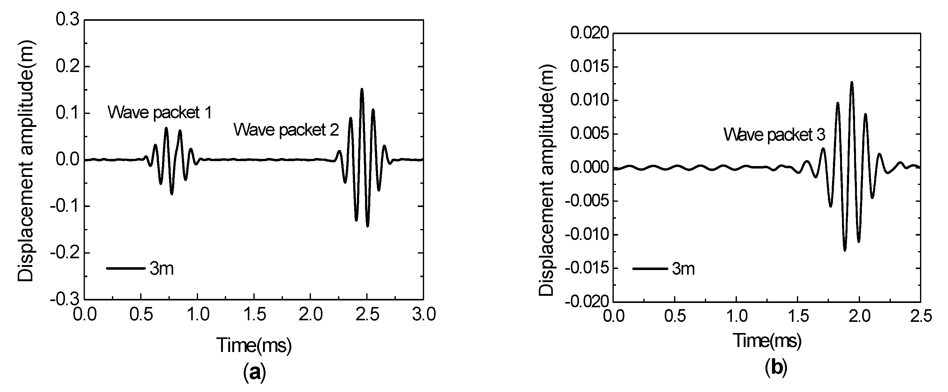
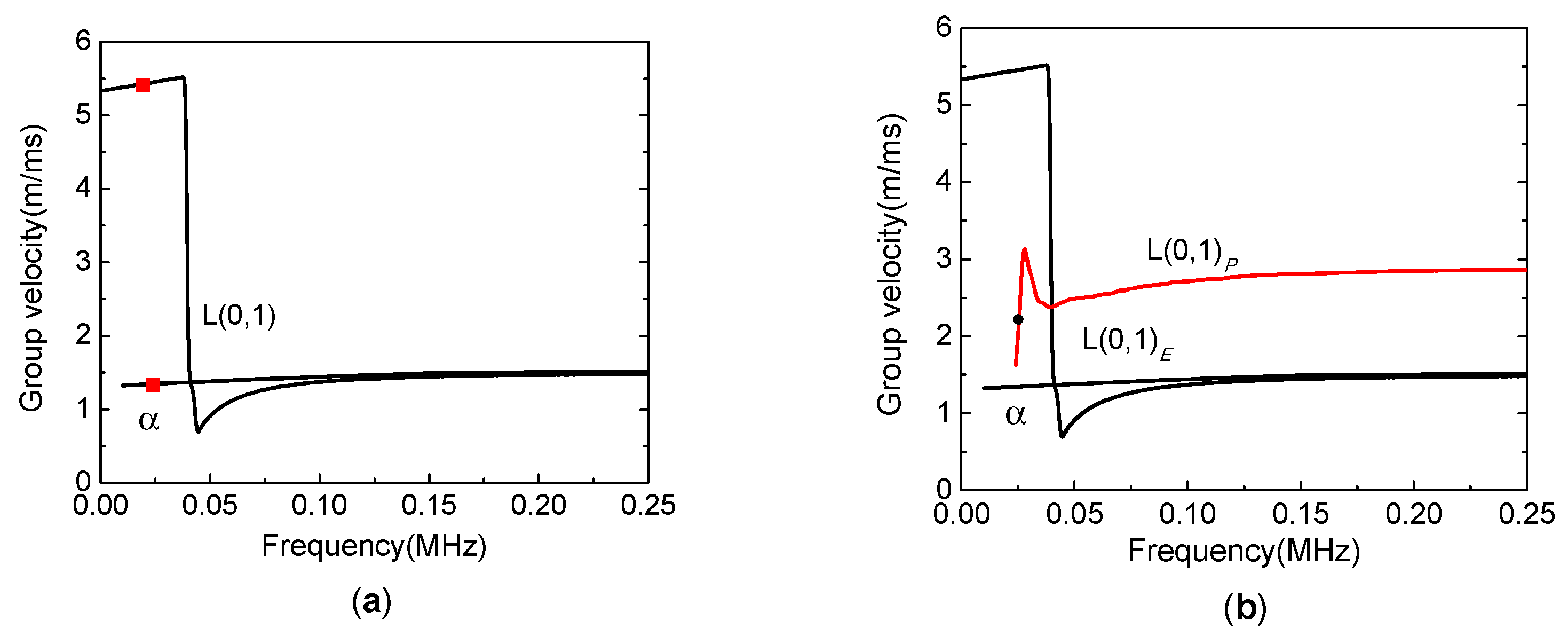
3.2.1. Discrimination of Guided Wave Modes

The time-domain waveforms at different acquisition interfaces with a porosity of 0.1 and a finite porosity medium layer thickness of 0.05 m are presented in Figure 7. In Figure 7a, the time-domain waveform of the liquid–pipe interface in the infinite porous medium consists of two unknown wave-packets, tagged wave-packet 1 and wave-packet 2, respectively. From Figure 7b, a similar observation is made for the case of the external interface of a finite porous medium. There is a wave-packet here, tagged wave-packet 3. Therefore, the conclusion that wave-packet 1, wave-packet 2, and wave-packet 3 at 25 kHz belong to mode L(0,1), α and L(0,1)_P, respectively, is deduced.

To verify the above conclusions, further numerical calculations are performed. For the liquid-filled pipe embedded in an infinite porous medium, the group velocity of wave-packet 1 is 5454 m/s, and the group velocity of the wave-packet 2 is 1333 m/s. These two velocities agree with the group velocity of modes L(0,1), α at 25 kHz, which is highlighted by square marks in Figure 8a, such that the wave-packets 1 and 2 are confirmed as the modes L(0,1) and α, respectively. Similarly, the velocity of wave-packet 3 with the arrival time and propagation distance is 1973 m/s at the external interface of the finite porous medium. This value is close to the velocity of mode L(0,1)_P at 25 kHz, as highlighted by the circular mark in Figure 8b. Thus, it can be concluded that wave-packet 3 is in the mode L(0,1)_P at the external interface of the finite porous medium. The inversion results show that only the α, L(0,1), and L(0,1)_P modes are found at two acquisition locations at a frequency of 25 kHz, and they have an excellent match with the dispersion curves in Figure 2 and Figure 3.

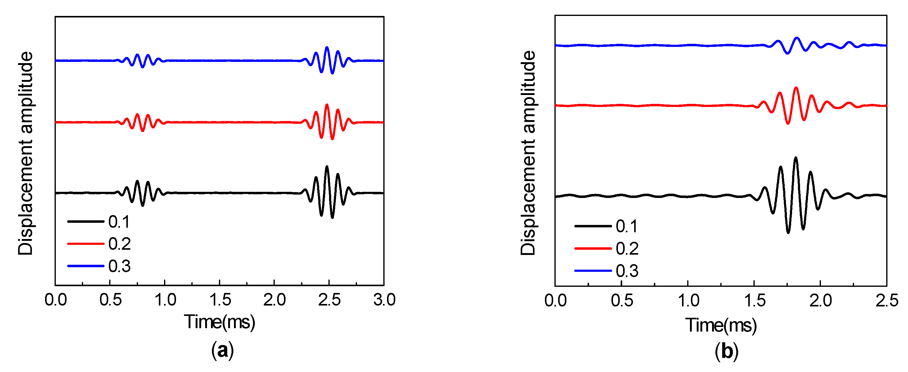
3.2.2. Influence of Porosity

As discussed in the previous subsection, the effect of porosity on the L(0,1)_P mode is strong enough to estimate the porosity of the medium surrounding the liquid-filled pipe. Subsequently, we convert the guided waves in the dispersion into the time-domain waveform to interpret the effect of porosity on the guided wave in the liquid-filled pipe embedded in a porous medium.

The effect of the change of porosity on the time-domain waveform with respect to time in the liquid-filled pipe embedded in infinite and finite porous media is depicted in Figure 9, when the porosity is varied between 0.1, 0.2, and 0.3. Figure 9a shows that as the porosity changes, the positional movement of two waves is not evident, and the dispersion characteristic indicates that there is no large change in the phase velocity, which is consistent with the conclusion obtained from Figure 2. At the external interface of the finite porous medium (Figure 9b), the waveform of the L(0,1)_P mode moves slightly backward with the increase in the porosity of the porous medium, which is due to the fact that the wave velocity decreases with porosity, as seen in Figure 4b. This also shows that the displacement amplitude of the wave is gradually reduced as the porosity increases.

3.2.3. Influence of Finite Porosity Layer Thickness

Considering that the structure of the pipe in the model is an important factor affecting the propagation characteristics of the waveform, this study uses a liquid-filled pipe embedded in a finite porous medium model, and analyzes the influence of the thickness of the finite porosity layer on the time-domain waveforms.

The time-domain waveforms in the liquid-filled pipe embedded in a finite porous medium with the same porosity value of $\beta$ = 0.1 and variable finite porosity layer thickness values of d = 0.025, 0.05, and 0.10 m are shown in Figure 10. The time-domain waveforms at the external interface of the finite porous medium are described, showing that the arrival time of the wave is almost independent of the thickness of the medium, and the displacement amplitude of the wave decreases with thickness [46].

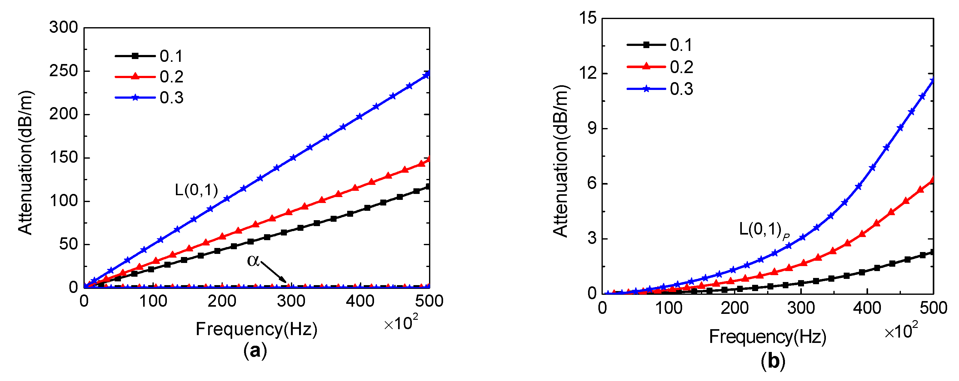
3.3. Results for Attenuation

Porous medium is dissipative in nature, and thus, the wave number k is complex. The waves generated obey a diffusion type process and therefore become attenuated. The imaginary part of the wave number corresponds to attenuation of waves [47]. A preliminary study of the effect of porosity on the dispersion characteristics and time-domain waveform was conducted by investigating the behavior of a liquid-filled pipe embedded in porous medium. There is a certain relationship between porosity and pipeline leakage. The results of this study are therefore presented to illustrate the nature of the attenuation, rather than as a rigorous validation. Nevertheless, fairly good agreement between the prediction and simulation was achieved.

Attenuation as a function of frequency is depicted in Figure 11 for a water-filled pipe embedded in porous medium with different values of porosity, i.e., $\beta$ = 0.1, 0.2, and 0.3. In Figure 11, we plot the attenuation curves of the α and L(0,1) modes. Figure 11a shows that the attenuation of α mode is zero; however, its mode shape is not suited to detection. At low frequencies, its axial displacement is dominant, but the actual set-up is not appropriate for imposing a displacement in the outer medium. At higher frequencies, its axial and radial displacements decrease exponentially from the outer wall, and again, the detection is not suitable to generate this mode. Aristégui and Lowe, in their study of fluid-filled pipes surrounded by different fluids [12], similarly found and discussed that the attenuation curve is zero. The attenuation of L(0,1) increases for higher values of frequency, first rapidly then almost linearly with frequency. The attenuation trends are practically identical for the different values of the porosity. Again, there is very good agreement between the dispersion characteristics and the attenuation. As investigated by Gao et al. [48], for a fluid-filled pipe surrounded by a fluid medium, the attenuation increases as a result of the added radiation damping. As shown in Figure 11a, the radiation damping effect increases with porosity (the water in the porous medium increases with the porosity). At very low frequencies (below 200 Hz), this effect is relatively small, whereas it increases distinguishably at higher frequencies relative to the value at low porosity. A similar phenomenon is observed in the case of the water-filled pipe embedded in finite porous medium from Figure 11b. It can be seen that a finite medium reduces radiation damping to the pipe wall, causing smaller losses [49]. It is observed that the attenuation in the water-filled pipe embedded in a finite porous medium decreases significantly compared to that in an infinite medium, this value being 1.79 dB/m for a finite porous medium and 103.17 dB/m for an infinite porous medium at 0.045 MHz ($\beta$ = 0.1).

By comparing Figure 11a,b, it can be seen that the attenuation taking place in a water-filled pipe when it is embedded in a finite porous medium is significantly less than that in a water-filled pipe embedded in an infinite porous medium. In both the cases, attenuation increases with porosity and wave frequency. This indicates that, in practice, a pipeline leak can be indirectly reflected by the value of porosity.

4. Conclusions

The influence of porosity on the propagation of longitudinal guided waves in a liquid-filled pipe embedded in a finite porous medium was investigated. The filling-liquid was assumed to be water, which is simulated by a linearized Navier–Stokes equation. A porous medium was assumed as the medium outside the pipes and was simulated by the modified Biot theory. This study of the longitudinal guided wave of a water-filled pipe embedded in infinite and finite porous media has led to the following conclusions:

(1)

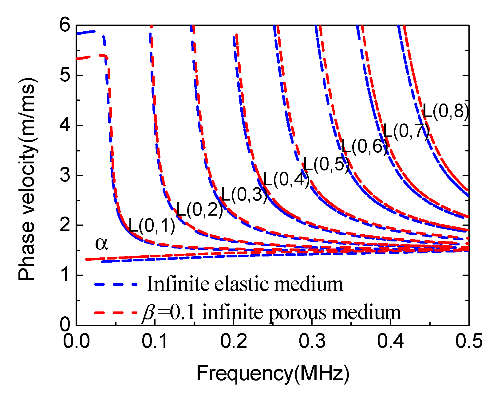
The presence of a porous medium outside the pipe has no significant effect on the phase velocity of a water-filled pipe, compared with a water-filled pipe embedded in an infinite elastic medium;

(2)

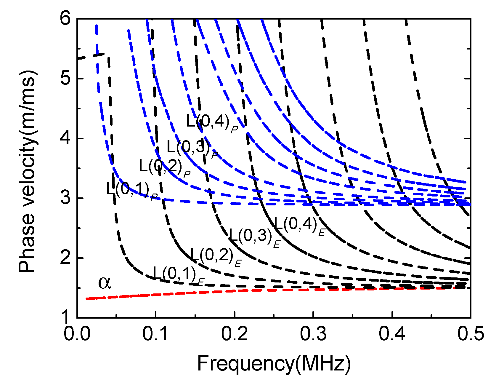
The number of modes in a water-filled pipe embedded in a finite porous medium is more than that of a water-filled pipe embedded in an infinite porous medium in the dispersion curves;

(3)

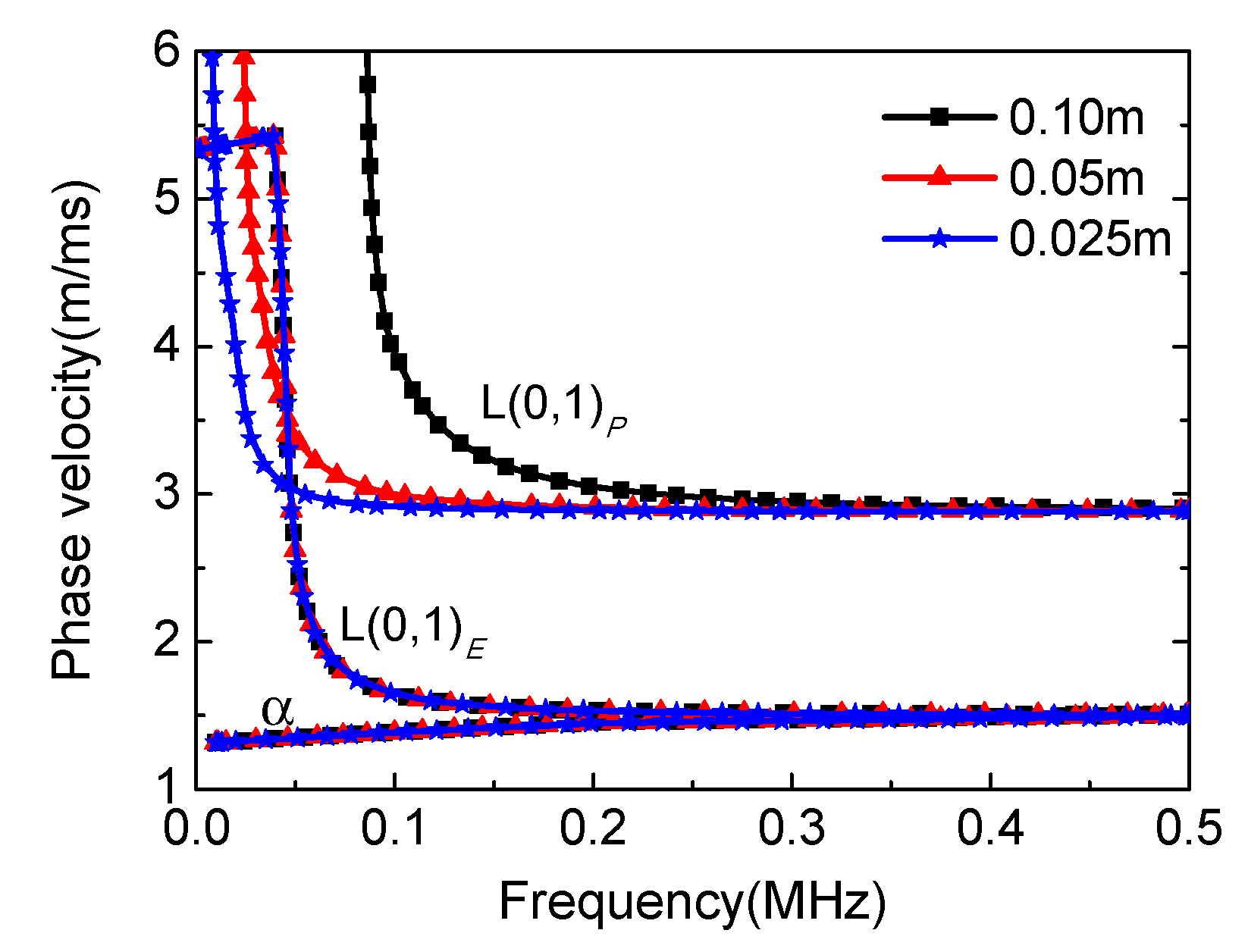
The effect of the finite medium surrounding the liquid-filled pipe has been shown by the appearance of several modes (L(0,m)_P, m = 1,2,3,…), and by the dependence of the phase velocity and displacement amplitude on an outer medium. A good agreement is thus obtained between the dispersion results, time-domain waveform, and attenuation;

(4)

The attenuation in a water-filled pipe when it is embedded in a finite porous medium is significantly less than that in a water-filled pipe embedded in an infinite porous medium;

(5)

The low attenuation L(0,1)_P mode is easily excited and detected, and it is strongly influenced by porosity. As the porosity increases, the phase velocity and displacement amplitude gradually decrease. This explains why, in practice, the pore content in the medium outside the liquid-filled pipe can indirectly indicate a pipeline leak, and provide a certain theoretical support for nondestructive testing.

With the model of a liquid-filled pipe embedded in infinite and finite porous media established in this paper, the porosity leads to a new aspect of optimization theory for pipeline leak detection, but the sound propagation characteristics still require refinement. In addition, future efforts will be directed toward the following aspects: (1) experimentation with the theoretical model to achieve mutual verification of theory and practice; (2) simulation of complicated pipe systems; and (3) investigation of other parameters, such as the pressure and viscosity coefficient.

5. Patents

The study in this manuscript resulted in a patent entitled “A Method for Leakage Detection of Buried Liquid-filled Pipes Based on Porous Media Parameters”, patent number ZL 2019 1 0084926.6.

References

1. Gazis, D.C. Three-dimensional investigation of the propagation of waves in hollow circular cylinders. I. Analytical foundation. J. Acoust. Soc. Am. 1959, 31, 573–578. [Google Scholar] [CrossRef]
2. Pan, H.; Koyano, K.; Usui, Y. Experimental and numerical investigations of axisymmetric wave propagation in cylindrical pipe filled with fluid. J. Acoust. Soc. Am. 2003, 113, 3209–3214. [Google Scholar] [CrossRef] [PubMed]
3. Duan, R.; Yang, K.; Ma, Y.; Chapman, N.R. A simple expression for sound attenuation due to surface duct energy leakage in low-latitude oceans. J. Acoust. Soc. Am. 2016, 139, EL118. [Google Scholar] [CrossRef] [PubMed] [Green Version]
4. Muggleton, J.M.; Kalkowski, M.; Gao, Y.; Rustighi, E. A theoretical study of the fundamental torsional wave in buried pipes for pipeline condition assessment and monitoring. J. Sound Vib. 2016, 374, 155–171. [Google Scholar] [CrossRef]
5. Nnaemeka, C.N.; Okorosaye-Orubiteine, K. Corrosion pattern of pipeline steel in petroleum pipeline water in the presence of biomas derived extracts of brassica oleracea and citrus paradise mesocarp. Mater. Sci. Appl. 2018, 9, 126–141. [Google Scholar]
6. Duan, W.; Kirby, R. Guided wave propagation in buried and immersed fluid-filled pipes: Application of the semi analytic finite element method. Comput. Struct. 2019, 212, 236–247. [Google Scholar] [CrossRef]
7. Yu, W.; Li, X. Propagation Characteristics and Defect Sensitivity Analysis of Guided Wave from Single Excitation Source in Elbows. IEEE Access 2019, 7, 75542–75549. [Google Scholar]
8. Muggleton, J.M.; Brennan, M.J.; Pinnington, P.J. Wavenumber prediction of waves in buried pipes for water leak detection. J. Sound Vib. 2002, 249, 939–954. [Google Scholar] [CrossRef]
9. Gao, Y.; Sui, F.; Muggleton, J.M.; Yang, J. Simplified dispersion relationships for fluid-dominated axisymmetric wave motion in buried fluid-filled pipes. J. Sound Vib. 2016, 375, 386–402. [Google Scholar] [CrossRef]
10. Sinha Bikash, K. Axisymmetric wave propagation in fluid-loaded cylindrical shells. i: Theory. J. Acoust. Soc. Am. 2019, 92, 1132–1143. [Google Scholar] [CrossRef]
11. Lafleur, L.D.; Shields, F.D. Low-frequency propagation modes in a liquid-filled elastic tube waveguide. J. Acoust. Soc. Am. 1995, 97, 1435–1445. [Google Scholar] [CrossRef]
12. Aristégui, C.; Lowe, M.; Cawley, P. Guided waves in fluid-filled pipes surrounded by different fluids. Ultrasonics 1999, 39, 367–375. [Google Scholar] [CrossRef]
13. Long, R.; Lowe, M.; Cawley, P. Attenuation characteristics of the fundamental modes that propagate in buried iron water pipes. Ultrasonics 2003, 41, 509–519. [Google Scholar] [CrossRef]
14. Siqueira, M.H.S.; Gatts, C.E.N.; da Silva, R.R.; Rebello, J.M.A. The use of ultrasonic guided waves and wavelets analysis in pipe inspection. Ultrasonics 2004, 41, 785–797. [Google Scholar] [CrossRef]
15. Leinov, E.; Lowe, M.; Cawley, P. Investigation of guided wave propagation and attenuation in pipe buried in sand. J. Sound Vib. 2015, 347, 96–114. [Google Scholar] [CrossRef] [Green Version]
16. Cui, H.; Lin, W.; Zhang, H.; Wang, X.; Trevelyan, J. Backward waves with double zero-group-velocity points in a liquid-filled pipe. J. Acoust. Soc. Am. 2016, 139, 1179–1194. [Google Scholar] [CrossRef] [PubMed] [Green Version]
17. Long, R.; Cawley, P.; Lowe, M.J.S. Acoustic wave propagation in buried iron water pipes. Proc. Math. Phys. Eng. Sci. 2003, 459, 2749–2770. [Google Scholar] [CrossRef]
18. Ambrosini, R.D. Material damping vs. radiation damping in soil–structure interaction analysis. Comput. Geotech. 2006, 33, 86–92. [Google Scholar] [CrossRef]
19. Guan, W.; Hu, H.; He, X. Finite-difference modeling of the monopole acoustic logs in a horizontally stratified porous formation. J. Acoust. Soc. Am. 2009, 125, 1942–1950. [Google Scholar] [CrossRef]
20. Markov, A.M.; Markov, M.G.; Ronquillo, J.G.; Sadovnychiy, S.N. Acoustic reverberation in a logging tool-borehole-saturated porous medium system. Izv. Phys. Solid Eart. 2014, 50, 289–295. [Google Scholar] [CrossRef]
21. Zhou, F.; Giannakis, I.; Giannopoulos, A.; Holliger, K.; Slob, E. Estimating reservoir permeability with borehole radar. Geophysics 2020, 85, 1–42. [Google Scholar] [CrossRef]
22. Wang, W.; Zhu, X.; Liu, J.; Cui, Z. Shear-horizontal transverse-electric seismoelectric waves in cylindrical double layer porous media. Chin. Phys. B 2021, 30, 014301. [Google Scholar] [CrossRef]
23. Biot, M.A. Theory of propagation of elastic waves in a fluid-saturated porous solid. I. Low-frequency range. J. Acoust. Soc. Am. 1956, 28, 168–178. [Google Scholar] [CrossRef]
24. Biot, M.A. Theory of propagation of elastic waves in a fluid-saturated porous solid. II. Higher frequency range. J. Acoust. Soc. Am. 1956, 28, 179–191. [Google Scholar] [CrossRef]
25. Biot, M.A. Mechanics of deformation and acoustic propagation in porous media. J. Appl. Phys. 1962, 33, 1483–1498. [Google Scholar] [CrossRef]
26. Biot, M.A. Theory of viscous buckling of multilayered fluids undergoing finite strain. Phys. Fluids 1964, 7, 855–861. [Google Scholar] [CrossRef]
27. Johnson, D.L.; Koplik, J.; Dashen, R. Theory of dynamic permeability and tortuosity in fluid-saturated porous media. J. Fluid Mech. 1987, 176, 379–402. [Google Scholar] [CrossRef]
28. Mohr, W.; Holler, P. On inspection of thin-walled tubes for transverse and longitudinal flaws by guided ultrasonic waves. IEEE Trans. Sonics Ultrason. 1976, 23, 369–373. [Google Scholar] [CrossRef]
29. Cui, H.; Zhang, B.; Ji, S. Propagation characteristics of guided waves in a rod surrounded by an infinite solid medium. Acoust. Phys. 2010, 56, 412–421. [Google Scholar] [CrossRef]
30. Butt, H.S.U.; Xue, P.; Jiang, T.; Wang, B. Parametric identification for material of viscoelastic SHPB from wave propagation data incorporating geometrical effects. Int. J. Mech. Sci. 2015, 91, 46–54. [Google Scholar] [CrossRef]
31. Van Dalen, K.N.; Drijkoningen, G.G.; Smeulders, D.M.J. On wavemodes at the interfaxce of a fluid and a fluid-saturated poroelastic solid. J. Acoust. Soc. Am. 2010, 127, 40–51. [Google Scholar] [CrossRef]
32. Qingrui, L.; Katsube, N. The discovery of a second kind of rotational wave in a fluid-filled porous material. J. Acoust. Soc. Am. 1990, 88, 1045–1053. [Google Scholar]
33. Mavko, G.; Jizba, D. Estimating grain-scale fluid effects on velocity dispersion in rocks. Geophysics 1991, 56, 1940–1949. [Google Scholar] [CrossRef]
34. Xi, Z.; Yam, L.H.; Leung, T.P. Free vibration of a partially fluid-filled cross-ply laminated composite circular cylindrical shell. J. Acoust. Soc. Am. 1997, 28, 359–374. [Google Scholar] [CrossRef]
35. Chang, C.; Yuan, F. Extraction of Guided Wave Dispersion Curve in Isotropic and Anisotropic Materials by Matrix Pencil Method. Ultrasonics 2018, 89, 143–154. [Google Scholar] [CrossRef]
36. Parra, J.O.; Xu, P. Dispersion and attenuation of acoustic guided waves in layered fluid-filled porous media. J. Acoust. Soc. Am. 1994, 95, 91–98. [Google Scholar] [CrossRef]
37. Gravenkamp, H.; Birk, C.; Van, J. Modeling ultrasonic waves in elastic waveguides of arbitrary cross-section embedded in infinite solid medium. Comput. Struct. 2015, 149, 61–71. [Google Scholar] [CrossRef]
38. Su, N.; Han, Q.; Jiang, J. Guided circumferential wave propagation characteristics for porous cylinder immersed in infinite fluid. Acta Phys. Sin. 2019, 68, 152–160. [Google Scholar]
39. Abdelouahab, N.B.; Gossard, A.; Marlière, C.; Faure, P.; Rodts, S.; Coussot, P. Controlled imbibition in a porous medium from a soft wet material (poultice). Soft Matter 2019, 15, 6732–6741. [Google Scholar] [CrossRef]
40. Chang, S.; Liu, L.; Johnson, D.L. Low-frequency tube waves in permeable rocks. Geophysics 1988, 53, 519–527. [Google Scholar] [CrossRef]
41. Marston, P.L. Negative group velocity lamb waves on plates and applications to the scattering of sound by shells. J. Acoust. Soc. Am. 2003, 113, 2659–2662. [Google Scholar] [CrossRef] [PubMed]
42. Jiang, J.; Han, Q.; Xu, Z.; Jia, J.; Liang, D.; Zhong, X. Propagation characteristics of guided waves in a liquid filled pipe embedded in a porous medium. Acta Acust. 2020, 39, 96–109. [Google Scholar]
43. Lowe, M.J.S.; Cawley, P. The applicability of plate wave techniques for the inspection of adhesive and diffusion bonded joints. J. Nondestruct. Eval. 1994, 13, 185–200. [Google Scholar] [CrossRef]
44. Chotiros, N.P. Acoustics of the Seabed as a Poroelastic Medium; ASA: Austin, TX, USA, 2017. [Google Scholar]
45. Chernoyarov, O.V.; Lysina, E.A.; Marcokova, M.; Dachian, S. Statistical analysis of fast fluctuating random signals with arbitrary-function envelope under breach of consistency of discontinuous information parameter estimate. In Proceedings of the International Siberian Conference on Control and Communications (SIBCON), Omsk, Russia, 21–23 May 2015; pp. 1–11. [Google Scholar]
46. Haroun, N.A.H.; Mondal, S.; Sibanda, P. Hydromagnetic nanofluids flow through a porous medium with thermal radiation, chemical reaction and viscous dissipation using the spectral relaxation method. Int. J. Comput. Meth. 2017, 16, 1840020. [Google Scholar] [CrossRef]
47. Chinta, N.; Syed, A.S.; Modem, R.; Mangipudi, V.R. A Study on Propagation of Waves in a Transversely Isotropic Poroelastic Layer Bounded between Two Viscous Liquids. Open J. Acoust. 2019, 9, 1–12. [Google Scholar] [CrossRef] [Green Version]
48. Gao, Y.; Liu, Y.; Muggleton, J.M. Axisymmetric fluid-dominated wave in fluid-filled plastic pipes: Loading effects of surrounding elastic medium. Appl. Acoust. 2017, 116, 43–49. [Google Scholar] [CrossRef]
49. Barshinger, J.N.; Rose, J.L. Guided wave propagation in an elastic hollow cylinder coated with a viscoelastic material. IEEE Trans. Ultrason. Ferroelectr. Freq. Control 2004, 51, 1547–1556. [Google Scholar] [CrossRef] [PubMed]
Figure 1. Model geometry of a liquid-filled pipe embedded in porous medium.
Applsci 11 02281 g001
Figure 2. Dispersion curves of guided waves in water-filled pipe embedded in different media. The internal and external radii of the pipe are a = 14 mm and b = 16 mm, respectively. The vertical and horizontal axes depict the phase velocity and frequency. Blue and red lines represent propagating modes in the water-filled pipe embedded in infinite elastic and porous media, respectively.
Applsci 11 02281 g002
Figure 3. Dispersion curves of guided waves in water-filled pipe embedded in finite porous medium of porosity 0.1. The thickness of the finite porous medium is d = 0.05 m. Red, black, and blue lines represent three kinds of modes: α mode, L(0,m)E, and L(0,m)P(m = 1,2,3,…,8), respectively.
Applsci 11 02281 g003
Figure 4. Dispersion curves of guided waves in a water-filled pipe embedded in (a) infinite porous medium and (b) finite porous medium. The thickness of the finite porous medium is d = 0.05 m. Black, red, and blue lines represent the porosity β = 0.1, 0.2, and 0.3, respectively.
Applsci 11 02281 g004
Figure 5. Dispersion curves of guided waves in water-filled pipe embedded in a finite porous medium of layer thickness d = 0.025, 0.05, 0.10 m. Porosity is β = 0.1. Black, red, and blue lines represent layer thicknesses d = 0.025, 0.05, and 0.10 m, respectively.
Applsci 11 02281 g005
Figure 6. Dispersion curves of guided waves in water-filled pipe embedded in (a) infinite porous medium, and (b) finite porous medium. The thickness of the finite porous medium is d = 0.05 m. Porosity is β = 0.1. Red and blue lines represent the different pore fluids of water and engine oil, respectively.
Applsci 11 02281 g006
Figure 7. Time-domain waveform of radial displacement with respect to time ( β = 0.1) (a) at the liquid–pipe interface in infinite porous medium and (b) at the external interface of the finite porous medium. The thickness of the finite porous medium is d = 0.05 m. The vertical and horizontal axes depict the displacement amplitude and time.
Applsci 11 02281 g007
Figure 8. Group velocity dispersion curves of the first three orders of modes in the water-filled pipe embedded in ( β = 0.1) (a) infinite porous medium and (b) finite porous medium.
Applsci 11 02281 g008
Figure 9. Time-domain waveforms with respect to time for various values of porosity in an infinite porous medium (a) at the liquid–pipe interface and (b) at the external interface of the finite porous medium. The thickness of finite porous medium is d = 0.05 m. Black, red, and blue lines represent the porosity values of β = 0.1, 0.2, and 0.3, respectively.
Applsci 11 02281 g009
Figure 10. Time-domain waveforms with respect to time for various thicknesses of porous medium layer ( β = 0.1). Black, red and blue lines represent layer thickness d = 0.025, 0.05, and 0.10 m, respectively.
Applsci 11 02281 g010
Figure 11. Attenuation curves of guided waves in water-filled pipe embedded in (a) infinite porous medium and (b) finite porous medium. The thickness of finite porous medium is d = 0.05 m. Black, red, and blue lines represent the porosity values of β = 0.1, 0.2, and 0.3, respectively.
Applsci 11 02281 g011