Estimating the Entropy of Binary Time Series: Methodology, Some Theory and a Simulation Study

Abstract
:1. Introduction
- Due its computational inefficiency, the plug-in estimator is the least reliable method, in contrast to the LZ-based estimators and the CTW, which naturally incorporate dependencies in the data at much larger time scales.
- The most effective estimator is the CTW method. Moreover, for the CTW as well as for all other estimators, the main source of error is the bias and not the variance.
- Among the four LZ-based estimators, the two most efficient ones are those with increasing win- dow sizes, Ĥn of [9] and introduced in Section 2.3. Somewhat surprisingly, in several of the simulations we conducted the performance of the LZ-based estimators appears to be very similar to that of the plug-in method.
2. Entropy Estimators and Their Properties
2.1. Entropy and Entropy Rate

2.2. The Plug-in Estimator
2.3. The Lempel-Ziv Estimators


- (i)
- When applied to an arbitrary data string, the estimators defined in (3)–(6) always satisfy,for any n, k.
- (ii)
- The estimators Ĥn,k and Ĥn are consistent when applied to data generated by a finite-valued, stationary, ergodic process that satisfies Doeblin’s condition (DC). With probability one we have:Ĥn,k → H, Ĥn → H, as k, n → ∞.
- (iii)
- The estimators and are consistent when applied to data generated by an arbitrary finite-valued, stationary, ergodic process, even if (DC) does not hold. With probability one we have:
- If the two limits as n and k tend to infinity are taken separately, i.e., first k → ∞ and then n → ∞, or vice versa;
- If k → ∞ and n = nk varies with k in such a way that nk → ∞ as k → ∞;
- If n → ∞ and k = kn varies with n in such a way that it increases to infinity as n → ∞;
- If k and n both vary arbitrarily in such a way that k stays bounded and n → ∞.


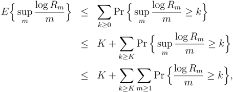

2.4. Bias and Variance of the LZ-based Estimators
2.5. Context-Tree Weighting


3. Results on Simulated Data
3.1 Statistical Models and Their Entropy Rates
3.1.1 I.I.D. (or “homogeneous Poisson”) Data
3.1.2. Markov Chains
3.1.3 Hidden Markov Models

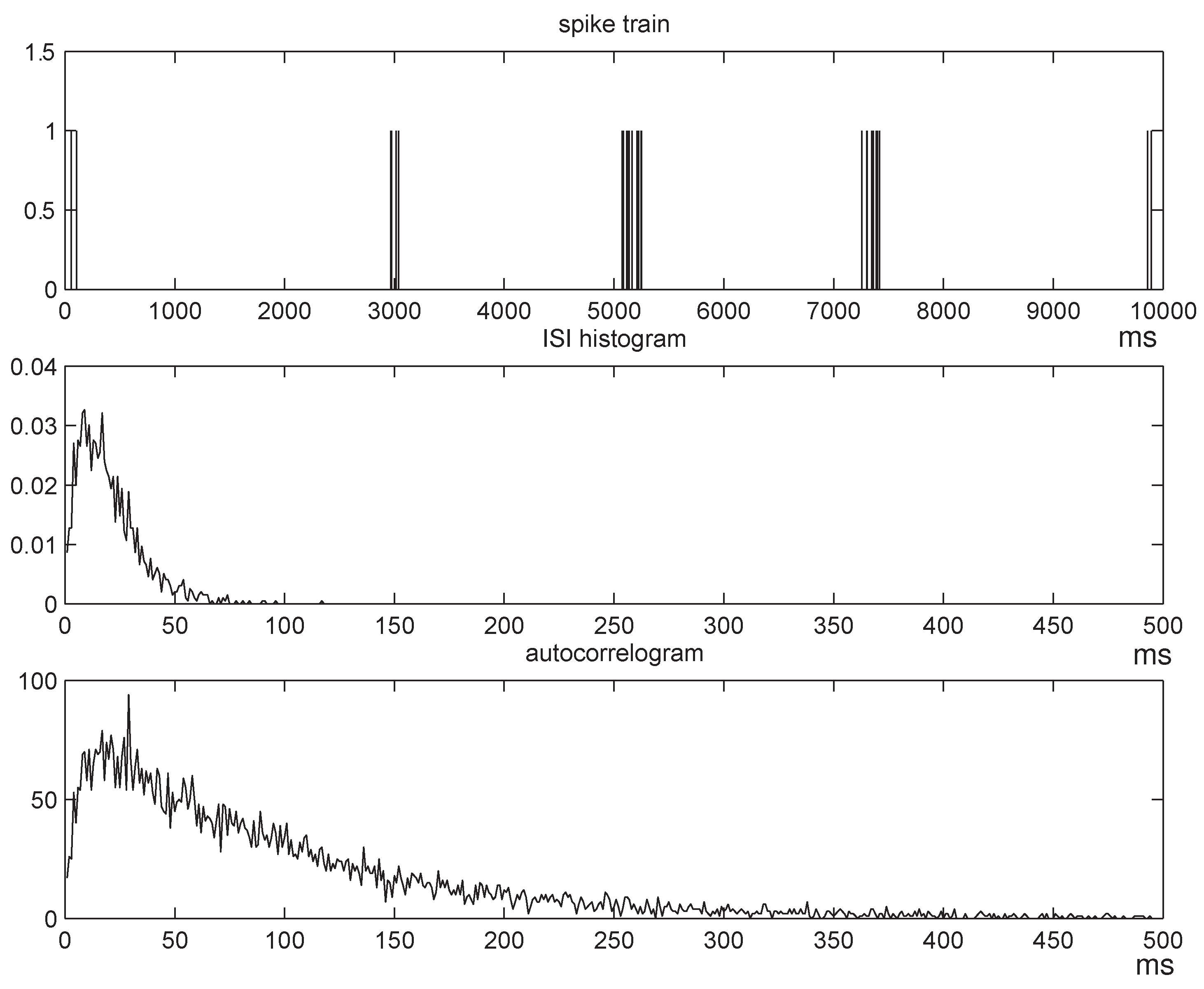
3.1.4. Renewal Processes
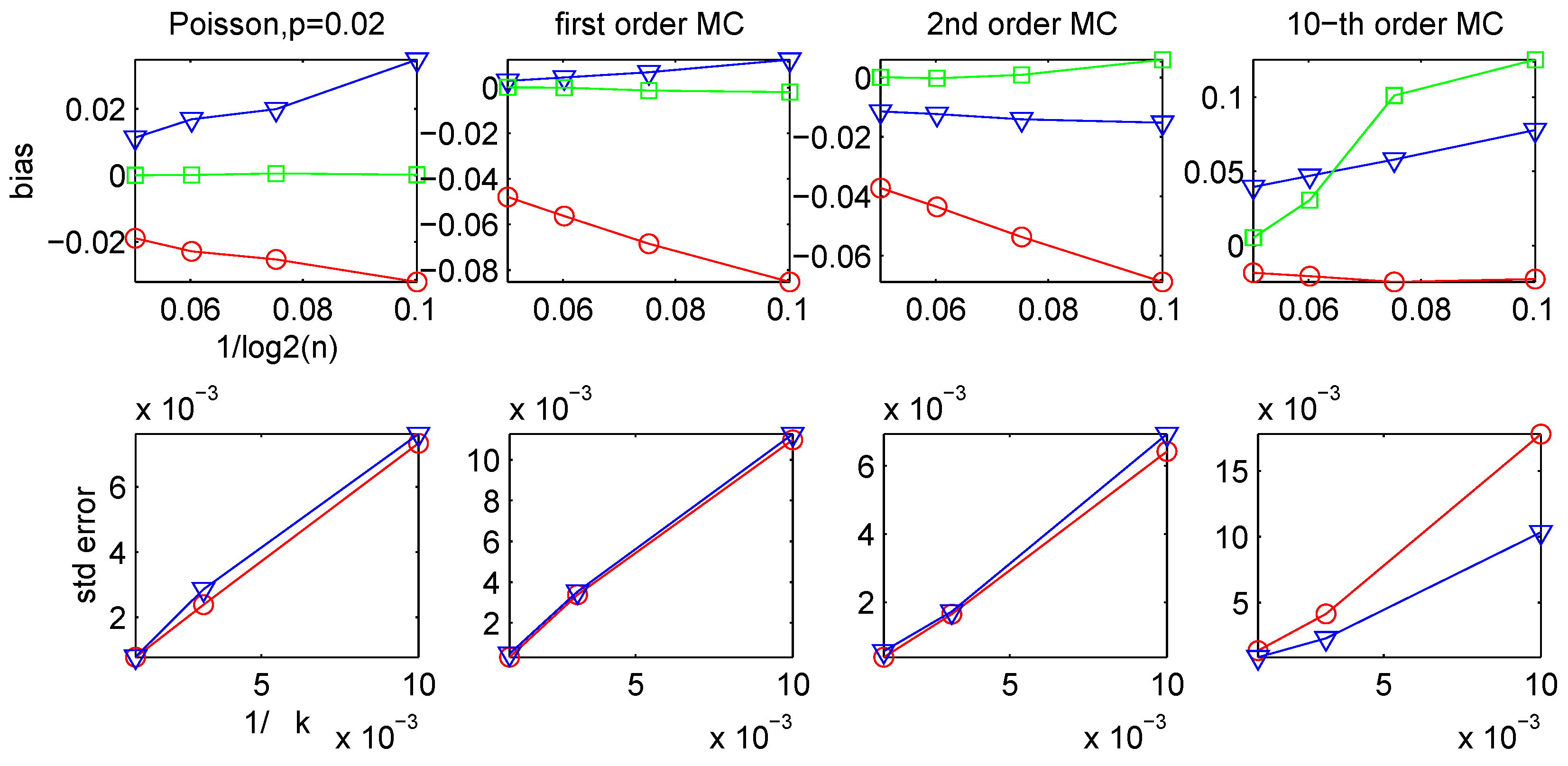
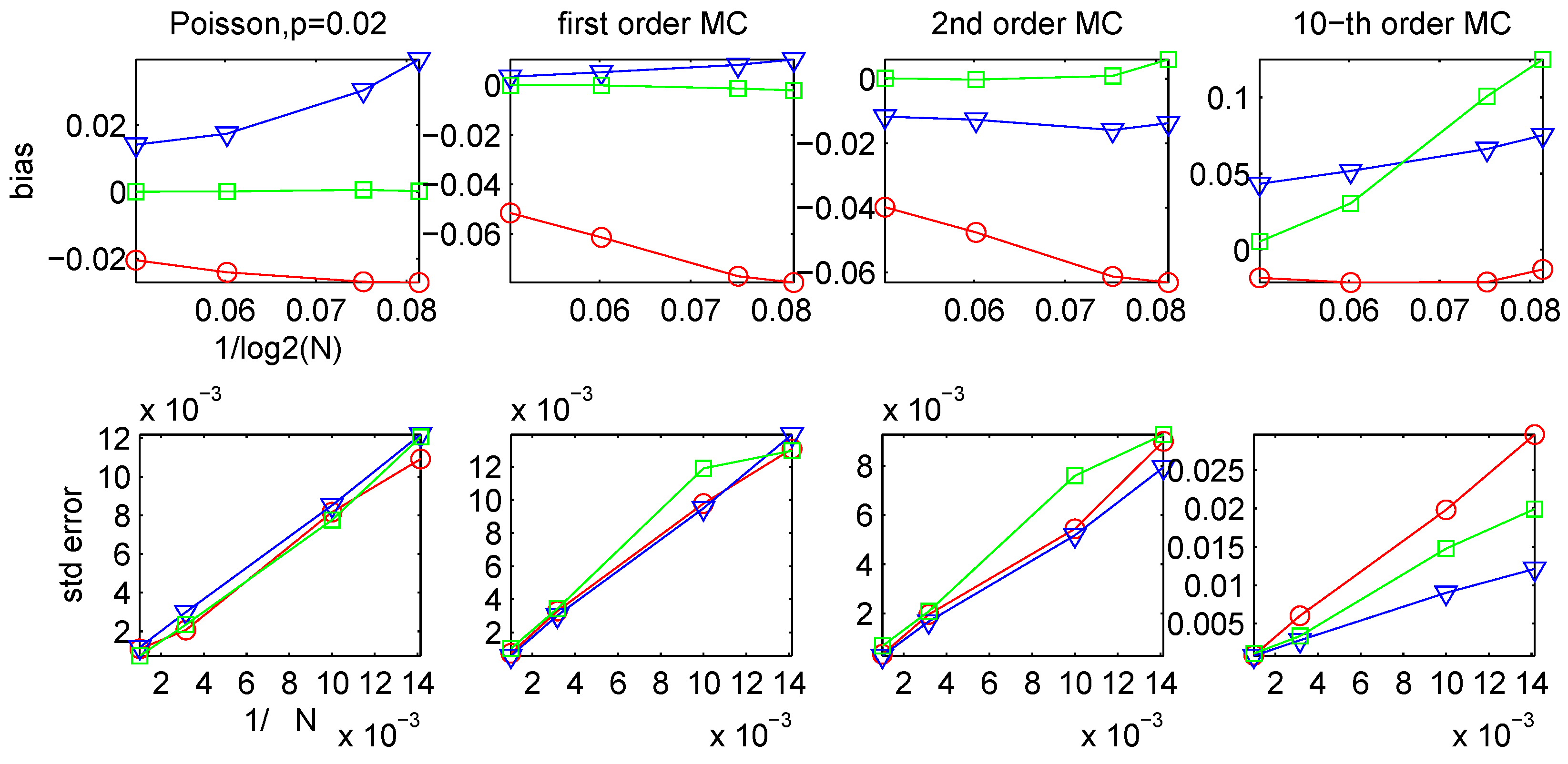
3.2. Bias and Variance of the CTW and the LZ-based Estimators


| Ĥn,k | ||||||||
| n/k | n | k | bias | std err | MSE | bias | std err | MSE |
| 1 | 499980 | 499980 | -0.0604 | 0.0010 | 0.1824 | -0.0325 | 0.0009 | 0.0528 |
| 10 | 909054 | 90906 | -0.0584 | 0.0018 | 0.1705 | -0.0318 | 0.0019 | 0.0507 |
| 100 | 990059 | 9901 | -0.0578 | 0.0066 | 0.1692 | -0.0315 | 0.0067 | 0.0517 |
| 1000 | 998961 | 999 | -0.0553 | 0.0200 | 0.1732 | -0.0297 | 0.0210 | 0.0663 |
| 10000 | 999860 | 100 | -0.0563 | 0.0570 | 0.3209 | -0.0356 | 0.0574 | 0.2280 |
| Ĥn,k | ||||
| k = 105 | k = 106 | |||
| case | bootstrap | std dev | bootstrap | std dev |
| 1 | 0.0018 | 0.0025 | 0.0006 | 0.0009 |
| 2 | 0.0025 | 0.0023 | 0.0008 | 0.0009 |
| 3 | 0.0015 | 0.0019 | 0.0005 | 0.0007 |
| 4 | 0.0061 | 0.0073 | 0.0017 | 0.0023 |
| k = 105 | k = 106 | |||
| case | bootstrap | std dev | bootstrap | std dev |
| 1 | 0.0033 | 0.0033 | 0.0011 | 0.0010 |
| 2 | 0.0031 | 0.0025 | 0.0010 | 0.0009 |
| 3 | 0.0017 | 0.0016 | 0.0006 | 0.0006 |
| 4 | 0.0032 | 0.0031 | 0.0009 | 0.0010 |

3.3. Comparison of the Different Entropy Estimators
| Data model | plug-in w = 15 | plug-in w = 20 | Ĥn | CTW | ||
| i.i.d. | % of bias | 0.001 | -0.10 | -14.47 | 9.98 | 0.04 |
| % of stderr | 0.57 | 0.51 | 0.77 | 0.83 | 0.51 | |
| % of | 0.57 | 0.52 | 14.49 | 10.01 | 0.52 | |
| 1st order MC | % of bias | -0.11 | -0.78 | -10.38 | 0.70 | 0.02 |
| % of stderr | 0.22 | 0.16 | 0.15 | 0.12 | 0.21 | |
| % of | 0.25 | 0.80 | 10.38 | 0.71 | 0.21 | |
| 2nd order MC | % of bias | 4.16 | 1.72 | -5.32 | -1.56 | 0.02 |
| % of stderr | 0.08 | 0.08 | 0.04 | 0.04 | 0.09 | |
| % of | 4.16 | 1.73 | 5.32 | 1.56 | 0.09 | |
| 10th order MC | % of bias | 16.04 | 10.03 | -2.66 | 6.23 | 0.77 |
| % of stderr | 0.19 | 0.14 | 0.13 | 0.12 | 0.16 | |
| % of | 16.04 | 10.04 | 2.66 | 6.24 | 0.78 |
| HMM | plug-in w = 15 | plug-in w = 20 | Ĥn | CTW | ||
| 3 states | % of bias | 4.05 | 3.69 | -43.41 | 11.46 | 2.51 |
| % of stderr | 2.43 | 2.43 | 1.79 | 2.64 | 2.41 | |
| % of | 4.74 | 4.43 | 43.47 | 11.75 | 3.50 | |
| 50 states | % of bias | 2.98 | 2.53 | -35.62 | 5.39 | 2.31 |
| % of stderr | 3.26 | 3.25 | 3.15 | 3.35 | 3.26 | |
| % of | 4.43 | 4.12 | 35.76 | 6.33 | 4.00 |

| (α2, β2) | renewal entropy | plug-in w = 20 | Ĥn | CTW | ||
| (10,20) | % of bias | -0.06 | 6.09 | -20.98 | 21.84 | 1.66 |
| % of stderr | 0.73 | 0.77 | 0.66 | 0.95 | 0.72 | |
| % of | 0.74 | 6.14 | 20.99 | 21.86 | 1.81 | |
| (50,20) | % of bias | -1.53 | 25.90 | -30.38 | 81.40 | 7.64 |
| % of stderr | 2.37 | 3.03 | 0.79 | 2.67 | 2.38 | |
| % of | 2.82 | 26.08 | 30.39 | 81.45 | 8.00 | |
| (50,50) | % of bias | -5.32 | 34.35 | -50.64 | 85.61 | 3.58 |
| % of stderr | 2.36 | 3.12 | 0.69 | 2.67 | 2.42 | |
| % of | 5.82 | 34.49 | 50.65 | 85.65 | 4.32 |
4. Summary and Concluding Remarks
- (i)
- For all estimators considered, the main source of error is the bias.
- (ii)
- Among all the different estimators, the CTW method is the most effective; it was repeatedly and consistently seen to provide the most accurate and reliable results.
- (iii)
- No significant benefit is derived from using the finite-context-depth version of the CTW.
- (iv)
- Among the four LZ-based estimators, the two most efficient ones are those with increasing window sizes, Ĥn, . No systematic trend was observed regarding which one of the two is more accurate.
- (v)
- Interestingly (and somewhat surprisingly), in many of our experiments the performance of the LZ-based estimators was quite similar to that of the plug-in method.
- (vi)
- The main drawback of the plug-in method is its computational inefficiency; with small word-lengths it fails to detect longer-range structure in the data, and with longer word-lengths the empirical distribution is severely undersampled, leading to large biases.
- (vii)
- The renewal entropy estimator, which is only consistent for data generated by a renewal process, suffers a drawback similar (although perhaps less severe) to the plug-in.
Acknowledgements
References
- Miller, G. Note on the bias of information estimates. In Information theory in psychology; Quastler, H., Ed.; Free Press: Glencoe, IL, 1955; pp. 95–100. [Google Scholar]
- Basharin, G. On a statistical estimate for the entropy of a sequence of independent random variables. Theor. Probability Appl. 1959, 4, 333–336. [Google Scholar] [CrossRef]
- Grassberger, P. Estimating the information content of symbol sequences and efficient codes. IEEE Trans. Inform. Theory 1989, 35, 669–675. [Google Scholar] [CrossRef]
- Shields, P. Entropy and prefixes. Ann. Probab. 1992, 20, 403–409. [Google Scholar] [CrossRef]
- Kontoyiannis, I.; Suhov, Y. Prefixes and the entropy rate for long-range sources Chapter. In Proba-bility Statistics and Optimization; Kelly, F.P., Ed.; Wiley: New York, 1994. [Google Scholar]
- Treves, A.; Panzeri, S. The upward bias in measures of information derived from limited data samples. Neural Comput. 1995, 7, 399–407. [Google Scholar] [CrossRef]
- Schu¨rmann, T.; Grassberger, P. Entropy estimation of symbol sequences. Chaos 1996, 6, 414–427. [Google Scholar]
- Kontoyiannis, I. The complexity and entropy of literary styles, NSF Technical Report no. 97. 1996. [Available from pages.cs.aueb.gr/users/yiannisk/].
- Kontoyiannis, I.; Algoet, P.; Suhov, Y.; Wyner, A. Nonparametric entropy estimation for stationary processes and random fields, with applications to English text. IEEE Trans. Inform. Theory 1998, 44, 1319–1327. [Google Scholar] [CrossRef]
- Darbellay, G.; Vajda, I. Estimation of the information by an adaptive partitioning of the observation space. IEEE Trans. Inform. Theory 1999, 45, 1315–1321. [Google Scholar] [CrossRef]
- Victor, J. Asymptotic Bias in Information Estimates and the Exponential (Bell) Polynomials. Neural Comput. 2000, 12, 2797–2804. [Google Scholar] [CrossRef]
- Antos, A.; Kontoyiannis, I. Convergence properties of functional estimates for discrete distributions. Random Structures & Algorithms 2001, 19, 163–193. [Google Scholar]
- Paninski, L. Estimation of entropy and mutual information. Neural Comput. 2003, 15, 1191–1253. [Google Scholar] [CrossRef]
- Cai, H.; Kulkarni, S.; Verdú, S. Universal entropy estimation via block sorting. IEEE Trans. Inform. Theory 2004, 50, 1551–1561, Erratum, ibid., vol. 50, no. 9, p. 2204. [Google Scholar] [CrossRef]
- Brown, P.; Della Pietra, S.; Della Pietra, V.; Lai, J.; Mercer, R. An estimate of an upper bound for the Entropy of English. Computational Linguistics 1992, 18, 31–40. [Google Scholar]
- Chen, S.; Reif, J. Using difficulty of prediction to decrease computation: Fast sort, priority queue and convex hull on entropy bounded inputs. In 34th Symposium on Foundations of Computer Science, Los Alamitos, California, 1993; pp. 104–112.
- M. F.; et al. On the entropy of DNA: Algorithms and measurements based on memory and rapid convergence. In Proceedings of the 1995 Sympos. on Discrete Algorithms, 1995.
- Stevens, C.; Zador, A. Information through a Spiking Neuron. NIPS, 1995; 75–81. [Google Scholar]
- Teahan, W.; Cleary, J. The entropy of English using PPM-based models. In Proc. Data Compression Conf. – DCC 96, Los Alamitos, California, 1996; pp. 53–62.
- Strong, S. P.; Koberle, R.; de Ruyter van Steveninck, R.; Bialek, W. Entropy and Information in Neural Spike Trains. Phys. Rev. Lett. 1998, 80, 197–200. [Google Scholar] [CrossRef]
- Suzuki, R.; Buck, J.; Tyack, P. Information entropy of humpback whale song. The Journal of the Acoustical Society of America 1999, 105, 1048–1048. [Google Scholar] [CrossRef]
- Loewenstern, D.; Yianilos, P. Significantly Lower Entropy Estimates for Natural DNA Sequences. Journal of Computational Biology 1999, 6, 125–142. [Google Scholar] [CrossRef] [PubMed]
- Levene, M.; Loizou, G. Computing the entropy of user navigation in the web. International Journal of Information Technology and Decision Making 2000, 2, 459–476. [Google Scholar] [CrossRef]
- Reinagel, P. Information theory in the brain. Current Biology 2000, 10, 542–544. [Google Scholar] [CrossRef]
- London, M. The information efficacy of a synapse. Nature Neurosci. 2002, 5, 332–340. [Google Scholar] [CrossRef] [PubMed]
- Bhumbra, G.; Dyball, R. Measuring spike coding in the rat supraoptic nucleus. The Journal of Physiology 2004, 555, 281–296. [Google Scholar] [CrossRef] [PubMed]
- Nemenman, W.; Bialek, W.; de Ruyter van Steveninck, R. Entropy and information in neural spike trains: Progress on the sampling problem. Physical Review E 2004, 056111. [Google Scholar] [CrossRef] [PubMed]
- Warland, D.; Reinagel, P.; Meister, M. Decoding visual infomation from a population of retinal ganglion cells. J. of Neurophysiology 1997, 78, 2336–2350. [Google Scholar]
- Kennel, M.; Mees, A. Context-tree modeling of observed symbolic dynamics. Physical Review E 2002, 66. [Google Scholar] [CrossRef] [PubMed]
- Amigo’, J.M.; Szczepan’ski, J.M.; Wajnryb, E.M.; Sanchez-vives, M.V. Estimating the entropy rate of spike trains via Lempel-Ziv complexity. Neural Computation 2004, 16, 717–736. [Google Scholar]
- Shlens, J.; Kennel, M.; Abarbanel, H.; Chichilnisky, E. Estimating information rates with confidence intervals in neural spike trains. Neural Comput. 2007, 19, 1683–1719. [Google Scholar] [CrossRef]
- Gao, Y.; Kontoyiannis, I.; Bienenstock, E. Lempel-Ziv and CTW entropy estimators for spike trains. In Estimation of entropy Workshop, Neural Information Processing Systems Conference (NIPS), Vancouver, BC, Canada, 2003.
- Gao, Y. Division of Applied Mathematics. Ph.D. thesis, Brown University, Providence, RI, 2004. [Google Scholar]
- Gao, Y.; Kontoyiannis, I.; Bienenstock, E. From the entropy to the statistical structure of spike trains. In IEEE Int. Symp. on Inform. Theory; Seattle, WA, 2006. [Google Scholar]
- Rieke, F.; Warland, D.; de Ruyter van Steveninck, R.; Bialek, W. Spikes; MIT Press: Cambridge, MA, 1999; Exploring the neural code, Computational Neuroscience. [Google Scholar]
- Ziv, J.; Lempel, A. A universal algorithm for sequential data compression. IEEE Trans. Inform. Theory 1977, 23, 337–343. [Google Scholar] [CrossRef]
- Ziv, J.; Lempel, A. Compression of individual sequences by variable rate coding. IEEE Trans. Inform. Theory 1978, 24, 530–536. [Google Scholar] [CrossRef]
- Willems, F.; Shtarkov, Y.; Tjalkens, T. Context tree weighting: Basic properties. IEEE Trans. Inform. Theory 1995, 41, 653–664. [Google Scholar] [CrossRef]
- Willems, F.; Shtarkov, Y.; Tjalkens, T. Context weighting for general finite-context sources. IEEE Trans. Inform. Theory 1996, 42, 1514–1520. [Google Scholar] [CrossRef]
- Willems, F. The context-tree weighting method: Extensions. IEEE Trans. Inform. Theory 1998, 44, 792–798. [Google Scholar] [CrossRef]
- Cover, T.; Thomas, J. Elements of Information Theory; J. Wiley: New York, 1991. [Google Scholar]
- Shields, P. The ergodic theory of discrete sample paths; American Mathematical Society: Providence, RI, 1996; Vol. 13. [Google Scholar]
- Paninski, L. Estimating entropy on m bins given fewer than m samples. IEEE Trans. Inform. Theory 2004, 50, 2200–2203. [Google Scholar] [CrossRef]
- Wyner, A.; Ziv, J. Some asymptotic properties of the entropy of a stationary ergodic data source with applications to data compression. IEEE Trans. Inform. Theory 1989, 35, 1250–1258. [Google Scholar] [CrossRef]
- Ornstein, D.; Weiss, B. Entropy and data compression schemes. IEEE Trans. Inform. Theory 1993, 39, 78–83. [Google Scholar] [CrossRef]
- Pittel, B. Asymptotical growth of a class of random trees. Ann. Probab. 1985, 13, 414–427. [Google Scholar] [CrossRef]
- Szpankowski, W. Asymptotic properties of data compression and suffix trees. IEEE Trans. Inform. Theory 1993, 39, 1647–1659. [Google Scholar] [CrossRef]
- Wyner, A.; Wyner, A. Improved redundancy of a version of the Lempel-Ziv algorithm. IEEE Trans. Inform. Theory 1995, 35, 723–731. [Google Scholar] [CrossRef]
- Szpankowski, W. A generalized suffix tree and its (un)expected asymptotic behaviors. SIAM J. Comput. 1993, 22, 1176–1198. [Google Scholar] [CrossRef]
- Wyner, A.; Ziv, J.; Wyner, A. On the role of pattern matching in information theory. (Information theory: 1948–1998). IEEE Trans. Inform. Theory 1998, 44, 2045–2056. [Google Scholar] [CrossRef]
- Politis, D.; Romano, J. The stationary bootstrap. J. Amer. Statist. Assoc. 1994, 89, 1303–1313. [Google Scholar] [CrossRef]
- Barron, A. Ph.D. thesis, Dept. of Electrical Engineering, Stanford University, 1985.
- Kieffer, J. Sample converses in source coding theory. IEEE Trans. Inform. Theory 1991, 37, 263–268. [Google Scholar] [CrossRef]
- Rissanen, J. Stochastic Complexity in Statistical Inquiry; World Scientific: Singapore, 1989. [Google Scholar]
- Yushkevich, A. On limit theorems connected with the concept of the entropy of Markov chains. Uspehi Mat. Nauk 1953, 8, 177–180, (Russian). [Google Scholar]
- Ibragimov, I. Some limit theorems for stationary processes. Theory Probab. Appl. 1962, 7, 349–382. [Google Scholar] [CrossRef]
- Kontoyiannis, I. Second-order noiseless source coding theorems. IEEE Trans. Inform. Theory 1997, 43, 1339–1341. [Google Scholar] [CrossRef]
- Volf, P.; Willems, F. On the context tree maximizing algorithm. In Proc. of the IEEE International Symposium on Inform. Theory, Whistler, Canada, 1995.
- Ephraim, Y.; Merhav, N. Hidden Markov processes. IEEE Trans. Inform. Theory 2002, 48, 1518–1569. [Google Scholar] [CrossRef]
- Jacquet, P.; Seroussi, G.; Szpankowski, W. On the entropy of a hidden Markov process. In Proc. Data Compression Conf. – DCC 2004, Snowbird, UT, 2004; pp. 362–371.
- Papangelou, F. On the entropy rate of stationary point processes and its discrete approximation. Z. Wahrsch. Verw. Gebiete 1978, 44, 191–211. [Google Scholar] [CrossRef]
- *The CTW also has another feature which, although important for applied statistical analyses such as those reported in connection with our experimental results in [33][34], will not be explored in the present work: A simple modification of the algorithm can be used to compute the maximum a posteriori probability tree model for the data; see Section 2.5 for some details.
- †Recall that ergodicity is simply the assumption that the law of large numbers holds in its general form (the ergodic theorem); see, e.g., [42] for details. This assumption is natural and, in a sense, minimal, in that it is hard to even imagine how any kind of statistical inference would be possible if we cannot even rely on taking long-term averages.
- ‡The CTW algorithm is a general method with various extensions, which go well beyond the basic version described here. Some of these extensions are mentioned later in this section.
- §The name tree process comes from the fact that the suffix set S can be represented as a binary tree.
- ¶The consideration of renewal processes in partly motivated by the fact that, as discussed in [33, 34], the main feature of the distribution of real neuronal data that gets captured by the CTW algorithm (and by the MAP suffix set it produces) is an empirical estimate of the distribution of the underlying ISI process. Also, simulations suggest that renewal processes produce firing patterns similar to those observed in real neurons firing, indicating that the corresponding entropy estimation results are more biologically relevant.
© 2008 by the authors. Licensee Molecular Diversity Preservation International, Basel, Switzerland. This article is an open-access article distributed under the terms and conditions of the Creative Commons Attribution license ( http://creativecommons.org/licenses/by/3.0/).
Share and Cite
Gao, Y.; Kontoyiannis, I.; Bienenstock, E. Estimating the Entropy of Binary Time Series: Methodology, Some Theory and a Simulation Study. Entropy 2008, 10, 71-99. https://doi.org/10.3390/entropy-e10020071
Gao Y, Kontoyiannis I, Bienenstock E. Estimating the Entropy of Binary Time Series: Methodology, Some Theory and a Simulation Study. Entropy. 2008; 10(2):71-99. https://doi.org/10.3390/entropy-e10020071
Chicago/Turabian StyleGao, Yun, Ioannis Kontoyiannis, and Elie Bienenstock. 2008. "Estimating the Entropy of Binary Time Series: Methodology, Some Theory and a Simulation Study" Entropy 10, no. 2: 71-99. https://doi.org/10.3390/entropy-e10020071
APA StyleGao, Y., Kontoyiannis, I., & Bienenstock, E. (2008). Estimating the Entropy of Binary Time Series: Methodology, Some Theory and a Simulation Study. Entropy, 10(2), 71-99. https://doi.org/10.3390/entropy-e10020071