Article

An Assessment of Hermite Function Based Approximations of Mutual Information Applied to Independent Component Analysis

C3ID, DSTO, PO Box, Edinburgh, SA 5111, Australia
Entropy 2008, 10(4), 745-756; https://doi.org/10.3390/e10040745
Submission received: 23 May 2008 / Accepted: 28 November 2008 / Published: 4 December 2008

Abstract

:
At the heart of many ICA techniques is a nonparametric estimate of an information measure, usually via nonparametric density estimation, for example, kernel density estimation. While not as popular as kernel density estimators, orthogonal functions can be used for nonparametric density estimation (via a truncated series expansion whose coefficients are calculated from the observed data). While such estimators do not necessarily yield a valid density, which kernel density estimators do, they are faster to calculate than kernel density estimators, in particular for a modified version of Renyi’s entropy of order 2. In this paper, we compare the performance of ICA using Hermite series based estimates of Shannon’s and Renyi’s mutual information, to that of Gaussian kernel based estimates. The comparisons also include ICA using the RADICAL estimate of Shannon’s entropy and a FastICA estimate of neg-entropy.

1. Introduction

Many of the techniques used to perform Independent Component Analysis (ICA) minimize an “information” measure. One of the pioneering papers for ICA [4], uses the Gram-Charlier expansion to give an approximation of differential entropy in terms of third and fourth order cumulants; FastICA [7] approximates neg-entropy, which is a measure of non-gaussianity, with a number of non-linear functions; RADICAL [10] uses order statistics to estimate differential entropy; in [3] kernel density estimators are used to estimate differential entropy; in [6] kernel density estimators are used to estimate Renyi’s mutual information; in [5], nonparametric density estimation using Legendre polynomials are used to estimate Renyi’s mutual information. At the heart of these works is a nonparametric density estimator, which is then used to approximate the information measure. In this paper we will be comparing the performance of some existing ICA techniques whose basis is a nonparametric estimator of Shannon’s or Renyi’s mutual information, to that of performing ICA by nonparametric estimation of Shannon’s and Renyi’s mutual information by Hermite functions.
This paper is organized as follows. Section 2 introduces the ICA problem and the usefulness of Shannon’s and Renyi’s mutual information for solving it; Section 2.1 outlines how orthogonal functions can be used for nonparametric density estimation, and defines the Hermite polynomials and functions; Section 2.2 outlines kernel density estimation, which will be used in the ICA comparisons; Section 2.3 outlines the justification for the differential entropy estimate used in the RADICAL algorithm, which will be used in the ICA comparisons; Section 2.4 outlines a neg-entropy estimate used by FastICA, which will be used in the ICA comparisons. Section 3 discusses the results of a simulation experiment comparing six approaches to ICA. Section 4 discusses how the ideas in this paper could be extended to the complex-valued case.

2. Independent Component Analysis and Mutual Information

The term Independent Component Analysis (ICA) refers to a range of techniques that have emerged since the mid-nineties to tackle the following blind signal separation problem: find the unknown mixing matrix A in the following equation with only a knowledge of y = y 1 y 2 y L T
y = A x ,
where the components of x are independent. In [4], it is shown that if the components of x are independent and at most one Gaussian, then the matrix minimizing Shannon’s mutual information uniquely identifies A - 1 up to a permutation matrix (acting on rows); Shannon’s mutual information is defined for a random vector Z = Z 1 Z 2 Z L T as
I ( Z ) : = E log p Z ( z ) i = 1 L p Z i ( z i ) = i = 1 L H ( Z i ) - H ( Z ) (2) : = - i = 1 L R p Z i ( z i ) log p Z i ( z i ) d z i + R L p Z ( z ) log p Z ( z ) d z ,
where H ( · ) is called differential entropy. The following quantity need not be calculated
R L p Z ( z ) log p Z ( z ) d z ,
due to the following relation
I ( B Y ) = i = 1 L H ( b i Y ) - H ( B Y ) = i = 1 L H ( b i Y ) - H ( B A X ) = i = 1 L H ( b i Y ) - log det B A - H ( X ) ,
where b i is the i t h row of B . This observation implies that minimizing I ( B Y ) is equivalent to minimizing
i = 1 L H ( b i Y ) - log det B .
This still requires that i = 1 L H ( b i Y ) be minimized, but this is much easier than calculating the multi-variate version of differential entropy. Most papers calculate H ( b i Y ) in some sort of nonparametric fashion as knowledge of the source distributions is generally unknown. For example, in [4], the Gram-Charlier expansion is used to estimate the densities, which with some approximations gave an approximation of differential entropy in terms of third and fourth order cumulants.
Most ICA methods that attempt to minimize mutual information start by whitening the data, which is useful in the two ways. Suppose E is a matrix that whitens Y ; let
Z = E Y = E A X = C X ,
where C = E A , which turns out to be orthogonal, see [12]. The orthogonality of C is useful in two ways. Firstly, the search for the inverse mixing matrix is restricted to orthogonal matrices. Secondly, if D is an orthogonal matrix, then I ( D Z ) simplifies to
I ( D Z ) = i = 1 L H ( d i Z ) - log det D C - H ( X ) = i = 1 L H ( d i Z ) - H ( X ) ,
where d i is the i t h row of D . This observation implies that minimizing I ( D Z ) is equivalent to minimizing
J = i = 1 L H ( d i Z ) .
Shannon’s mutual information is not the only information measure used for ICA. In [5] and [6], a modified version of Renyi’s mutual information is used. Renyi’s mutual information for a random vector Z is given by
I α ( Z ) = 1 1 - α log R L p Z ( z ) α i = 1 L p Z i ( z i ) α - 1 d z .
This quantity is minimized if the components of Z are independent. Unfortunately, unlike Shannon’s mutual information in equation (2), Renyi’s mutual information does not split up into one part involving marginal distributions and another the joint distribution. To overcome this, they instead use
i = 1 L H α ( Z i ) - H α ( Z ) : = - 1 1 - α i = 1 L log R p Z i ( z i ) α d z i + 1 1 - α log R L p Z ( Z ) α d z .
This quantity is minimized if the components of Z are independent. Moreover, the property of Shannon’s mutual information displayed in equation (4), is replicated in this measure. Hence, in [5] and [6], they use whitened data and the following quantity
J α = i = 1 L H α ( Y i ) .
In the following subsections we will describe some ways of estimating the marginal entropies in equation (5) and (8).

2.1. Orthogonal Series for Nonparametric Density Estimation

This material comes from [17]. Given a random sample { x i } i = 1 N for a random variable X with density p ( x ) and a set of basis functions { ξ n ( x ) } n = 0 which are orthogonal with respect to a kernel K ( x ) , an estimate of p ( x ) is
p ^ ( x ) = n = 0 M a ^ n ξ n ( x ) ,
where
a ^ n = 1 λ n N i = 1 N K ( x i ) ξ n ( x i ) ,
where
λ n = R K ( x ) ξ n ( x ) 2 d x .
A variety of criteria exist for choosing M, see [9] for a review (we do not discuss this issue here as it turned out not to be important). Unfortunately this basis expansion density estimate, may not be a proper density in terms on non-negativity and summation to 1 - unlike kernel density estimators. However, they are much faster to calculate than kernel density estimators for large N.
Perhaps the most commonly used basis functions for nonparametric density estimation are the Hermite functions, which are defined as
h n ( x ) = e - x 2 / 2 2 n n ! π H n ( x ) , n = 0 , 1 , 2 , ,
where the H n ( x ) are the Hermite polynomials, which are defined as
H n ( x ) = ( - 1 ) n e x 2 d n d x n e - x 2 , n = 0 , 1 , 2 , .
Note that the Hermite polynomials are orthogonal with respect to the kernel e - x 2 , with eigenvalues 2 n n ! π , which means that the Hermite functions are orthogonal with respect to the kernel 1, with eigenvalues 1. Now, to the best of our knowledge, we do not whether it is better to use Hermite polynomials or Hermite functions for nonparametric density estimation. However, the Hermite functions are more commonly used. One reason may be the ease with which it is possible to prove results regarding the convergence of such an estimation; see [15] and [16] for example with regard to mean square and integrated mean square rates of convergence. We used the Hermite functions for two reasons: firstly, the tails of estimated density behaved much better using the Hermite functions; secondly, a simple expression for Renyi’s entropy can be derived.
Using the Hermite functions for nonparametric density estimation gave the following estimate of a density p ( x )
p ^ ( x ) = n = 0 M b ^ n h n ( x ) ,
where
b ^ n = 1 N i = 1 N h n ( x i ) .
In our ICA experiments, we estimate the quantity in equation (5) using the following estimate for the marginal entropies
- 1 N i = 1 N log n = 0 M b ^ n h n ( x i ) .
The absolute value is taken to handle negative values. We took M = 40 because for M 40 , there was little difference in the performance of ICA based on mutual information using this approximation to the marginal entropies.
As previously mentioned, in [5], Legendre polynomials are used to perform ICA by minimizing an estimate of the quantity in (8). We will also perform ICA by minimizing an estimate of the quantity in equation (8) for α = 2 using Hermite functions instead. In this case, the quantity is very fast to calculate as the marginal Renyi entropy (for α = 2 that is) has form
- log n = 0 M b ^ n 2 .
Again, we took M = 40 because for M 40 , there was little difference in the performance of ICA based on mutual information using this approximation to the marginal entropies.
We finish this subsection by presenting the following property of Hermite polynomials that was used to calculate the quantities in equations (9) and (10) efficiently:
H n ( x + c ) = m = 0 n n ! ( n - m ) ! m ! H n - m ( c ) ( 2 x ) m .
The last line of the following equation shows how the property was used to calculate the coefficients in equations (9) and (10)
b ^ n = 1 N i = 1 N h n ( x i ) = 1 N i = 1 N e - x i 2 / 2 2 n n ! π m = 0 n n ! ( n - m ) ! m ! H n - m ( 0 ) ( 2 x i ) m = n ! 2 n π m = 0 n H n - m ( 0 ) ( n - m ) ! 1 N i = 1 N e - x i 2 / 2 ( 2 x i ) m m ! .
The quantity in equation (9) is calculated in a similar fashion.

2.2. Kernel Density Estimation

A popular method for nonparametric density estimation, called kernel density estimation, was introduced by Parzen in [13], which is as follows. Given a random sample { x i } i = 1 N for a uni-variate random variable X, the kernel density estimate of p X ( x ) is
p ^ X ( x ) = 1 N h i = 1 N K x - x i h ,
where K ( · ) is called the kernel and h the smoothing parameter or bandwidth (note that for a multi-variate random variable, almost the same is done, with the smoothing parameter being a matrix instead). A variety of criteria exist for choosing the bandwidth h, see [14], but we do not discuss this issue here. Unsurprisingly, the Gaussian kernel is the most commonly used, which has form
K ( x ) = 1 2 π exp ( - x 2 / 2 ) .
In [3], ICA is done by minimizing an estimate of the quantity in equation (5) - they use Gaussian kernel density estimation, which leads them to using the following marginal entropy estimate
- 1 N j = 1 N log 1 h N i = 1 N exp - ( x i - x j ) 2 2 h 2 .
This estimate involves a double summation, compared to a single summation in equation (9), making it much slower to calculate for large N.
In [6], ICA is performed by minimizing an estimate of the quantity in equation (8) for α = 2 . They use a Gaussian kernel to estimate the marginal densities; the marginal Renyi entropies are given exactly by
- log 1 N 2 i = 1 N j = 1 N exp - ( x i - x j ) 2 4 h 2 .
Again, a double summation is involved in the calculation, compared to a single summation in equation (10).
In our comparisons we will include estimates of Shannon’s and Renyi’s mutual information using equation (11) and (12) respectively. As is done in [3], we use an “optimal” value for the kernel bandwidth, h = 1 . 06 N - 1 / 5 .

2.3. RADICAL

The ICA algorithm RADICAL, proposed in [10], uses an estimate of differential entropy based on order statistics. In our comparisons, ICA will also be performed by using this estimate for the marginal entropies in equation (5). Their estimate of differential entropy is derived as follows. Given a random sample Z 1 , Z 2 , , Z N for a random variable Z, let Z ( 1 ) Z ( 2 ) Z ( N ) denote the sample sorted in ascending order. Let p ( · ) and P ( · ) be the probability density function (what we have been referring to as density) and cumulative density functions for Z respectively. Then
E P ( Z ( i + 1 ) ) - P ( Z ( i ) ) = 1 N + 1 .
This leads to the following nonparametric estimate for p ( · )
p ^ ( z ; Z 1 , , Z N ) = 1 N + 1 Z ( i + 1 ) - Z ( i ) , Z ( i ) z < Z ( i + 1 ) ,
where Z ( 0 ) and Z ( N + 1 ) are infimum and supremum of the support of p ( z ) respectively. A corresponding estimate of entropy based on this estimate of p ( z ) is
H ( Z ) = - - p ( z ) log p ( z ) d z
Table 1. Distributions used in Scenarios
Distribution 1Distribution 2
Scenario 1 I [ 0 , 0 . 6 ] ( U ) N ( 1 , 1 ) + I [ 0 . 6 , 1 ] ( U ) N ( 2 , 1 ) , I [ 0 , 0 . 2 ] ( U ) N ( 2 , 1 ) + I [ 0 . 2 , 1 ] ( U ) N ( 1 . 5 , 1 )
Scenario 2LaplacianGaussian
Scenario 3t-distribution, degree 3t-distribution, degree 5
Scenario 4Exponential distributiont-distribution, degree 3
Scenario 5Exponential distributionUniform
Scenario 6Chi-squared, degree 3Uniform
Scenario 7GaussianUniform
Scenario 8Gaussiant-distribution, degree 4
- - p ^ ( z ) log p ^ ( z ) d z 1 N - 1 i = 1 N - 1 log ( N + 1 ) ( Z ( i + 1 ) - Z ( i ) ) .
This estimate has a high variance; the variance is lowered by using larger spacing, which leads to their estimate of differential entropy
H ^ RADICAL ( Z 1 , , Z N ) : = 1 N - m i = 1 N - m log N + 1 m Z ( i + m ) - Z ( i ) .
Furthermore, they apply this to an augmented data set, where each observed point is augmented by the addition of R data points drawn form a N ( 0 , σ r ) distribution, with R = 30 and σ r = 0 . 1 typically; the augmentation is done once to the mixed data, not to the “unmixed” data.

2.4. FastICA

One of the most popular methods for ICA is FastICA [7], for which there are a number of variants. In our comparisons we will include one of their measures of neg-entropy to estimate the marginal densities in equation (5). The neg-entropy for a random variable X is defined to be
J ( X ) = H ( Z ) - H ( X ) ,
where H ( Z ) is the differential entropy of a Gaussian random variable Z with the same mean and variance as X. Neg-entropy is useful for two reasons. The first reason is that it measures the “non-Gaussianity” of a random variable; the more non-Gaussian a random variable is, the more interesting. These “interesting” components can be found individually, rather than collectively, as is done when minimizing mutual information. Moreover, under certain conditions, the set of “interesting” components includes the independent components. The second reason neg-entropy is useful is that it is scale invariant, unlike differential entropy. Now, we will be taking a measure of neg-entropy used by FastICA out of context. Due to the whitening of the data, H ( Z ) will remain constant, allowing neg-entropy to be used to estimate differential entropy. We will use the following estimate for neg-entropy, which can be found in equation (5.47) of [8]
k 1 1 N i = 1 N x i exp ( - x i 2 / 2 ) 2 + k 2 1 N i = 1 N | x i | - 2 / π 2 ,
where k 1 = 36 / ( 8 3 - 9 ) and k 2 = 1 / ( 2 - 6 / π ) .

3. Simulations

The performance of six approaches to ICA were compared for eight different scenarios. For each scenario, two signals were generated from particular distributions and then mixed. The following six ICA approaches were compared
  • Minimizing Shannon’s mutual information via equation (5), using Hermite functions to estimate the marginal differential entropies, as described in equation (9).
  • Minimizing Renyi’s mutual information via equation (8), using Hermite functions to estimate the marginal differential entropies, as described in equation (10).
  • Minimizing Shannon’s mutual information via equation (5), using kernel density estimation to estimate the marginal differential entropies, as described in equation (11).
  • Minimizing Renyi’s mutual information via equation (8), using kernel density estimation to estimate the marginal differential entropies, as described in equation (12).
  • Minimizing Shannon’s mutual information via equation (5), using the RADICAL estimate for differential entropy, as described in equation (13).
  • Minimizing Shannon’s mutual information via equation (5), using the FastICA estimate for neg-entropy in equation (14).
For each scenario, 200 simulations with 1000 data points were performed. For each simulation, the mixing matrix was also randomly generated so that the results would not be dependent on the mixing matrix. The data was also whitened, and a “full” search (rather than a gradient approach) for the inverse mixing matrix done over the space of (orthogonal) rotation matrices. Each scenario used the same two distributions; Table [1] lists the distributions used, with Figure [1] displaying the distributions. Note that in the first scenario, the distributions are Gaussian Mixtures, where U is a uniformly distributed random variable on [ 0 , 1 ] .
The performance of each algorithm was measured with the commonly used Amari’s Error [1]. Amari’s error is particularly useful for ICA comparisons as it is permutation invariant. We used it in the following way. Suppose W is an estimate of the inverse mixing matrix A - 1 . Amari’s error was then calculated to be
d ( A - 1 , W ) = 1 2 L i = 1 D j = 1 L | b i j | max j | b i j | - 1 + 1 2 L j = 1 D i = 1 L | b i j | max i | b i j | - 1 ,
where b i j = A - 1 W - 1 i j .
Figure 1. Plots of Distributions Used
Entropy 10 00745 g001
Table 2. Mean Amari’s Errors (multiplied by 100)
Shannon MI: HermiteRenyi MI: HermiteShannon MI: KernelRenyi MI: KernelRADICALFastICA
Scenario 13.02.92.32.82.72.4
Scenario 25.94.03.93.75.13.1
Scenario 32.51.51.61.61.52.1
Scenario 41.91.31.41.41.32.2
Scenario 51.41.61.41.71.42.8
Scenario 61.62.01.62.21.62.7
Scenario 72.43.32.33.62.34.2
Scenario 84.91.82.12.21.72.2
mean3.02.32.12.42.22.7
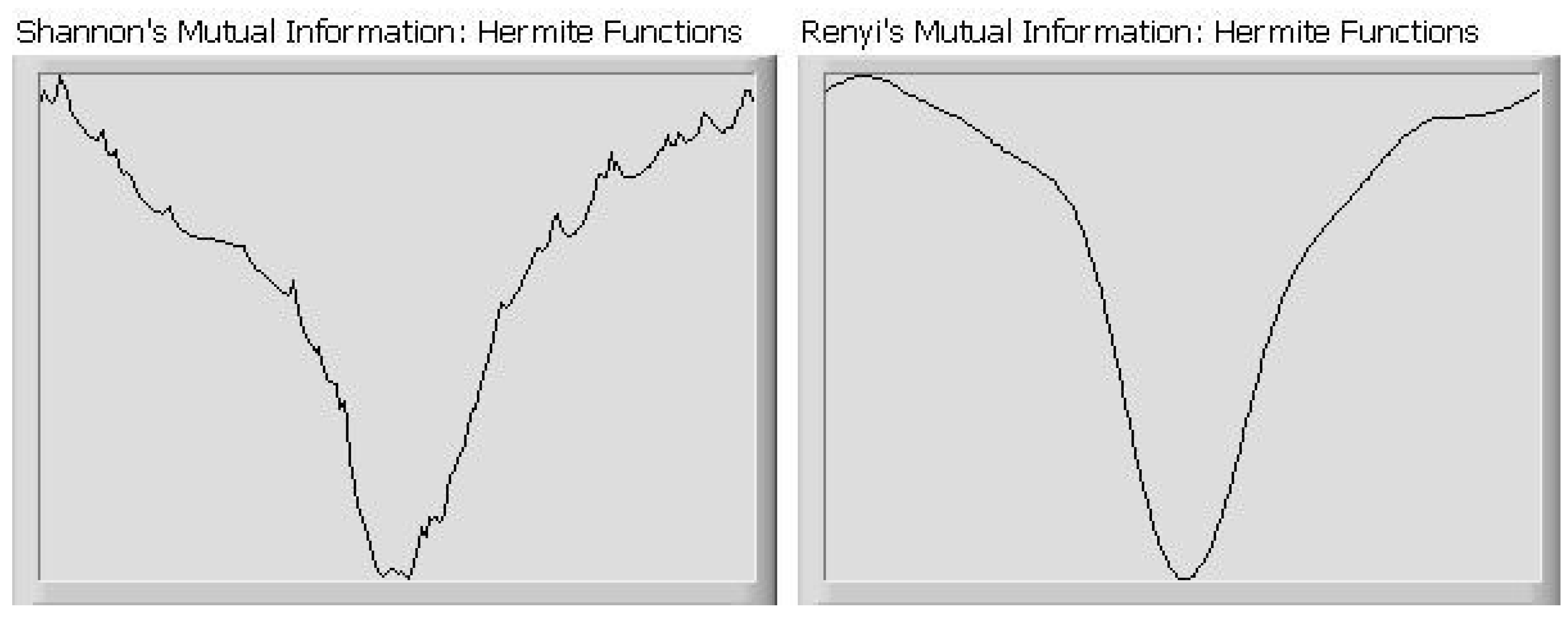
The mean Amari errors for each scenario can found in Table [2]; the last row containing the mean over all simulations. We can see that no-one method is superior or inferior to the rest. However, if we compare the mean of Amari’s error over all simulations, an estimate of Shannon’s mutual information based on kernel density estimators performs best. Also, using Hermite functions, ICA using Renyi’s mutual information works better than Shannon’s mutual information. A possible explanation for this is displayed in Figure [2]: the first graph displays the estimates of Shannon’s mutual information over a range of rotation matrices; the second graph displays estimates of Renyi’s mutual information for the same rotation matrices. Shannon’s and Renyi’s estimate of mutual information using Hermite functions displayed different behaviors, that is, Shannon’s was generally not that smooth compared to Renyi’s, leading to “false” minima. One possible reason for this can be seen in equation (9), where the absolute value of the estimated density is taken - the lack of smoothness in the absolute value function maybe transferred to the marginal entropy estimates.
We finish this section by comparing the time needed to calculate the various entropy estimates. One would expect that the Hermite function based estimates should be of order O ( n ) as they really only
Figure 2. Behavior of Shannon and Renyi Mutual Information Estimates using Hermite Functions
Entropy 10 00745 g002
Table 3. Calculation times for entropy calculation (milliseconds)
Shannon MI: HermiteRenyi MI: HermiteShannon MI: KernelRenyi MI: KernelRADICALFastICA
1000 points31244244540
2000 points524854851100
4000 points95378637862381
8000 points211014978149784852
involve one major summation; the kernel density based estimates should be of order O ( n 2 ) due to the double summation involved; the RADICAL estimate should be of order O ( n ) as it’s major component is sorting. Observations bear out these hypothesis - see Table [3], which contains the time in milliseconds taken to calculate the various entropy estimates for 1000, 2000, 4000 and 8000 data points. Moreover, we see that the Hermite based approximations are significantly faster than all but the FastICA estimate, which is to be expected as the FastICA does not involve many calculations.

4. Further Work

The complex-valued ICA case has not received the same attention as the real-valued case. Some ICA techniques have been developed for the case of sources with spherically symmetric distributions, that is, the distribution of a source is unchanged by the multiplication of e i θ . In this case, ICA techniques can be applied to the absolute value of un-mixed sources; both RADICAL and FastICA (see [2] and [11] respectively) have been extended to the complex case using this idea. Now, if the sources do not have spherically symmetric distributions, one cannot just consider the absolute value of the un-mixed sources. However, there is no reason why one cannot use the complex-valued versions of the information measures in equations (5) and (8). For both information measures, estimates of the entropy quantities making them up will be based on bi-variate density estimates; both Hermite series and kernel density estimates can give these. To illustrate, consider a bi-variate random variable ( X , Y ) with samples ( x i , y i ) i = 1 M . The Hermite series estimate of the bi-variate density p X , Y ( x , y ) is
p ^ X , Y ( x , y ) = m = 0 M n = 0 M b ^ n , m h m ( x ) h n ( y ) ,
where
b ^ n , m = i = 1 N h m ( x i ) h n ( y i ) .
The bi-variate versions of the entropy estimates in equations (9) and (10) are then
- 1 N i = 1 N log m = 0 M n = 0 M b ^ n , m h m ( x i ) h n ( y i ) ,
and
- log m = 0 M n = 0 M b ^ m , n 2 ,
respectively. Nonparametric density estimation using Hermite functions does have some advantages over kernel density estimation in higher dimensions. Firstly, as was noted in [15] and [16], the Hermite series estimate converges at the same rate (with respect to mean integrated square error and mean square error) regardless of dimension, whereas the rate of convergence of the kernel density based estimate degrades as the dimension increase. The second reason is that unlike the uni-variate case, it is a non-trivial task to choose the smoothing matrix required by the kernel density estimate.
Some further work would be to compare the performance of Hermite series and kernel density based estimates of the information measures in equations (5) and (8) for the case of complex data which is not spherically symmetric. In this case, the Hermite series approach may well prove to be superior due to it’s better scaling in multi-dimensions to that of kernel density estimates.

5. Conclusion

In this paper we have compared the performance of ICA using Hermite function based nonparametric estimates of Shannon’s and Renyi’s mutual information to that of kernel density based estimates, along with RADICAL and FastICA estimates of Shannon’s mutual information. In the eight scenarios considered, the Hermite function based approach was competitive in terms of performance with the other ICA approaches, and much faster to calculate than the kernel density based approach.

Acknowledgements

The authour would like to thank Prof. B. Moran for his valuable suggestions regarding the work in this paper.

References and Notes

  1. Amari, S.; Cichocki, A.; Yang, H. H. A new learning algorithm for blind signal separation. Advances in Neural Information Processing Systems 1996, 8, 757–763. [Google Scholar]
  2. Bingham, E.; Hyvarinen, A. A fast fixed-point algorithm for independent component analysis of complex-valued signals. Int. J. of Neural Syst. 2000, 10 (1), 1–8. [Google Scholar] [CrossRef]
  3. Boscolo, R.; Pan, H.; Roychowdhury, V. P. Independent component analysis based on nonparametric density estimation. IEEE Trans. Neural Networks. 2004, 55–65. [Google Scholar] [CrossRef]
  4. Como, P. Independent component analysis, A new concept? Signal Process. 1994, 287–314. [Google Scholar] [CrossRef] [Green Version]
  5. Erdogmus, D.; Hild II, K. E.; Principe, J. C. Independent components analysis using Renyi’s mutual information and Legendre density estimation. In Proceedings of International Joint Conference on Neural Networks, USA, July 2001, 4; pp. 2762–2767.
  6. Hild II, K. E.; Erdogmus, D.; Principe, J. C. Blind source separation using Renyi’s mutual information. IEEE Signal Process. Lett. 2001, 8, 174–176. [Google Scholar] [CrossRef]
  7. Hyvarinen, A. Fast and robust fixed-point algorithms for independent component analysis. IEEE Trans. Neural Networks. 1999, 10, 626–634. [Google Scholar] [CrossRef] [PubMed]
  8. Hyvarinen, A.; Karhunen, J.; Oja, E. Independent Component Analysis. John Wiley & Sons, 2001. [Google Scholar]
  9. Izenman, A.J. Recent developments in nonparametric density estimation. J. Amer. Statistical Assoc. 1991, 86, 205–223. [Google Scholar] [CrossRef]
  10. Learned-Miller, E. G.; Fisher III, J. W. ICA using spacing estimates of Entropy. J. Mach. Learn. Res. 2003, 4, 1271–1295. [Google Scholar]
  11. Lee, I.; Lee, T. Nonparameteric Independent Component Analysis for Circular Complex Variables. In Proceedings of IEEE International Conference on Acoustics, Speech and Signal Processing, Honolulu, 2007, 2; pp. 665–668.
  12. Obradovic, D.; Deco, B. Information maximization and independent component analysis: Is there a difference? Neural Computat. 2000, 2085–2101. [Google Scholar] [CrossRef]
  13. Parzen, E. On esimation of a probability density function and mode. Ann. Math. Statist. 1962, 33, 1065–1076. [Google Scholar] [CrossRef]
  14. Silverman, B. W. Density Estimation for Statistics and Data Analysis, Chapman and Hall. 1985. [Google Scholar]
  15. Schwartz, S. C. Estimation of a probability density by an orthogonal series. Ann. Math. Statist. 1966, 38, 1262–1265. [Google Scholar] [CrossRef]
  16. Walter, G. G. Properties of Hermite series estimation of probability density. Ann. Statist. 1977, 5, 1258–1264. [Google Scholar] [CrossRef]
  17. Webb, A. Statistical Pattern Recognition; Hodder Arnold, 1999. [Google Scholar]