Abstract
The paper is concerned with Shannon sampling reconstruction formulae of derivatives of bandlimited signals as well as of derivatives of their Hilbert transform, and their application to Boas-type formulae for higher order derivatives. The essential aim is to extend these results to non-bandlimited signals. Basic is the fact that by these extensions aliasing error terms must now be added to the bandlimited reconstruction formulae. These errors will be estimated in terms of the distance functional just introduced by the authors for the extensions of basic relations valid for bandlimited functions to larger function spaces. This approach can be regarded as a mathematical foundation of aliasing error analysis of many applications.
Keywords:
sampling formulae; differentiation formulae; non-bandlimited functions; aliasing error; Hilbert transforms; formulae with remainders; derivative-free error estimates; Bernstein’s inequality MSC Classification:
30H10; 41A17; 41A80; 42A38; 46E15; 65D25; 94A20; 26A16; 41A25; 44A15; 46E35
1. Introduction
According to Shannon’s sampling theorem, a signal , et al., a bandlimited signal (see Section 2 for the exact definition) can be completely reconstructed in terms of samples, equidistantly spaced apart the real axis . Likewise one can reconstruct the derivatives or the Hilbert transform and its derivative just in terms of samples of f. Almost immediate applications of these results are Boas-type formulae for arbitrary order derivatives of such signals as well as of their Hilbert transforms, used in numerical analysis for computation of those derivatives.
The essential aim is to extend these results to non-bandlimited signals, in fact to the largest class, denoted by below, for which the Fourier transform, the basic tool of this approach, can be employed effectively. Basic is the fact that by these extensions the exact reconstruction formulae have to be equipped with remainder (error) terms. The errors involved will be measured in terms of the distance of f from the space of bandlimited function, a concept just introduced by the authors for the extensions of basic relations for Bernstein spaces to larger function spaces.
To become familiar with the new approach, the classical Shannon sampling theorem for derivatives of -signals, namely Theorem 3.1 below, can be extended to the larger space by adding the remainder term of (6) to the expansion for bandlimited signals (5). This remainder, the aliasing error, can be estimated (cf. (7)) by:
The integral on the right-hand side is the above mentioned distance of from the space . Its behaviour depends on the smoothness properties of f, and was extensively studied in [1]. If f is bandlimited to , then it vanishes, as to be expected. Otherwise, if , the largest space to be considered in this context, then this distance tends to zero for . Furthermore, if one restricts the matter to certain subspaces of , one can obtain refined estimates, including unusually sharp rates of approximation; see Corollaries 3.5–3.7. In particular, if f belongs to a Lipschitz or Sobolev space, then decays like a negative power of σ, and if f belongs to a Hardy space, then it decays exponentially.
Similarly, to the sampling reconstruction for the derivatives of the Hilbert transform of -signals, thus for , namely (12), the remainder term of (14), must be added in order to obtain its extension (13) to . The remainder can be estimated in the same way as above.
The paper’s chief point is to generalize the Boas formula for the first derivative, namely (16), to higher order ones, odd order given by (25), even orders by (26). Thus, e.g., the derivative is expressed in terms of the signal values , which depend however on . The proof is unusually simple, one just sets and in Theorem 3.1 and applies the resulting formula to the function .
For the first major result, Theorem 5.1, the extension of (25) to the larger class , formula (25) has to be equipped with the aliasing error term of (38), which can be estimated in the same fashion as the error above, which again tends to zero for .
A basic inequality in the theory of functions of exponential type is Bernstein’s inequality for the derivatives for bandlimited f in the finite energy norm or in , . This result is generalized in Section 6 to non-bandlimited signals, the aliasing error being (52) in the case of odd order derivatives and (53) for even ones.
2. Notation and Preliminary Results
As usual, is the space of all real or complex-valued function f that are Lebesgue integrable to the pth power over the real axis , endowed with the norm , , and is the space of all measurable essentially bounded functions f with the norm . By we denote the class of all functions that are uniformly continuous and bounded on , where .
The Fourier transform of , , is defined by:
where . If , , is such that , then there holds the Fourier inversion formula:
at each point where f is continuous; see [2, Proposition 5.1.10, 5.2.16].
For and , let the Bernstein space comprising all entire functions (thus arbitrary often differentiable) of exponential type σ, (i.e., for , which belong to when restricted to the real axis . There holds:
According to the Paley–Wiener theorem (cf. [3, p. 103]), a signal f belongs to ; , if and only if it is bandlimited to , i.e., its Fourier transform vanishes outside . The same holds true for , if the Fourier transform is understood in the distributional sense. Note that a bandlimited signal cannot be simultaneously duration limited.
The sinc function is defined by:
where the rectangle function is given by:
Moreover, there holds by the Fourier inversion formula (1) (cf. [2, Section 5.2.4]):
2.1. A Hierarchy of Spaces Extending Bernstein Spaces
In order to extend the Bernstein space to larger function spaces, we weaken the property of f being bandlimited, vanishes outside the compact interval , to belonging to . This still guarantees the reconstructibility of f from its Fourier transform in terms of the inversion formula (1). To this end, we introduce the Fourier inversion classes:
For , there holds . In addition to (1) one has for that the derivative exists, belongs to and has the representation:
see [2, Proposition 5.1.17 with replaced by ].
The Fourier inversion classes are in some sense the most general spaces in which our studies can be performed. Spaces between and are also of interest since they will yield smaller errors in the extended formulae.
The modulus of smoothness of of order is defined by:
and the associated Lipschitz class for by:
The Sobolev space is given by:
and Hardy spaces for horizontal strips , , by:
There hold the inclusions:
Here we recall some facts concerning the distance functional introduced in [1]. Let G be the vector space of all functions having the representation:
for some . We define the distance of two functions having representation (4) with , respectively, by:
and the distance of a functions from the Bernstein space by:
If , , then the derivative belongs to G with . Hence one has for with , ,
Moreover, one has for , ,
Observe that for and one has in view of the isometry of the Fourier transform that , i.e., is the Euclidean distance.
The following estimates for the distance can be found in [1]. In each of the subsequent statements, c and γ with attached indices denote positive numbers that depend only on the indices but not on f and σ. They may be different at each occurrence.
Proposition 2.1.
(a) Let with , , and . One has the derivative free estimate:
If also , , then:
If , , , then:
(b) If and , , , then for each ,
the latter holding provided , .
Proposition 2.2.
Let . Then, for , , and ,
Proposition 2.3.
Let . Then, for , ,
3. Extensions of Shannon’s Theorem to Non-Bandlimited Signals and Their Hilbert Transforms; Aliasing Errors
Let us consider the well-known Whittaker–Kotel’nikov–Shannon sampling theorem for reconstructing a bandlimited signal and its derivatives in terms of samples of just f, namely ((see e.g., [4,5], [6, p. 13], [7, p. 59]).
Theorem 3.1.
Let , then, for each ,
the series converging absolutely and uniformly for as well as in -norm.
This theorem can be extended to the larger space by adding a remainder or error term , to the expansion (5). This leads to the following extended version of Theorem 3.1.
Theorem 3.2.
Let for some , and let be the 2π-periodic signal, defined for by:
Then one has the approximate sampling representation:
with the remainder given by:
In particular, there holds:
The remainder is the so-called aliasing error occurring when a non-bandlimited signal is reconstructed in terms of the sampling theorem; see e.g., [8].
The case can be found already in [9] (see also [5,7,10]), [6, p. 15 ff]), where the remainder (6) was given in the equivalent form:
Theorem 3.2 for arbitrary is contained in [11], where it was deduced as a particular case of a unified approach to various sampling representations. This general approach also covers the following two results on the reconstruction of the Hilbert transform and its derivatives in terms of samples of f; see [5,11].
The Hilbert transform or conjugate function of , defined by the Cauchy principal value:
plays an important role in electrical engineering (see [12, p. 267 ff.], [13]). For the Hilbert transform, also often called “one of the most important operators in analysis”, one may consult [2, Chap. 8, 9], [14,15]. It defines a bounded linear operator from into itself, and one has:
Furthermore, if for some , then by the Fourier inversion formula Equation (1) for each ,
the latter equality holding provided . This formula also shows that ; thus derivation and taking Hilbert transform are commutative operations.
Noting (2) and (8), we see that the Fourier transform of the Hilbert transform of the sinc-function is given by:
and one easily obtains from the case in (9) that the Hilbert transform of the sinc-function is given by:
Moreover, one has the representation:
Since the Hilbert transform is a bounded linear operator from into itself, which commutes with differentiation, the following sampling representation follows immediately from (5) by taking the Hilbert transform of each side.
Theorem 3.3.
Let , where . Then, for each ,
the series converging absolutely and uniformly for as well as in -norm.
This formula enables one to compute in term of samples of f itself; for the case see [5,6,7,16], and for arbitrary s see [11]. The extended version of this result reads (see [11]):
Theorem 3.4.
Let for some , and let be the 2 t by:
Then one has the approximate sampling representation:
with the remainder given by:
In particular, there holds:
The integral on the right-hand side of (7) and (15) is the distance of from the space . Its behaviour for depends on the smoothness properties of f, and was extensively studied in [1]; recall Section 2.1. This leads to the following estimates for the remainders and .
Corollary 3.5.
If , , then for any and ,
In particular, if in addition for , then:
Corollary 3.6.
Let , for some . Then: for ,
If moreover , , then
Corollary 3.7.
If , then for , positive , and ,
The three corollaries remain true, if is replaced by .
4. Boas-type Formulae for Higher Derivatives
In [17] (see also [3]) Boas established a differentiation formula that may be presented as follows.
Let , where . Then, for , we have:
When f is a trigonometric polynomial of degree n, i.e., , then and so (16) applies. In this case, by virtue of the periodicity of f, the series in (16) can be condensed to a finite sum. The resulting formula was obtained by M. Riesz in 1914 [18]. In fact, Riesz’s interpolation formula for trigonometric polynomials reads:
where and for . Since , (17) implies the classical Bernstein inequality:
Analogously to the proof of (18), Boas’ formula (16), also known as generalized Riesz interpolation formula (as Isaac Pesenson informed us), can be used to prove the basic Bernstein inequality for functions , namely , , which will be treated extensively in Section 6.
There exist families of differentiation formulae for higher derivatives holding in Bernstein spaces; see [6, § 3.2]. Which of them should we consider as a generalization of Boas’ formula? In the applications of (16) the following properties are crucial:
- (a)
- The formula applies to all entire functions of exponential type σ that are only bounded on .
- (b)
- The sample points are uniformly spaced according to the Nyquist rate and are located relatively to the argument t of the derivative.
- (c)
- The coefficients do not depend on t.
- (d)
- The coefficients decay like as .
- (e)
- When the sample points are arranged in increasing order, then the associated coefficients have alternating signs.
In the case of higher derivatives, a Boas-type formula should also have the properties (a) to (e).
The Boas-type formulae to be established will be deduced as applications of the Whittaker–Kotel’nikov–Shannon sampling theorem for higher order derivatives (Theorem 3.1). Another approach by contour integration methods of complex function theory will be presented in Section 4.1.
In view of Leibniz’s rule, the basic term in (5) can be written as follows:
Expressing now in terms of and , we can rewrite in the more handy form:
where the right hand side is naturally thought to be continuously extended at by:
This can be easily obtained from (3) or the power series expansion:
Further, it follows easily from (19) that:
In view of (3) there holds the Fourier expansion (cf. [2, Proposition 4.1.5]):
and, in particular, for and ,
As an application, we now come to two Boas-type formulae, one for derivatives of odd order and one for those of even order.
Theorem 4.1.
Let for some , and define for ,
Then there hold the representations:
Proof.
The identities (23) and (24) follow immediately from (19), noting that and .
For (25) and (26) we will give two proofs. The first one applies only to , which seems to be the more interesting case in engineering applications, whereas the second one also covers the larger space .
First assume that , i.e., . Setting in (5), then by the definition of ,
Now, if for arbitrary , then (25) follows by applying (27) to the function , which belongs to .
For even order derivatives, one obtains from (5) for and ,
The proof can now completed along the same lines as in the case of odd order derivatives.
In order to extend (25) and (26) to , one may apply the -result just proved to the function , , which belongs to , and then let . This density argument can be avoided by the following alternative proof. To this end, let , and let be defined by:
By Leibniz’s rule one has:
Since , we can apply (5) to the terms on the right-hand side to obtain:
Now, we have to distinguish between odd and even order derivatives. Replacing s by and setting in (28), we obtain in view of (20),
Further, noting (22) and the definition of , we end up with:
To complete the proof for odd order derivatives, let now for arbitrary and apply (29) to the function , where .
For even order derivatives one starts again with (28), replaces s by and sets . In view of (21), (22) and (24), one then obtains:
Finally, apply this equation to the function . ☐
Representation (25) can also be found in [19, Corollary 5], where it was proved by contour integral methods.
For , (25) is the classical Boas formula (16), and (26) reads:
The case in (25) gives:
It is easily seen that formulae (25) and (26) both have the properties (a) to (d), but it is not immediately clear whether (e) holds. We need to know the signs of the numbers and . For this, we represent these numbers by an integral with an integrand that does not change sign.
Proposition 4.2.
(a) For , the numbers of (23) have the representation:
In particular,
(b) For the numbers of (24) have the representation:
In particular,
Proof.
First we note that the sum on the right-hand side of (23) is the Taylor polynomial of the cosine function of degree with respect to the origin, evaluated at . Next we recall Taylor’s formula for a function f with the remainder represented by an integral. It states that:
see, e.g., [20, p. 88, Theorem 6]. Applying this formula to with , we see that (23) may be rewritten as:
By a change of variables, we obtain:
Now an integration by parts, taking as a primitive of , yields:
for . From this, (30) follows immediately.
Except for a set of measure zero, the integrand in (30) is positive on the interval of integration if the upper limit of the integral is positive, and is negative if that limit is negative. This shows that the integral in (30) is always positive. Hence (31) holds for , and in view of for as well.
Regarding (32), we note that the sum on the right-hand side of (24) is the Taylor polynomial of degree of the sine function evaluated at . Using again (34) and proceeding as in the proof of (a), we arrive at (32) and (33). ☐
Now (31) and (33) show that formulae (25) and (26) have also the property (e) and so they are Boas-type formulae in our sense.
One may ask, why we started with in the proof of (25), and with in the proof of (26). If one begins with in the case of odd order derivatives, one would end up with formulae, the coefficients of which behave like for . Moreover, they are valid in for only, but not in . Hence they are not Boas-type formulae in our sense. For such a formula can be found in [7, p. 60 (87)].
4.1. An Alternative Approach by Methods of Complex Analysis
Formulae (25) and (26) of Theorem 4.1 can also be derived by contour integration without employing the sampling theorem and without requiring a process that leads from to .
Denote by the positively oriented rectangle with vertices at For , we first consider the meromorphic function:
It has a simple pole or a removable singularity at for , a pole of order at most at zero and no other singularities. Noting that the sum is a truncated Taylor expansion of around , we conclude that:
By a well-known formula for the residue at a pole of order at most , this implies that:
Furthermore, it is easily verified that:
with given by (23).
Now, for , it is readily seen that:
Hence by the residue theorem,
which implies (25) by a transformation of the argument of f.
Analogously, one considers:
Here is a pole of order at most and,
which gives:
while,
with given by (24). This time, for , we find that:
which implies (26) by a transformation of the argument of f.
4.2. Variants
If we abandon property (e) of a Boas-type formula and admit a correction at t by the value of f or that of its first derivative, we can improve upon property (d) by establishing formulae with coefficients that decay like as . Such formulae are of interest in numerical applications since the truncated series will need less terms for achieving certain accuracy.
The following formula (35) was already obtained in [19, Corollary 5] by methods of complex analysis; formula (36) is new.
Corollary 4.3.
Let for some and let . Then, in the notation of Theorem 4.1,
Proof.
Obviously the function belongs to and, as is seen by Taylor expansion around 0, we have
Thus applying (25) to g at , we obtain
For this formula holds with and yields
Thus,
which gives (35) by shifting the argument of f.
Analogously, applying (26) to g at , we obtain:
For the sinc function, this formula holds with and yields:
Thus,
which gives (36) by substituting the value of and shifting the argument of f. ☐
5. Extensions to Non-Bandlimited Functions
Theorem 5.1.
Let . Then exists, and for , formula (25) extends to:
where,
being the -periodic function defined by:
In particular,
Proof.
First assume , i.e., , and let:
Then and so (25) applies to this difference, i.e.,
and we find that for ,
>From (41) there follows:
and,
When we use these expressions for the calculation of (42), an interchange of summation and integration is permitted by Levi’s theorem. Hence,
Consider now the function . Obviously when , and so (25) applies to for these values of v, i.e., for ,
This means that:
Noting that the left-hand side of (44) is a -periodic function satisfying, in addition,
we see from the definition (39) of that (44) even holds for all , and inserting this into (43),we now obtain (37) with remainder (38) for and .
For arbitrary and one applies this particular case to the function . Since , the general form (38) of the remainder now follows by a change of variable.
Since for all , the first relation in (40) follows immediately. The second is a consequence of [1, Proposition 15]. ☐
Theorem 5.2.
Let , . Then exists and for , formula (26) extends to:
where,
being the -periodic function defined by:
In particular,
Proof.
We proceed as in the proof of Theorem 5.1. With as defined by (41) we have:
Noting that,
it follows that,
Applying now (26) to , where , we find:
which yields (45) and (46) for and . The general case follows again by applying this particular case to .
Since is a -periodic function, we have for all . This yields the first relation in (47), and the second one is again a consequence of [1,Proposition 15]. ☐
Counterparts of Corollaries 3.5–3.7 are also valid in the instance of the error .
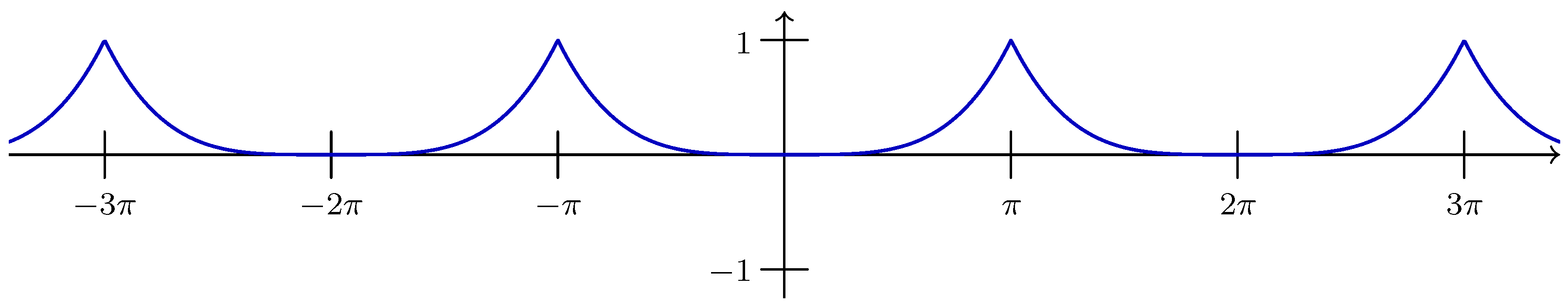
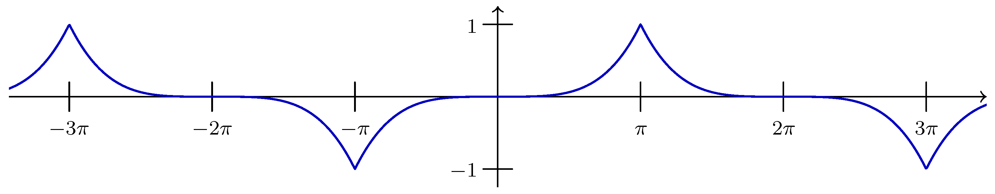
For , Theorem 5.1 reduces to [1, Theorem 5]. The graphs of , , , are shown in Figure 1, Figure 2, Figure 3 and Figure 4, respectively.
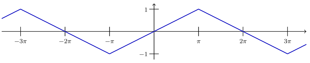
Figure 1.
The graph of .
Figure 1.
The graph of .
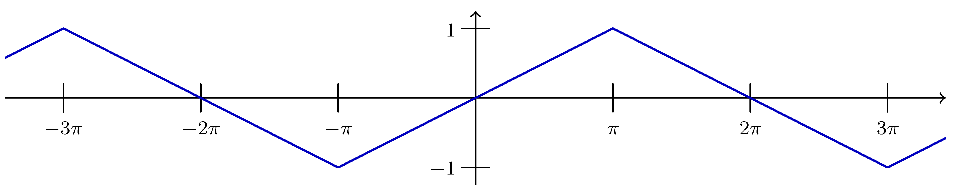
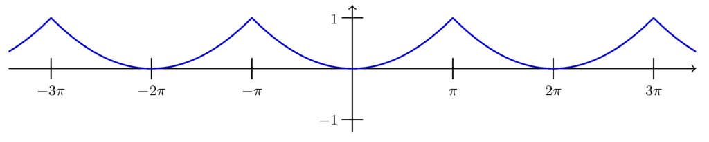
Figure 2.
The graph of .
Figure 2.
The graph of .
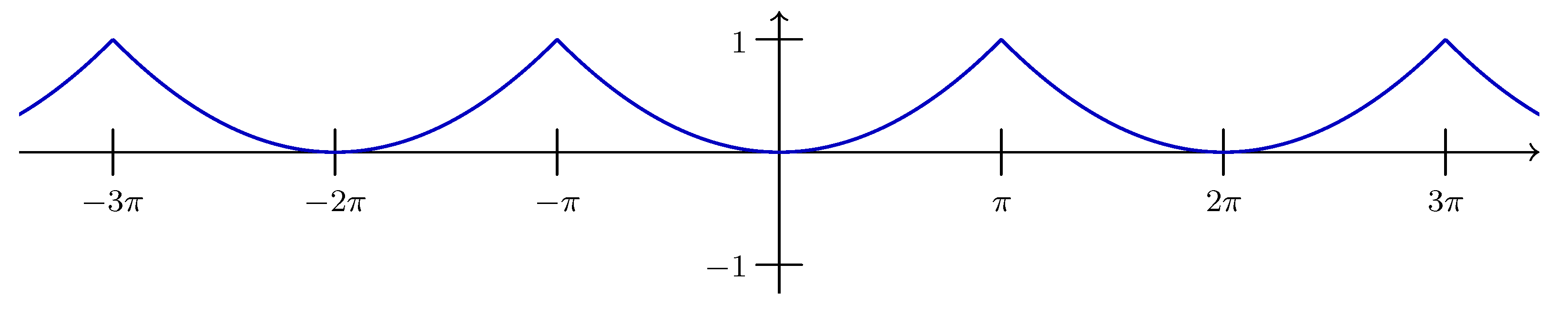
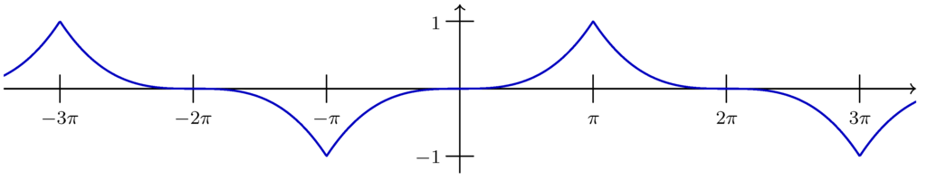
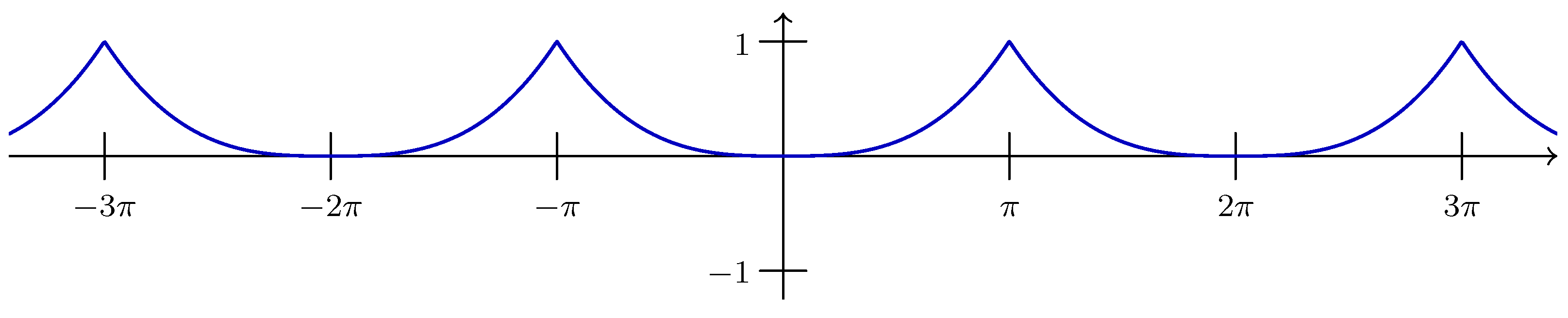
Figure 3.
The graph of .
Figure 3.
The graph of .

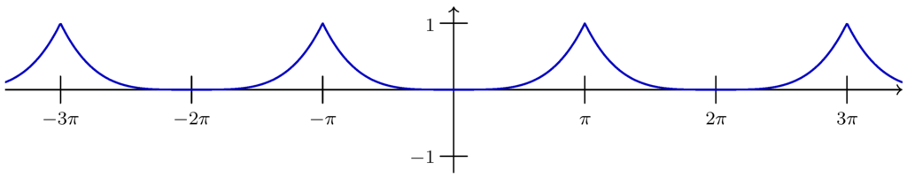
Figure 4.
The graph of .
Figure 4.
The graph of .
6. Extended Bernstein Inequalities for Higher Order Derivatives
We now come the matter sketched at the beginning of Section 4. The well-known Bernstein inequality states:
For , , , there holds:
The case is usually proved with help of Boas’ formula (16), and the general case then by iteration; see [3, Section 11.3]. Boas’ formulae for higher order derivatives enables us now to prove (48) directly for arbitrary . Indeed, we have by (25),
The series on the right-hand side can be evaluated as follows. Since , formula (25) applies to this function. For it yields that:
where (31) has been used in the last step. Combining this equation with (49), we obtain (48). For derivatives of even order one uses (26) and proceeds analogously.
In this section we employ Theorems 5.1 and 5.2 to extend Bernstein’s inequality for higher derivatives to non-bandlimited functions by adding an “error term”. For this aim, properties (a)–(e) of a Boas-type formula, specified in Section 4, will be crucial.
Theorem 6.1.
Let , , , and suppose that belongs to as a function of v. Then, for any , we have:
with defined by (38). Furthermore,
Proof.
Consider (37) as a function of t and apply on both sides. Using the triangle inequality on the right-hand side and noting that does not change under a shift of the argument of f, we find that:
Inserting (50) for the series on the right-hand side, we obtain (51).
Next we observe that is the Fourier transform of the function:
The hypotheses imply that . Thus, using [2, Prop. 5.2.6] and noting that this book uses the notation , we conclude that:
where we have used that . This completes the proof. ☐
By an analogous proof, we deduce from Theorem 5.2 the following result for derivatives of even order.
Theorem 6.2.
Let , , , and suppose that belongs to as a function of v. Then, for any , we have:
with defined by (45). Furthermore,
It should be noted that for derivatives of odd order the bound in terms of the distance function is by a factor bigger than the corresponding bound for derivatives of even order. However, when , we can profit from the isometry of the Fourier transform and deduce the same bound in both cases. An obvious modification of the proof in [1,Theorem 11] leads to the following result.
Theorem 6.3.
Let , and suppose that as a function of v. Then, for any , we have
7. Landau–Kolmogorov Inequalities
In this section we consider the case where f belongs to a Sobolev space and deduce Landau–Kolmogorov inequalities, a very popular and still active field. The proof of the following proposition is essentially contained in that of [1, Proposition 13].
Proposition 7.1.
Let , where . Then for with , we have
and
for and , where
Proposition 7.1 enables us to deduce from Theorems 6.1–6.3 the following corollaries.
Corollary 7.2.
Let and , where . Then, for and any , we have:
Corollary 7.3.
Let and let , where . Then, for and any , we have
Corollary 7.4.
Let and let , where . Then, for any , we have:
Note that for Corollary 7.2 reduces to a result in [1, Corollary 16].
The statements of Corollaries 7.2–7.4 can be interpreted as a linearized equivalent form of a Landau–Kolmogorov inequality [21,22]. The equivalence is shown by the following lemma in which . A more specialized result was mentioned by Stečkin [23]; also see [21, pp. 5–6].
Lemma 7.5.
Let and Then,
for all if and only if,
where,
Proof.
Suppose that (58) holds. Then we may minimize the right-hand side over σ by using standard calculus. This leads us to (59) with α and K given by Equation (60).
Conversely, suppose that (59) holds with and . Consider now the function:
Its Hessian shows that it is concave on . Hence, at any point the tangent plane of F lies above the graph of F, that is,
Setting , we find by a straightforward calculation that:
Now, setting and defining:
we find that:
This shows that:
with C defined by (60). Since λ may take any value in , the same is true for σ. Hence (59) implies (58). ☐
Lemma 7.5 can be used to deduce three Landau–Kolmogorov inequalities from (55)–(57). We may state them in a unified form as follows.
Corollary 7.6.
Let and , where and For define:
and,
with given by (54). Then,
Unfortunately, the constant in (61) is not the best possible. However, the discussion in [24, pp. 442–447], does not extend to results for . For inequality (61) simplifies to:
Here the term in square brackets can be replaced by 1. For and , this is shown in [25, § 7.9, No. 261]. For general with , we may use the isometry of the -Fourier transform together with Hölder’s inequality and proceed as follows:
Now, employing Lemma 7.5, we may in turn improve upon Corollary 7.4. This way we obtain:
Corollary 7.7.
Let and let , where . Then, for any , we have
8. Boas-type Formulae for the Hilbert Transform
We now establish the counterparts of the theorems of Section 4 and Section 5 in the instance of Hilbert transforms. Although the definition of the Hilbert transform can be extended to signals , , (see [26, p. 126 ff.]), we restrict ourselves to the most important case .
8.1. Formulae for Bandlimited Functions
The derivatives are needed. They are given by (cf. (10)),
By the cosine addition formula this can be rewritten as:
where the right hand side is thought to be continuously extended at by:
This can be easily obtained from (11) or the power series expansion:
As an application, we now come two new Boas-type formulae, one for derivatives of odd order and another for those of even order.
Theorem 8.1.
Let for some and . Then for ,
and for ,
Here the coefficients and are given by:
Proof.
The proof follows along the same lines as the first proof of Theorem 4.1, starting with:
in the case of odd order derivatives, and with:
for even orders. ☐
For one obtains from (64):
and the case in (63) gives:
already to be found in [27, p. 203]; see also [11]. The case in (64) gives:
8.2. Achieser-type Formulae
Achieser [26, p. 143, (II)] proved an informative formula, which combines the assertions of the first derivative of a signal and that of its Hilbert transform. It may be stated for our definition of the Hilbert transform as follows:
Let . Then,
We now establish analogous formulae for higher derivatives, distinguishing the cases of odd and even order.
Theorem 8.2.
Let for some and . Then for and ,
and,
where,
and,
Proof.
First let Then,
By using the formulae (19) and (62) for calculating the term in square brackets, we find that:
for with as defined in the theorem. The values of and show that the left-hand side is equal to the right-hand side for as well. Hence we have proved that:
If for an arbitrary , then applying this result to the function , we obtain (69). The proof of (70) is strictly analogous. ☐
Remark 8.3.
Note that Theorem 8.2 contains the statements of Theorems 4.1 for and 8.1 for as special cases. This follows by observing that:
Next we establish integral representations for the numbers and , which allow us to determine the signs of these numbers.
Proposition 8.4.
(a) For , and we have the integral represention:
Furthermore,
for all and
(b) For and we have the integral representation:
Furthermore,
for all , and
Proof.
Let and . Writing as and using Taylor’s formula as given by (34), we readily find that:
Now integration by parts and a change of variables yields (71). The integral in (71) is always positive, regardless of whether is positive or negative. This shows that (72) holds whenever (71) is valid. For and for the exceptional values of α, the validity of (72) can be verified directly.
The proofs of (73) and (74) are analogous except for obvious variations. ☐
8.3. Extensions to Non-bandlimited Functions
Our next aim is to extend (63) and (64) to larger function spaces.
Theorem 8.5.
Let . Then exists and for , formula (63) extends to:
where,
with being the -periodic function defined by:
In particular,
Proof.
Following the proof of Theorem 5.1 we find that:
and,
There follows:
In order to evaluate the infinite series in (76), we have to proceed in a different way from the proof of Theorem 5.1. Indeed, since the function does not belong to we cannot apply formula (63) to this function.
On the other hand, there holds by (65) and (11),
i.e., the series in (76) is the (trigonometric) Fourier series of the -periodic function with defined by (75). Moreover, since is differentiable, save possibly for , , we even have (cf. [2, Proposition 4.1.5]),
The proof can now be completed as the proof of Theorem 5.1. ☐
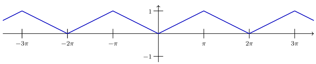
Figure 5.
The graph of .
Figure 5.
The graph of .
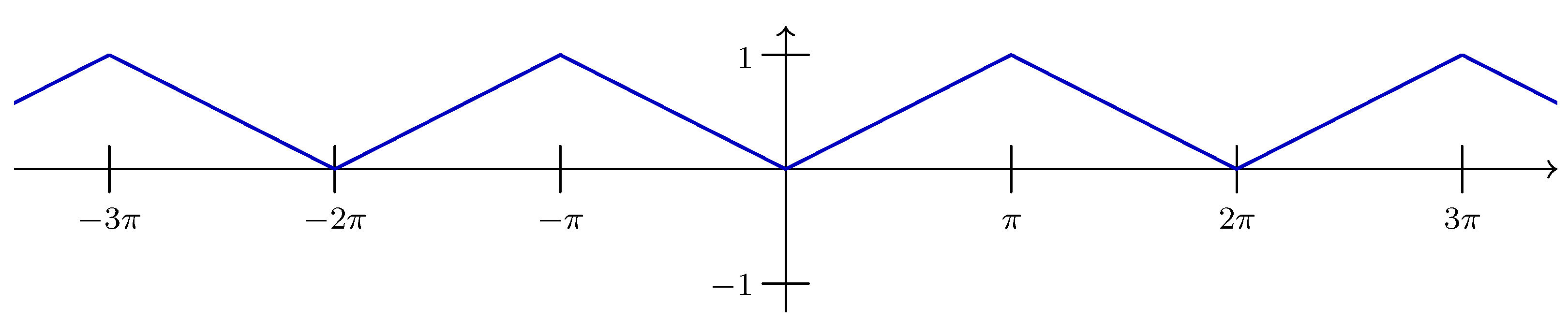
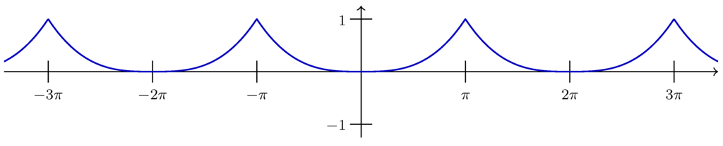
Figure 6.
The graph of .
Figure 6.
The graph of .
Theorem 8.6.
Let , . Then exists and for , formula (64) extends to:
where,
Here is the -periodic function defined by:
In particular,
Proof.
Proceeding as in the proof of Theorem 8.5, we arrive at a formula corresponding to (76), namely,
Noting (66) and (11), we see that the infinite series in (79) can be rewritten as a Fourier series, namely,
and, using the same arguments on the convergence of Fourier series as above, we obtain:
Since the series in (80) defines a -periodic function satisfying for all , it follows that (80) holds a. e. on . This yields (77) with remainder (78) for and . The rest of the proof now follows as in the proof of Theorem 5.1. ☐
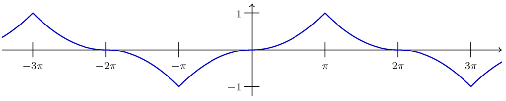
Figure 7.
The graph of .
Figure 7.
The graph of .
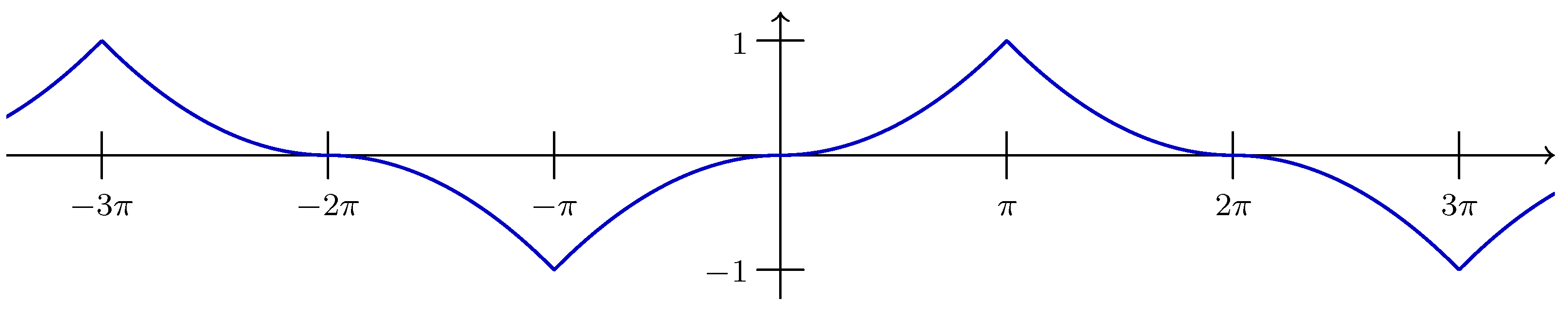
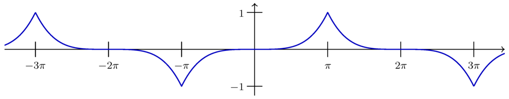
Figure 8.
The graph of .
Figure 8.
The graph of .
9. Applications
In this section we apply the results of Section 3 and Section 8 to the signal function , , having Fourier transform and Hilbert transform . The extended sampling theorem for the Hilbert transform (Theorem 3.4) takes on the concrete form, first for ,
In practice, one has to deal with a finite sum rather than with the infinite series. This leads to an additional truncation error, namely,
Assuming for some constant , then the terms of the latter series, denoted by , can be estimated by:
This yields for the truncation error:
Combining the aliasing error in (81) with this estimate for the truncation error, we finally obtain:
Thus, we have a pretty precise and practical estimate for the error occurring when the derivative of the Hilbert transform is reconstructed in terms of the Hilbert version of the sampling theorem. Whereas the first term on the right-hand side covers the aliasing error, the second one is due to truncation.
Similarly, the Boas-type theorem for higher order derivatives (Theorem 8.5) takes the form (recall (67)):
For the second order derivative of one obtains from Theorem 8.6 for ,
These are the aliasing errors for the reconstruction of derivatives of the Hilbert transform in terms of the Boas-type formulae. In both cases, the truncation errors can be handled in a similar fashion as above.
Acknowledgements
The authors would like to thank Mikael Skoglund, guest editor together with Eduard Jorswieck of the present special issue of Entropy to which the authors were invited to contribute, for his help on the details concerning Willy Wagner’s many honours received from Sweden.
They also would like to thank Jörg Vautz, Lehrstuhl A für Mathematik, RWTH Aachen, for carefully preparing the eight figures.
A Brief Biography of Karl Willy Wagner
Karl Willy Wagner, born in Friedrichsdorf, a town in the Taunus founded 1687 by the Huguenots (his mother Emilie Zeline, née Gauterin, was a traditional Huguenot), who completed his studies as an electrical engineer at the well-known Technikum Bingen in 1902, worked in 1904–1908 as a research engineer at Berlin’s Siemens & Schuckert. In 1908 he became the assistant to the physicist Hermann Theodor Simon at Göttingen under whom he received his Dr. Phil. in 1910, and in 1912 he earned the Habilitation degree at the TH Berlin. Already in fall 1912 he was appointed Professor and member of the Physikalisch-Technische Reichsanstalt, and its President from 1923 to 1927. Then he became the founding professor of the Institute für Schwingungsforschung (Oscillation Theory) at the TH Berlin, named the Heinrich-Hertz-Institute in 1930.
At a special meeting of the Heinrich-Hertz Institute of January 1936 the Gaudozentenführer (the Nazi boss of Berlin’s universities), Willi Willing (1907–1983), reported that he planned to dismiss Wagner from his offices due to certain financial irregularities: allegedly receiving a Leica camera from the Leitz firm and for driving home in his official car in a roundabout way for coffee. None of the professors present objected, only Dr. Alfred Thoma, Wagner’s assistant, did, stating that these accusations did not represent the facts. As a consequence, he was discharged a few day later. Willing declared Wagner a Volksfeind (state enemy) and fired him.
Willing himself, who had received his doctorate only in 1935, became provisional Director of the Heinrich-Hertz Institute that February 1936.
According to Wagner himself, he was removed from office because he refused to dismiss his Jewish employees, ignoring the Nuremberg laws of September 1935 according to which German universities were to be “cleansed” of their Jewish students and lecturers.
As Dr. Thoma reported, Wagner would have been sent to a concentration camp, if he had not been bedridden with thrombosis at the time. Until 1938 most prisoners of concentration camps, which were an integral feature of the regime as soon as Hitler came to power, and were established all over Germany to handle the masses of people labelled as political/religious opponents and social deviants, were German citizens. Only after the “Kristallnacht” pogroms of November 1938 did the Nazis conduct mass arrests of adult male Jews. To facilitate the genocide of the Jews, the Nazis established “killing centers”, the first being Chelmno in Poland in December 1941.
After his dismissal Wagner returned home to Friedrichsdorf and together with his brother-in-law Friedrich Schmitt founded the “Landgrafen-Zwiebackfabrik”, enabling him to make a living.
In 1949 Wagner became President of the predecessor of the University of Mainz, which he co-founded, and in 1951 became Honorary Professor at Mainz.
He received many honours, the first, in 1919, being the “Cedergrenska guldmedaljen” (Gold Cedergren Medal), awarded every five years by the Royal Institute of Technology in Stockholm, and in 1935 he was elected a corresponding member of the Royal Swedish Academy of Engineering Sciences (korresponderande ledamot Kungl. Ingenjörsvetenskapsakademin) there. He was a referee of Wilhelm Cauer’s milestone thesis of 1926. Already in the fall of 1946, Wagner could again visit his colleagues in Switzerland. A little later, he was invited to lecture in Stockholm, Uppsala and Gothenburg, as well as to a guest-course at the KTH, the Royal Institute of Technology at Stockholm. Wagner’s treatise “Operatorenrechnung und Laplace Transformation” [28] was one of the first to attempt a justification of the operational calculus of Oliver Heaviside (the recipient of the Cedergren Medal in 1924), as well as to make transform methods popular in engineering circles, Fourier transforms being one of them; see [29,30,31,32,33].
Our paper is therefore dedicated to a true man of principles, a renowned electrical engineer, one who was fired from office for not having dismissed his Jewish employees, one of few such cases known in university circles during Nazi times.
References
- Butzer, P.L.; Schmeisser, G.; Stens, R.L. Basic relations valid for the Bernstein space and their extensions to functions from larger spaces in terms of their distances from . To be submitted for publication.
- Butzer, P.L.; Nessel, R.J. Fourier Analysis and Approximation; Academic Press: New York, NY, USA; Birkhäuser: Basel, Switzerland, 1971. [Google Scholar]
- Boas, R.P., Jr. Entire Functions; Academic Press Inc.: New York, NY, USA, 1954. [Google Scholar]
- Lundin, L.; Stenger, F. Cardinal-type approximations of a function and its derivatives. SIAM J. Math. Anal. 1979, 10, 139–160. [Google Scholar] [CrossRef]
- Butzer, P.L.; Splettstößer, W. Approximation und Interpolation durch verallgemeinerte Abtastsummen; Westdeutscher Verlag: Opladen, Germany, 1977. [Google Scholar]
- Butzer, P.L.; Splettstößer, W.; Stens, R.L. The sampling theorem and linear prediction in signal analysis. Jahresber. Deutsch. Math.-Verein. 1988; 90, 19–70. [Google Scholar]
- Butzer, P.L.; Schmeisser, G.; Stens, R.L. An Introduction to Sampling Analysis. In Nonuniform Sampling—Thery and Practice; Marvasti, F., Ed.; Kluwer/Plenum: New York, NY, USA, 2001; pp. 17–121. [Google Scholar]
- Splettstößer, W. 75 Years of Aliasing Error in the Sampling Theorem. In EUSIPCO–83, Signal Processing: Theories and Applications, Proceedings of the 2nd European Signal Processing Conference, Erlangen, Germany, 12–16 September 1983; Schüssler, H.W., Ed.; North-Holland Publishing Company: Amsterdam, The Netherlands, 1983; pp. 1–4. [Google Scholar]
- Brown, J.L., Jr. On the error in reconstructing a non-bandlimited function by means of the bandpass sampling theorem.
- Butzer, P.L.; Splettstößer, W. A sampling theorem for duration-limited functions with error estimates. Inf. Control 1977, 34, 55–65. [Google Scholar] [CrossRef]
- Stens, R.L. A unified approach to sampling theorems for derivatives and Hilbert transforms. Signal Process 1983, 5, 139–151. [Google Scholar] [CrossRef]
- Bracewell, R.N. The Fourier Transform and its Applications, 2nd ed.; McGraw-Hill Book Co.: New York, NY, USA, 1978. [Google Scholar]
- Boche, H. Charakterisierung der Systeme zur Ermittlung der Hilbert-Transformation (in German with English summary) [Characterization of systems to calculate the Hilbert-Transform]. Forschung im Ingenieurwesen 1997, 63, 1–6. [Google Scholar] [CrossRef]
- Hahn, S.L. Hilbert Transforms in Signal Processing; The Artech House Signal Processing Library, Artech House Inc.: Boston, MA, USA, 1996. [Google Scholar]
- Feldman, M. Hilbert Transform Applications in Mechanical Vibration; John Wiley & Sons: New York, NY, USA, 2011. [Google Scholar]
- Boche, H. Konvergenzverhalten der konjugierten Shannonschen Abtastreihe (in German with English summary) [Convergence behavior of the conjugate Shannon sampling series]. Acta Math. Inform. Univ. Ostraviensis 1997, 5, 13–26. [Google Scholar]
- Boas, R.P., Jr. The derivative of a trigonometric integral. J. Lond. Math. Soc. 1937; S1–S12, 164. [Google Scholar]
- Riesz, M. Eine trigonometrische Interpolationsformel und einige Ungleichungen für Polynome. Jahresber. Deutsch. Math.-Verein. 1914; 23, 354–368. [Google Scholar]
- Schmeisser, G. Numerical differentiation inspired by a formula of R. P. Boas. J. Approx. Theory 2009, 160, 202–222. [Google Scholar] [CrossRef]
- Lang, S. Analysis I.; Addison-Wesley Publishing Co.: Reading, MA, USA, 1968. [Google Scholar]
- Bagdasarov, S. Chebyshev Splines and Kolmogorov Inequalities; Birkhäuser Verlag: Basel, Switzerland, 1998. [Google Scholar]
- Kwong, M.K.; Zettl, A. Norm Inequalities for Derivatives and Differences; Volume 1536, Lecture Notes in Mathematics; Springer-Verlag: Berlin/Heidelberg, Germany, 1992. [Google Scholar]
- Stečkin, S.B. Inequalities between norms of derivatives of arbitrary functions (Russian). Acta Sci. Math. (Szeged) 1965, 26, 225–230. [Google Scholar]
- Kolmogorov, A.N. Selected Works of A. N. Kolmogorov, Volume I: Mathematics and Mechanics; Tikhomirov, V.M., Ed.; Kluwer Academic Publishers: Dordrecht, The Netherlands, 1991. [Google Scholar]
- Hardy, G.H.; Littlewood, J.E.; Pólya, G. Inequalities; Cambridge Mathematical Library, Cambridge University Press: Cambridge, UK, 1934. [Google Scholar]
- Achieser, N.I. Theory of Approximation; Frederick Ungar Publishing Co.: New York, NY, USA, 1956. [Google Scholar]
- Timan, A.F. Theory of Approximation of Functions of a Real Variable; A Pergamon Press Book, The Macmillan Co.: New York, NY, USA, 1963. [Google Scholar]
- Wagner, K.W. Operatorenrechnung und Laplacesche Transformation nebst Anwendungen in Physik und Technik; Johann Ambrosius Barth Verlag: Leipzig, Germany, 1939; Revised edition, 1950. [Google Scholar]
- Thoma, A. Karl Willi Wagner zum 65. Geburtstag. AEÜ 1958, 2, 117–119. [Google Scholar]
- Luetzen, J. Heaviside’s operational calculus and the attempts to rigorize it. Arch. Hist. Exact Sci. 1979, 21, 161–200. [Google Scholar] [CrossRef]
- Wunsch, G. Geschichte der Systemtheorie: Dynamische Systeme und Prozesse; R. Oldenbourg Verlag: Munich, Germany, 1985. [Google Scholar]
- Noll, P. Nachrichtentechnik an der TH/TU Berlin—Geschichte, Stand und Ausblick. Available online: http://www.nue.tu-berlin.de/fileadmin/fg97/Ueber_uns/Geschichte/Dokumente/th_nachr.pdf (accessed on 15 August 2012).
- Dittrich, E.; Prof. Dr., Karl Willy, Wagner. Ein Leben zwischen Tradition und Innovation. In Friedrichsdorfer Schriften; OK:verlag und medien: Friedrichsdorf, Germany, 2003/2004; Volume 3, pp. 32–51. [Google Scholar]
© 2012 by the authors; licensee MDPI, Basel, Switzerland. This article is an open access article distributed under the terms and conditions of the Creative Commons Attribution license (http://creativecommons.org/licenses/by/3.0/).