1. Introduction
We investigate a problem of testing a point null hypothesis from the viewpoint of prediction. The null hypothesis, , is that an observation, x, is distributed according to the normal distribution, , with a mean of zero and variance , and the alternative hypothesis, , is that x is distributed according to a normal distribution with unknown nonzero mean μ and variance . The variance, , is assumed to be known. This simple testing problem has various essential aspects in common with more general testing problems and has been discussed by many researchers. An essential part of our discussion in the present paper holds for other testing problems based on more general models.
The assumption that the sample size is one is not essential. When we have N observations from or , then the sufficient statistic is distributed according to under or under , respectively. Then, the null hypothesis is that is distributed according to , and the alternative hypothesis is that is distributed according to , where and . Thus, the testing problem with sample size N is essentially equal to that with the sample size one. From now on, the variance, , is set to be one without loss of generality.
We formulate the testing problem as a prediction problem. Let
if
is true and
if
is true. Let
w be the probability that
, and let
be the prior probability measure of
μ. The probability,
w, is set to be
in many previous studies, and the choice of
is discussed; see, e.g., [
1] and the references therein. The objective is to predict
m by using a Bayesian predictive distribution,
, depending on the prior
and the observation,
x.
Common choices of
π are the Normal prior
and the Cauchy prior
, recommended by Jeffreys [
2]. Sometimes, it is considered that large values of scale parameters
τ and
γ represent “ignorance” about
μ. However, such a naive choice of scale parameter values could cause a serious problem known as the Jeffreys–Lindley paradox [
3].
We choose
from the viewpoint of prediction and construct a Bayesian predictive distribution to predict
m based on an objectively chosen prior In the testing problem, the variable,
m, is predicted, the variable,
x, is observed and the parameter,
μ, is neither observed nor predicted. The latent information prior
[
4] is defined as a prior maximizing the conditional mutual information:
between
m and
μ given
x.
The latent information prior introduced in [
4] is an objective Bayes prior. An outline of the method based on it is as follows. First, a statistical problem is formulated as a prediction problem, in which
x is the observed random variable,
y is the random variable to be predicted and
θ is the unknown parameter. Then, a prior
that maximizes the conditional mutual information
between
y and
θ given
x is adopted.
In
Section 2, we consider for Kullback-Leibler loss for prediction corresponding to Bayesian testing. In
Section 3, we obtain the latent information prior and discuss properties of Bayesian testing based on it. In
Section 4, we compare the proposed testing based on the latent information prior with Bayesian testing based on the normal prior and the Cauchy prior.
3. Latent Information Priors
We obtain the latent information prior defined as a prior maximizing the conditional mutual information, . We restrict the original parameter space, , of μ to a compact subset, , for mathematical convenience. A typical choice is a bounded closed interval . If b is large enough, the testing problem versus , is close to the original problem.
Let
and
be the spaces of all probability measures on
K and
, respectively, endowed with the weak convergence topology. Then,
is compact, since the
K is compact. It is easy to verify that the conditional mutual information,
, is a continuous function of
and
. Therefore, there exists
that attains the maximum of Equation (
1) for fixed
, since
is compact. In the following,
is denoted as
by omitting the subscript,
w, when there is no confusion.
The Bayesian testing based on the latent information prior, , has the following minimax property.
Theorem 1. Let be the latent information prior. Then: Proof. It is sufficient to show the relations:
In the previous section, we have seen the equalities and , corresponding to the first and second equalities in Equation (15). Thus, it is enough to show the last inequality, , since the relations, except for the first and second equalities and the last inequality, are obvious.
We prove the inequality by contradiction. Assume that there exists a value,
, such that:
Let
, where
is the delta measure concentrated at
ξ. Then,
. From Equations (12) and (16):
where we put
. However,
, because of the definition of
and the fact that
. This is a contradiction. Thus, we have proven the desired result. ☐
The discussion in the proof is parallel to that for submodels of multinomial models in [
4], although the testing problem is not included in the class considered there. Closely related discussion on the unconditional mutual information is given in Csiszár [
6]. See also, [
7,
8].
We set with and consider two values, and , of w. The latent information priors, , for two values and are numerically obtained by using a generalized Arimoto-Blahut algorithm, the details of which will be discussed in another place. Here, is the setting adopted in many previous studies, and is the value maximizing .
The Arimoto-Blahut algorithm [
9,
10] is widely used in information theory to obtain the capacity of channels. A channel is defined to be a conditional distribution,
, of
y given
θ, where
y and
θ are random variables taking values in finite sets,
and Θ, respectively. If a channel,
, is given, then the mutual information,
, between
y and
θ is a function of the distribution,
, of
θ. The maximum value,
, of the mutual information as a function of
π is called the capacity of the channel
. The Arimoto-Blahut algorithm is an iterative algorithm to obtain the capacity
and the corresponding distribution
, attaining the maximum value. The original Arimoto-Blahut algorithm cannot be directly applied to our problem, since we need to maximize the conditional mutual information,
, where
x and
θ are not discrete random variables, to obtain the latent information prior.
Figure 1.
Latent information priors for (a) and for (b) .
Figure 1.
Latent information priors for (a) and for (b) .
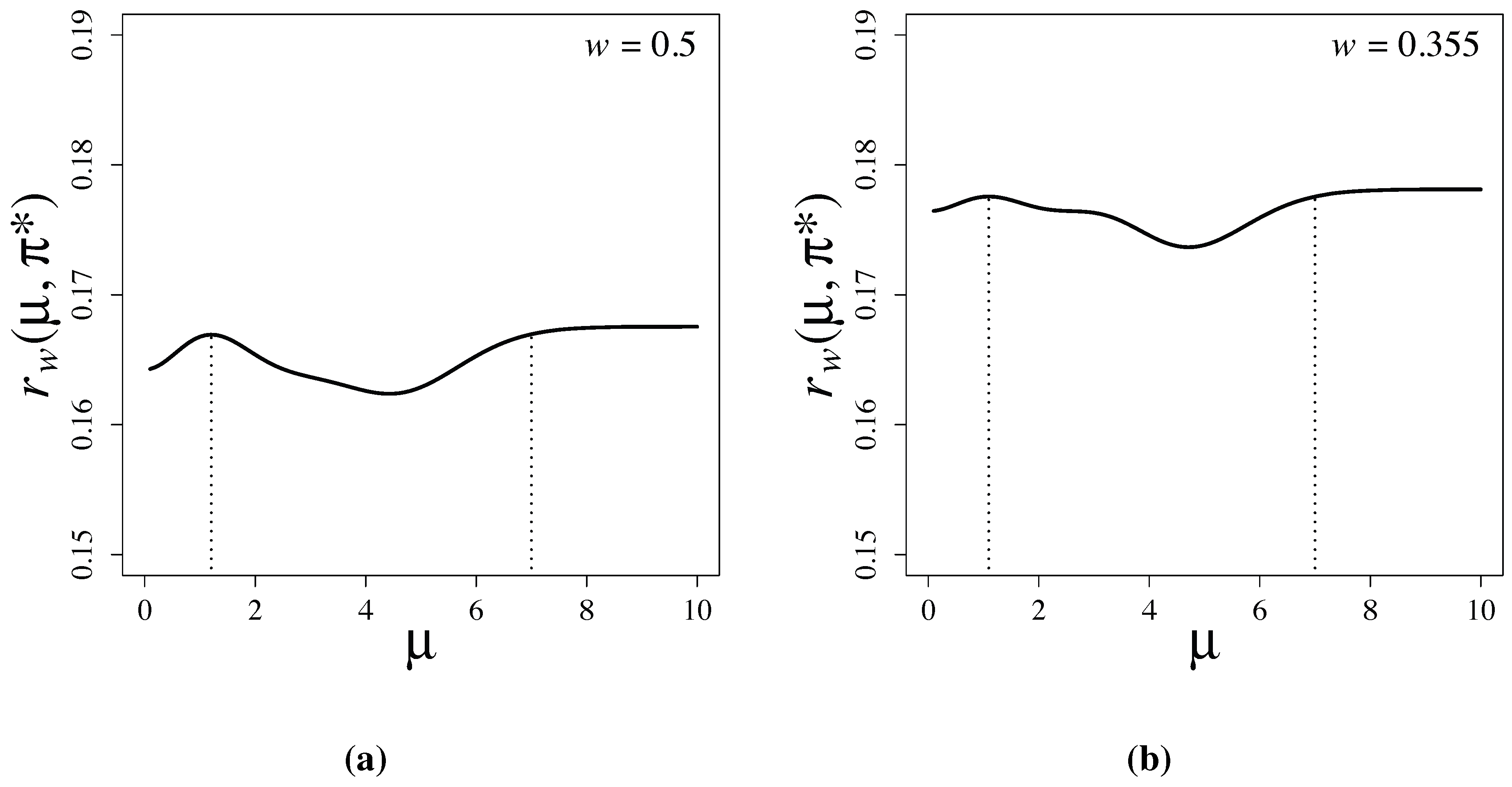
Figure 1 shows the numerically-obtained latent information priors. The priors have the form:
The parameter values are
,
and
, when
, and
,
and
, when
.
Lemma 2 below gives the risk of Bayesian testing based on the prior in Equation (18).
Lemma 2. Let:where and . Then, the risk in Equation (8) is given by:and the conditional mutual information in Equation (
1)
is given by: The first and second terms in Equation (20) do not depend on π. The third term in Equation (20) does not depend on μ.
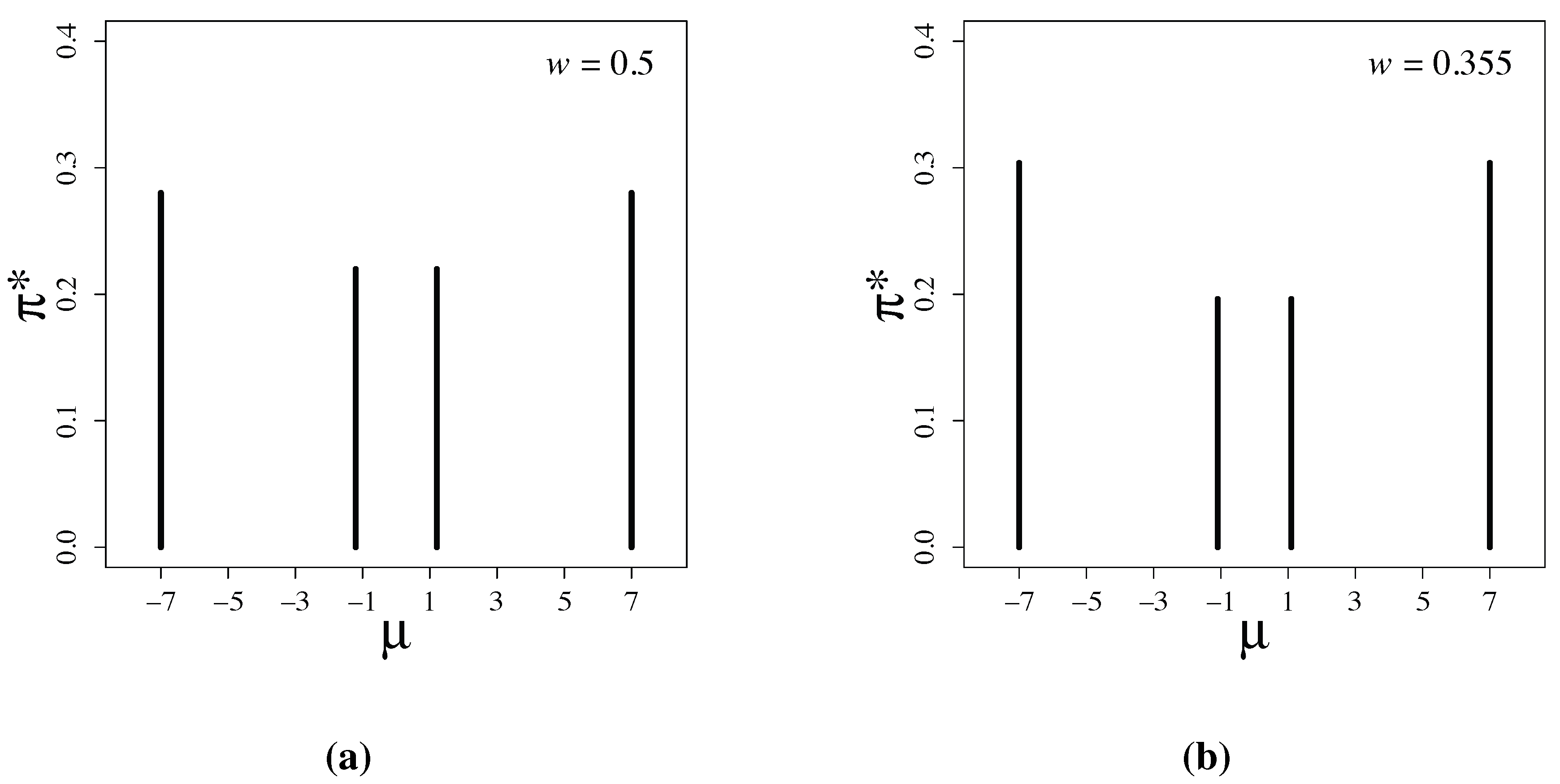
Figure 2 shows the risk functions of the latent information priors when
and
, respectively. Note that
is attained at
and
b in both examples. This is consistent with the proof of Theorem 1, and it is numerically verified that the prior maximizes the conditional mutual information. Furthermore, we observe that the supremum value,
, of the risk without restriction
is only slightly larger than the maximum value,
, with the restriction
. The risk functions rapidly converge as
μ exceeds seven.
Figure 2.
Risk functions of Bayesian testing based on latent information priors for (a) and for (b) . When , and . When , and . The vertical dotted lines indicate the locations of a and b.
Figure 2.
Risk functions of Bayesian testing based on latent information priors for (a) and for (b) . When , and . When , and . The vertical dotted lines indicate the locations of a and b.
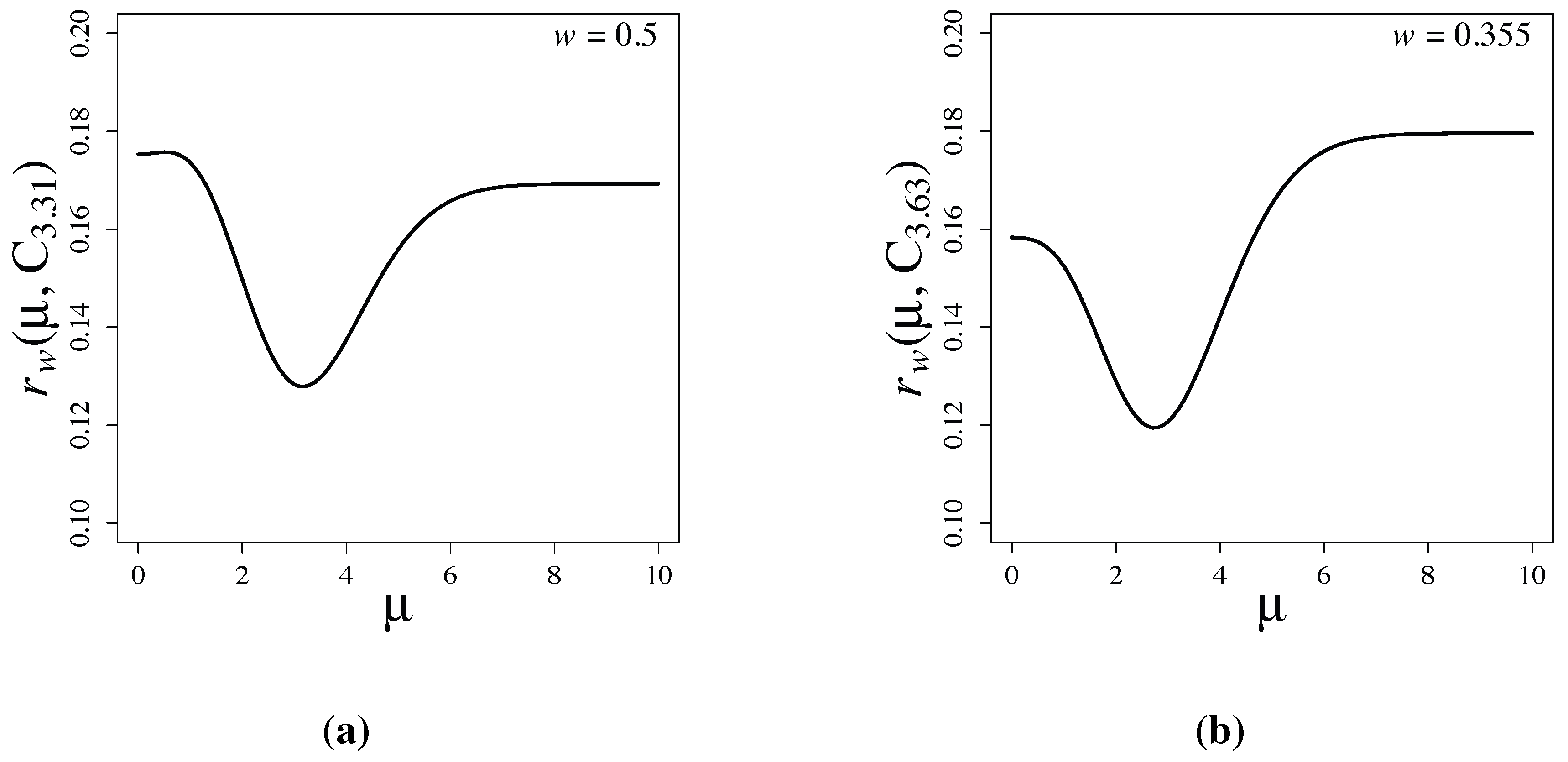
Since:
and
is small in our problem when
, the supremum value,
, of the risk function of the latent information prior,
, under the parameter restriction,
, is only slightly larger than the minimax value,
without the restriction. We see in the next section that the supremum,
, of the risk functions of commonly used priors are much larger than those of
.
The discreteness of latent information priors shown in
Figure 1 is a remarkable feature. In Bayesian statistics,
k-reference priors have been known to be discrete measures in many examples; see [
11,
12,
13]. The
k-reference prior is defined to be a prior maximizing the mutual information between
and
θ when we have a set,
, of
k-independent observations,
, from
in a parametric model,
. However, such discrete priors have not been widely used. Instead of
k-reference priors, reference priors introduced by Bernardo [
14] have been used for many problems. Reference priors are not discrete and are defined by considering the limit that the sample size
k goes to infinity. One main reason why discrete priors are not popular is that discrete priors are totally unacceptable form the viewpoint of subjective Bayes in which priors are considered to represent prior belief on parameters.
Although they have not been widely used, discrete priors, such as latent information priors, are reasonable from the viewpoint of prediction and objective Bayes. Various statistical problems, including estimation and testing, can be formulated from the viewpoint of prediction, and priors can be constructed by considering the conditional mutual information. Thus, latent information priors depending on the choice of variables to be predicted could play important roles in many statistical applications. Conditional mutual information is essential in information theory and naturally appeared in several studies in statistics; see e.g., [
15,
16]. Priors based on conditional mutual information and those based on unconditional mutual information are often quite different; see [
4].
Bayesian testing based on latent information priors is free from the Jeffreys-Lindley paradox [
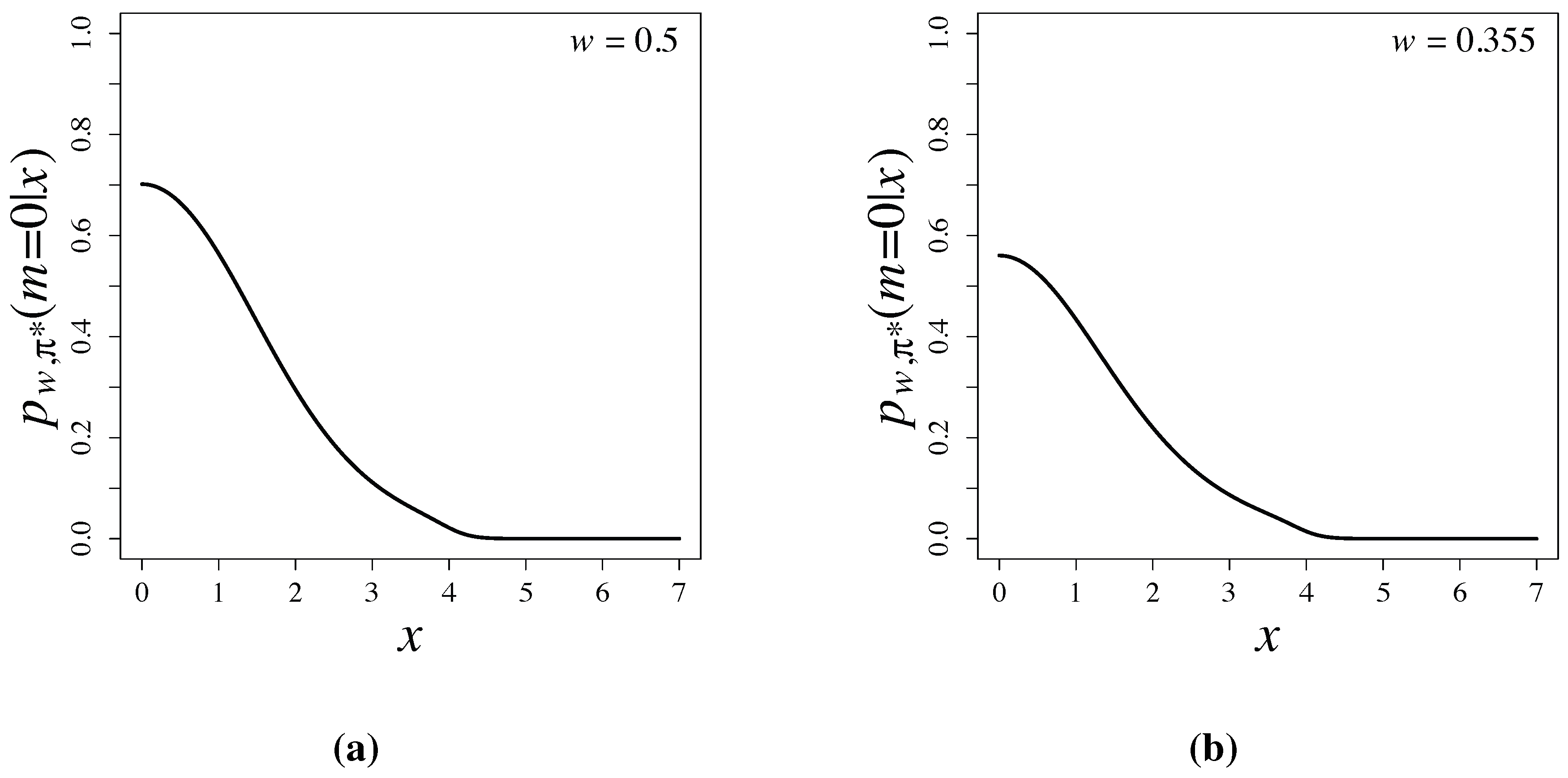
3], since the priors are constructed by using conditional mutual information and depend properly on sample sizes. Posterior probabilities,
, are shown in
Figure 3 and are compared with
p-values of the two-sided test in
Table 1. When
and 4, posterior probabilities are much smaller than
p-values of the two-sided test. Large differences of posterior probabilities and
p-values have been widely observed and discussed in [
1,
17,
18].
Figure 3.
Posterior probabilities based on latent information priors for (a) and for (b) .
Figure 3.
Posterior probabilities based on latent information priors for (a) and for (b) .
Table 1.
Comparison of posterior probabilities and p-values.
Table 1.
Comparison of posterior probabilities and p-values.
| x | 0 | 1 | 2 | 3 | 4 |
|---|
| 0.702 | 0.564 | 0.295 | 0.112 | 0.0217 |
| 0.560 | 0.434 | 0.220 | 0.0867 | 0.0145 |
| p-value (two-sided test) | 1 | 0.317 | 0.0455 | 0.00267 | |


