Abstract
When we try to make the best estimate of some quantity, the problem of combining results from different experiments is encountered. In multi-sensor data fusion, the problem is seen as combining observations provided by different sensors. Sensors provide observations and information on an unknown quantity, which can differ in precision. We propose a combined estimate that uses prior information. We consider the simpler aspects of the problem, so that two sensors provide an observation of the same quantity. The standard error of the observations is supposed to be known. The prior information is an interval that bounds the parameter of the estimate. We derive the proposed combined estimate methodology, and we show its efficiency in the minimum mean square sense. The proposed combined estimate is assessed using synthetic data, and an application is presented.
1. Introduction
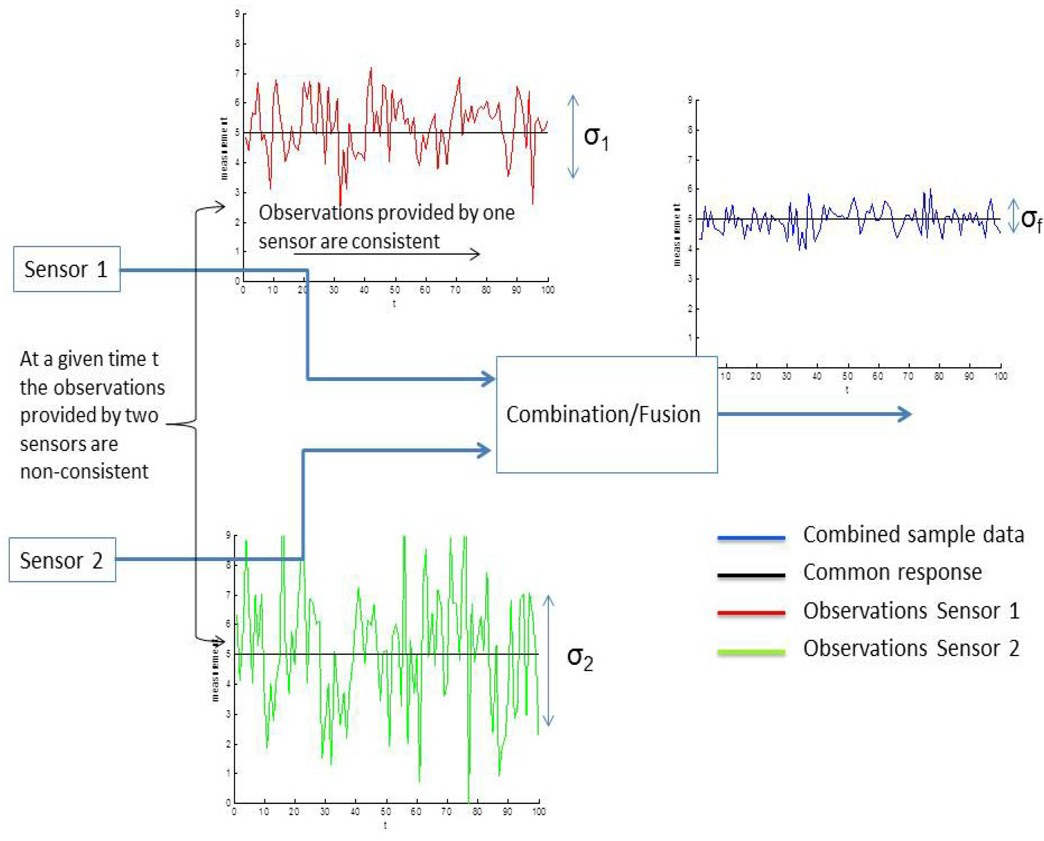
The problem of making a combined estimate as a weighted mean with weights inversely proportional to the variance was discussed previously in [1]. Research in this area is conducted to derive a combined estimate when the observations are partially consistent. For example, suppose two or more sensors perform; these sensors are used to provide observations on a common response variable. The sensors measure the same parameter, but their measurements differ in precision. The observations are partially consistent, because the observations obtained with the same sensor are assumed to be consistent and the observations provided by different sensors are assumed to be non-consistent. We present in Figure 1 the case of two sensors. To make inferences about the common parameter, we wish to make use of the combined sample data. These sensors are assumed to have no systematic biases, but to differ in precision. This is the case, for example, of the Global Navigation Satellite System (GNSS) application, where the same position can be observed with signals broadcast on different frequency bands and signals broadcast by different satellite systems. Heteroscedasticity is the key feature of the combined sample data. Research in this domain focuses on the joint definition of weights and combined estimators. In [2], the efficiency of the weighted mean with estimate variances was studied. The variance of the weighted regression was derived in [3]. A new estimator that is more efficient than the maximum likelihood estimate was developed in [4]. Further references and proposed estimators can be found in [5,6].

Figure 1.
Heteroscedasticity framework in information fusion.
Figure 1.
Heteroscedasticity framework in information fusion.
Most of the multi-sensors data fusion systems assume that the variances of processes are known (or estimated on the processes, but the error of estimation is not taken into account in the definition of the weights), and the classical Bayesian estimation is used to design fusion operators. When the measurements are independent, the least square (LS) estimate and the maximum likelihood (ML) estimate are the same. This classical fusion operator is the weighted mean with weights inversely proportional to the variance [7]. For dependent or correlated measurements, the weights are defined by the variances and covariance of the observations. They are a solution of a set of linear equations that link the variance of the fusion operator to the variances and covariance of the measures [8]. Unfortunately, in practice, the covariance is difficult to estimate, and few applications use the optimal fusion operator in this case [9].
Maximum a posteriori (MAP) estimators use in their implementation prior information to estimate a quantity. The Bayesian modeling of a problem allows one to integrate prior information on the data to fuse [10]. The a posteriori distribution that models the problem is defined by the product of a priori law with the likelihood distribution of the multi-sensor data. The prior information can be a priori law on the parameter to estimate [11,12] or on the mutual behavior of processes [13,14]. In the sequential Bayesian inference framework, the prior law models the information brought by the dynamic state equation of the Bayesian filter [15,16]. In all those cases, the fusion operator that merges the prior information with the observations is a weighted sum.
Some multi-sensor data fusion systems defined in the sequential Bayesian inference framework have to combine distributed estimates. Let us consider an estimate of the same state provided by different filters working in parallel. This is the case of filters having different observations provided by sensors of different kinds. It is shown in [17] that for two Kalman filters working in parallel, the process noise brings a correlation between the estimate states. The Track-to-Track fusion filter proposed by [17] uses a weighted sum to fuse the correlate estimate. The weights are, in this case, the function of the variances and covariance of the estimate state. In the proposed filter, a recursive expression of the estimate state covariance is derived in order to compute the weighted sum. Many different implementations of the Track-to-Track fusion filter can be found in published works [18]. The extension of the fusion technique to N filters in parallel was proposed by [19], but the filter is difficult to process in practice. Finally, a sub-optimal version of the filter proposed in [8] allows one to solve the problem of covariance estimation and to provide an easy solution to implement with good accuracy.
In the present paper, we consider a simple aspect of the problem, two sensors, , and observations, , distributed according to a Gaussian distribution of mean, m, and variance, . We propose a non-linear estimate that uses prior information in order to combine the observations. This information is an approximate value of m, assumed to be distributed according to a Gaussian law of variance, . Furthermore, m is assumed to be inside the interval, . It is shown in [10] that the classical (MAP) estimate is a weighted sum of the observations and of the prior information. We show that the proposed fusion operator outperforms the MAP estimate in the minimum quadratic error sense. The proposed fusion operator is assessed for a multi-sensor system that estimates the position of an object. The multi-sensor system is composed of a multi-band GNSS receiver, a yaw rate sensor and a speed meter sensor. In this case, the data fusion system has to combine the estimated position obtained for each band of the GNSS receiver. The measurements of direction and velocity provided by the dead reckoning sensors are the prior information on the parameter to estimate.
2. Problem Statement
Let us consider and , two random variables, and and , their realizations at instant, k. We consider the case of two sensors providing two measures, and . The random variables, and , are assumed to be independent with the same mean, m, and distributed according to Gaussian law, and . The variance of these random variables are, respectively, and . The maximum-likelihood estimation (MLE) fusion operator is the following weighted sum:
The MAP fusion operator is the following weighted sum:
where is the imprecise prior information assumed to be distributed according to a Gaussian law, , of variance, , and mean, m. The fused measurement at instant k is , the realization of the random variable . The weights are defined as follows:
We can distinguish two kinds of realizations of the random variable pair, :
- Realizations situated on both sides of the mean, m, such as and or and .
- Realizations situated on the same side of the mean, m, such as and or and .
3. Non-Linear Fusion Operator
3.1. The Non-Linear Transformation
3.1.1. Definition of the Non-Linear Transformation
Let be the non-linear fusion (NLF) of and . We propose to define the non-linear MAP fusion operator, for , as follows:
where the weights are defined with Equation (3). The non-linear fusion operator is biased. The upper and lower bound are indeed not necessarily centered on the mean value, m. The mean square error (MSE) takes into account the variance and bias of an estimator. We derive in the next paragraph a condition on the proposed non-linear transformation that guarantees a smaller MSE for the proposed operator.
- If and
- If and
- otherwise and or and
3.1.2. A Condition on the Non-Linear Transformation
Let us define the following notation for the fused measurements:
where the coefficients of normalization, P and N, are defined as follows:
- If and or and , we notice , , the respective MSE of the non-linear fusion operator output and of the linear fusion operator output.
- otherwise, we notice , , the respective MSE for the non-linear fusion operator and for the linear fusion operator.
We show in Appendix 2 that the quadratic error, , will be smaller than the quadratic error, , if the following inequality holds:
The terms of this equation are defined by:
Term 1:
Term 2:
Term 3:
Term 4:
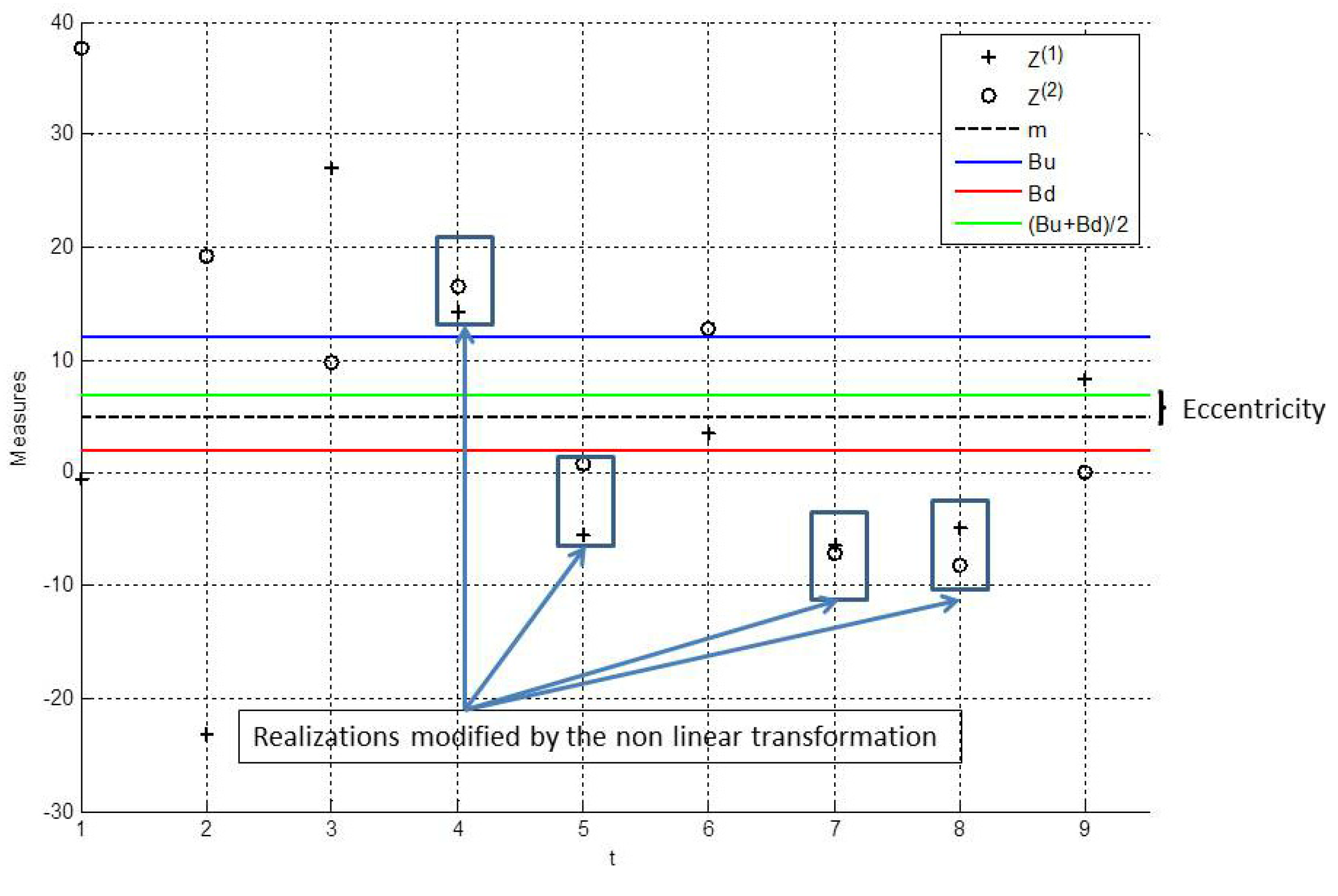
where in the Terms 1–4, the difference between the integrals are due to the signs of , as defined in Equations (4) and (5).The condition of Equation (10) depends on the variance of the fused random variables, on the interval size and on its eccentricity, . We show in Figure 2 several realizations of and , an interval and its associated eccentricity. We show in this figure the realizations that will be modified by the non-linear transformation, the observations that satisfy the conditions: or . In the next paragraph, we propose a function, , that holds the inequality in Equation (10) for an interval that contains the parameter for estimating.

Figure 2.
Example of non-linear transformation.
Figure 2.
Example of non-linear transformation.
3.2. Transformation Function
3.2.1. Conditions on the Transformation Function
The function, , is defined heuristically. In the centered case, , we can define two conditions to hold the inequality in Equation (10):
- Condition 1:
- Condition 2:
These two conditions are verified for a positive function of the difference between two measurements, . For and , the function, , is indeed centered and symmetric. The Terms 1 and 4 are null in this case. Furthermore, if the function, , is positive, the Terms 2 and 3 are negative, and the inequality in Equation (10) is negative. In the next paragraph, we propose a non-linear function that matches these conditions, and we show, in the experimentation, that the inequality in Equation (10) for this function is always negative, even if the interval is not centered on the parameter to be estimated.
3.2.2. Definition of the Transformation Function
The principle of the non-linear transformation is to, respectively, add or subtract a positive offset, , if or . Let us consider the following statistic distributions:
with:
Let us define the following relation:
then, we can derive the following expression for d:
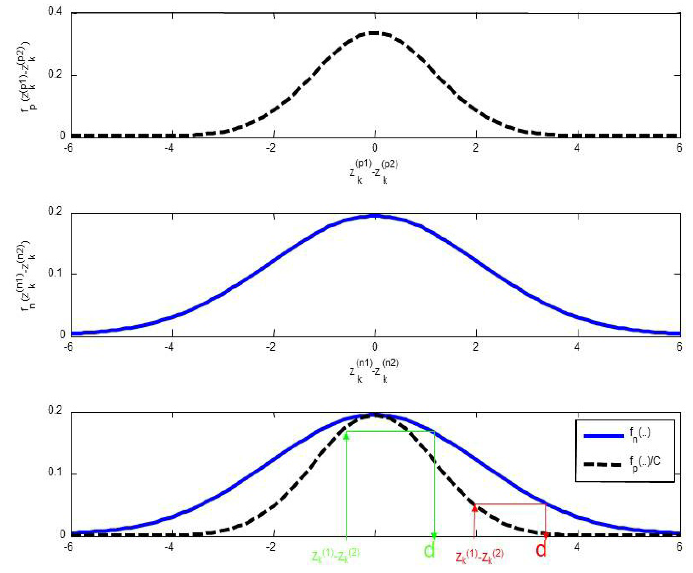
We explain in Figure 3 the principle of the definition of d. The experimentation presented in the next paragraph shows that the proposed non-linear function holds the inequality in Equation (10). We assess in this experimentation the proposed fusion operator on synthetic data.
- Let be the Gaussian distribution of the difference between the random variables, and . This distribution is a zero-mean, and its variance is given by .
- Let be the Gaussian distribution of the difference between the random variables, and . This distribution is a zero-mean, and its variance is given by .

Figure 3.
Principle of the non-linear function.
Figure 3.
Principle of the non-linear function.
4. Experimentation
In this experimentation, we first verify the inequality in Equation (10) for the proposed non-linear function. The fusion operator is assessed in a second experimentation, and finally, we demonstrate the feasibility of the proposed operator, in a third experimentation, for the fusion of data provided by a multi-sensor system.
4.1. Verification of the Inequality
In order to show that the proposed non-linear fusion operator has an output MSE lower than the classical linear fusion operator, we compute the left term of inequality in Equation (10). This term is defined as a constraint on the non-linear function and is equal to . The evaluation of this constraint is processed by numerical integration of Terms 1–4 defined in paragraph 3.1.2. We show that the proposed non-linear function holds the inequality in Equation (10), because the constraint is negative or null for all interval sizes and eccentricity.
We show in Figure 4 the constraint as a function of the interval length, , and of the eccentricity, . The curves of Figure 4 are obtained for and . When , the fusion is less accurate, because the random variable, , brings little information on the parameter to estimate (so ). In this case, the constraint is close to zero, so the proposed and the MAP fusion operator are similar. When , the constraint is negative for all the intervals and values of eccentricity. We can notice that for small values of the interval size, the constraint is close to zero. In this case, , because the prior information is very accurate, and the fusions operators do not use the observations. In conclusion, the greatest is the difference between the variances of and ; less interesting is the fusion. We can notice that this conclusion is also valid for the classical fusion operator. However, the constraint is always negative, and it shows that the proposed fusion operator is more accurate than the classical MAP fusion operator.
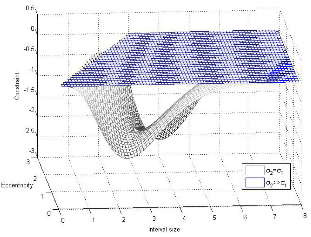
Figure 4.
The constraint as a function of the interval and eccentricity.
Figure 4.
The constraint as a function of the interval and eccentricity.

We show in Figure 5 the normalized value of the constraint, , as a function of the interval size and of the eccentricity. The constraint is processed for two values of and the normalization allows one to compare these two cases. We can observe in Figure 5 that when the interval length and the eccentricity increase for , the constraint tends towards zero more quickly than for . The probability of and to be in a given interval is indeed higher for than for . When this probability decreases, less observations are modified by the non-linear transformation, and the output variance of the non-linear fusion operator tends to the output variance of the MAP fusion operator.
We show in this experimentation that from a theoretical point of view, the proposed fusion operator is more accurate than the classical fusion operator, because the proposed non-linear function holds the inequality in Equation (10). In the next paragraph, we assess the proposed operator with synthetic data.
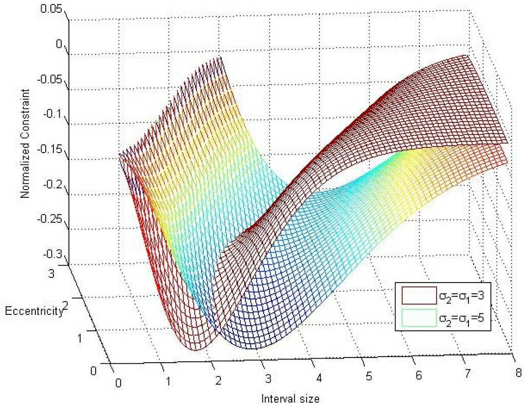
Figure 5.
The constraint for two values of .
Figure 5.
The constraint for two values of .

4.2. Assessment of the Fusion Operator
In this experimentation, we compare the non-linear fusion operator with the classical ML and MAP fusion operators. We consider a constant signal of samples. We show in Figure 6a a temporal series of . The prior information is an interval represented on this figure by two horizontals dotted lines.
To compare the operators, we estimate the MSE between the fused measurements and the parameters to be estimated. For the ML fusion operator, the MSE is equal to the variance, because the combined estimate is unbiased. We report in Table 1 the parameters of the signals and the theoretical output variance of the classical ML fusion operator.
In order to assess the MAP and the non-linear fusion operator, we process 1,000 realizations of the temporal series, and . For each experiment, we randomly generate the prior information, , according to a Gaussian distribution of mean m and variance . We report in Table 2 and we show in Figure 6b the MSE of the MAP and nonlinear fusion operator as a function of .
We notice in Figure 6b and in Table 2 that the MSE of the proposed non-linear fusion operator is always inferior or equal to the MSE of the MAP and LS fusion operators. When is small, the prior information is accurate and tends to one. The MSE of the MAP estimate and of the non-linear fusion operator tends to zero. In this case, the MAP estimate tends to be the same as the non-linear fusion operator, because and tend to zero. When is large, the prior information is inaccurate. The MSE of the MAP estimate and of the non-linear fusion operator tends to the MSE of the LS estimate. The three fusion operators tend to be identical, because is close to zero, and the interval length Bu-Bd is large. Then, no transformation is processed by the non-linear fusion operator.
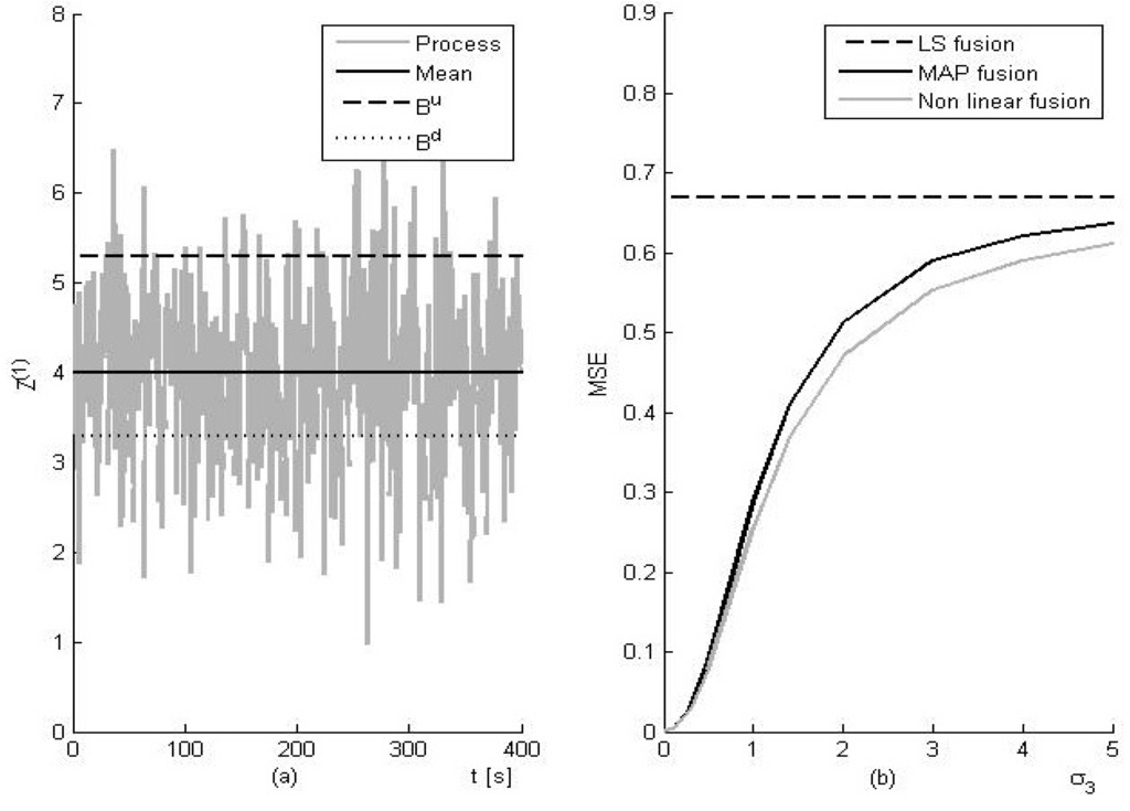
Figure 6.
Example of process and mean standard error (MSE) of the proposed operator.
Figure 6.
Example of process and mean standard error (MSE) of the proposed operator.


Table 1.
Theoretical parameters of the signals.
| Mean | MSE | |
|---|---|---|
| First signal | 4 | 1 |
| Second signal | 4 | 2 |
| Linear fusion | 4 | 0.666 |
The only difference between the MAP and the non-linear fusion operators is the observation weighted by . In the non-linear fusion case, this observation is processed with a nonlinear function in order to decrease the correlation between and . Therefore, this transformation decreases the MSE of the fusion operator compared to the MSE of the MAP estimate. We notice in Figure 6b that for , the difference between the MSE increases when increases, so, when increases ( decreases because the prior information is less accurate). However, for , the number of transformations processed by the non-linear transformation decreases, and the difference between the MSE decreases.

Table 2.
MSE of the NL (non-linear) and Maximum a posteriori (MAP) fusion operators.
| Prior information | Mean Square Error | |
|---|---|---|
| Accuracy σ3 | MAP Fusion | NL Fusion |
| 0.0 | 0.0000 | 0.0000 |
| 0.1 | 0.0030 | 0.0030 |
| 0.3 | 0.0294 | 0.0274 |
| 0.5 | 0.0876 | 0.0779 |
| 1.0 | 0.2884 | 0.2566 |
| 1.4 | 0.4106 | 0.3695 |
| 2.0 | 0.5135 | 0.4711 |
| 3.0 | 0.5902 | 0.5534 |
| 4.0 | 0.6218 | 0.5909 |
| 5.0 | 0.6369 | 0.6114 |
4.3. Multi-Sensor Estimation
In this experimentation, we want to assess a multi-sensor fusion system that uses the proposed non-linear transformation. The system, embarked on a vehicle, is composed of a multi-band GNSS receiver, a speedometer and a magnetometer.
The multi-bands GNSS receiver provides measurements of positions obtained in the GNSS L1 band and in the GNSS L2C band. The measurement rate is equal to 10 Hz, and we assume a standard positioning service, non-differential horizontal (latitude & longitude) positioning and SAoff. The classical receiver at the L1 band, simulated in this experimentation, has a four meter root means square (RMS) error (the error is the distance between the position and its estimate). For a measurement rate of 10 Hz, the estimate position is the averaging of 100 observations for the L1 band and five observations for the L2C band. A receiver can indeed compute a position every millisecond at the L1 band and every 20 milliseconds at the L2C band. If the horizontal latitude and longitude errors were not correlated, the RMS error would be inversely proportional to the square root of the number of measurements. However, the errors are correlated, and this causes the error from averaging to decrease at a slower rate than if the errors were not correlated. It is a reasonable assumption to consider a double RMS error for the L2C band. A speedometer is installed in a vehicle. The uncertainty of the speedometer is equal to 5% of the vehicle speed. In this context, we assume a bias of 5% and an additive Gaussian noise on the measurements. The noise variance is equal to m/s. Finally, we assume an additive Gaussian noise on the measurements of direction. The noise variance is equal to two degrees.
The plots in Figure 7 show the trajectory and the sensors’ measurements. In Figure 7, the left figure shows the trajectory and the observed positions provided by the GNSS receiver. In Figure 7, the top right figure presents the measurements of direction provided by the magnetometer and the filtered directions obtained with a circular filter [20]. The bottom right figure presents the measurements of speed, and , along the x- and y-axis. These measurements are the projections of the velocity vectors processed with the observed noisy direction and speed (vector magnitude).
In our implementation, the upper and lower bound intervals of the proposed non-linear transformation are defined at time, , with direction and speed. The non-linear transformation is applied to each component, x, y, of the position. For the x component, the interval center is the estimated x component at t plus the variation in position during along the x-axis (*). The size of the interval is fixed to ; this value is fixed in practice. The same method is used for the non-linear fusion of the component, y.
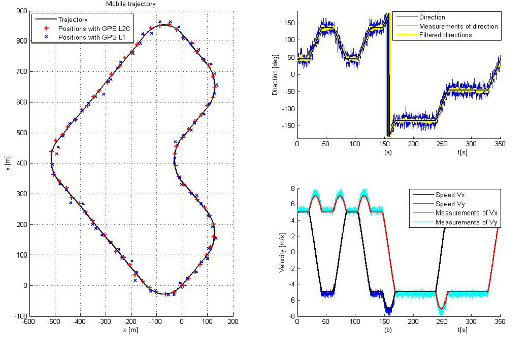
Figure 7.
Trajectory and sensors’ measurements.
Figure 7.
Trajectory and sensors’ measurements.

We report in Table 3 the mean square error of the position for the x and y directions and the position RMS error. We report this statistical parameter for the proposed non-linear fusion method, the ML and MAP fusion operators and for the GPS L1 positions.

Table 3.
Error of position.
| Statistical parameter | MSE x | MSE y | RMS error |
|---|---|---|---|
| GPS L1 | 2.0549 | 2.0141 | 2.0169 |
| ML fusion | 1.3565 | 1.4039 | 1.6612 |
| MAP fusion | 0.2524 | 0.2556 | 0.7128 |
| non-linear fusion | 0.2350 | 0.2365 | 0.6867 |
This experimentation shows a possible application of the proposed combined estimate. The previous estimate with the measurements of displacement (provided by the dead reckoning sensors) are used to construct the prior information (lower and upper bound of the interval). In this case, the eccentricity is distributed according to a Gaussian law. As shown in the previous paragraph, the MSE of the proposed combined estimate is lower than the classical fusion operators. However, the difference between the MSE of the MAP estimate and of the non-linear fusion operator is not as high as the one obtained in the assessment of the fusion operators. For this practical case, the true position is some time not contained in the interval defined by the upper and lower bound, and the non-linear transformation has an additive bias that increases the MSE. This is the principal limitation of the proposed fusion operator.
The limitation of the non-linear fusion operator is due to the definition of an interval that contains the parameter to be estimated. If the interval is small, the probability to be outside this interval is high, and the MSE of the proposed method can be superior to the MSE of the MAP estimate. If the interval is large, the proposed estimate has little interest, because its MSE is close to the MSE of the LS estimate. Therefore, there is an ambivalence between these two cases, and the size of the interval must be, in practice, tuned by the user in order to improve the estimation.
5. Conclusions
In this article, we propose a new combined estimate that uses a prior law. The proposed new method combines observations provided by two sensors. The prior law is an interval that contains the quantity to estimate. The proposed fusion operator is more accurate in the minimum mean square sense than the classical ML and MAP fusion operators.
The proposed combined estimate is based on a non-linear transformation of the signals. The aim of this transformation is to decrease the covariance between the observations in order to decrease the output mean square error of the fusion operator. We define a condition for a non-linear transformation to decrease the covariance. We derive the function and the associated non-linear transformation that holds this condition.
As expected from the theoretical derivation provided in the article, we show in the experimentation that the proposed non-linear combined estimate outperforms the classical fusion operator when the quantity to be estimated is in the interval. We propose an example of a practical implementation of the proposed combined estimate. We show that the non-linear fusion improves the positioning of a multi-sensor system composed of a multi-band GNSS receiver and dead reckoning sensors.
The prospect of this work concerns the extension of the proposed method to more than two observations.
Conflict of Interest
The authors declare no conflict of interest.
References
- Cochran, W.G. Problem arising in the analysis of a series of similar experiments. J. R. Stat. Soc. 1937, 4, 102–118. [Google Scholar] [CrossRef]
- Cochran, W.G.; Carroll, S.P. A sampling investigation of the efficiency of weighting inversely as the estimated variance. Biometrics 1953, 9, 447–459. [Google Scholar] [CrossRef]
- Bement, T.R.; Williams, J.S. Variance of weighted regression estimators when sampling errors are independent and heteroscedastic. J. Am. Stat. Assoc. 1969, 64, 1369–1382. [Google Scholar] [CrossRef]
- Neyman, J.; Scott, E. Consistent estimators based on partially consistent observations. Econometrica 1948, 16, 1–32. [Google Scholar] [CrossRef]
- Rao, J.N.K. Estimating the common mean of possibly different normal populations: A simulation study. J. Am. Stat. Assoc. 1980, 75, 447–453. [Google Scholar] [CrossRef]
- Tsao, M.; Wu, C. Empirical likelihood inference for a common mean in the presence of heteroscedasticity. Can. J. Stat. 2006, 34, 45–59. [Google Scholar] [CrossRef]
- Gustafsson, F. Adaptative Filtering and Change Detection; Wiley: New York, NY, USA, 2001. [Google Scholar]
- Shin, V.; Lee, Y.; Choi, T.S. Generalized Millman’s formula and its application for estimation problems. Signal Process. 2006, 86, 257–266. [Google Scholar] [CrossRef]
- Kacemi, J.; Reboul, S.; Benjelloun, M. Information Fusion in a Multi-Frequencies GPS Receiver. In Proceedings of the IEEE International Conference on Aerospace And Electronics Systems Society (IEEE, AESS), Position Location and Navigation Symposium (PLANS), Monterey, CA, USA, 26–29 April 2004; pp. 399–404.
- Lavielle, M.; Lebarbier, E. An application of MCMC methods for the multiple change-points problem. Signal Process. 2001, 81, 39–53. [Google Scholar] [CrossRef]
- Robert, C.P. The Bayesian Choice, 2nd ed.; Springer: New York, NY, USA, 2001. [Google Scholar]
- Stienne, G.; Reboul, S.; Azmani, M.; Boutoille, S.; Choquel, J.B.; Benjelloun, M. Bayesian change-points estimation applied to GPS signal tracking. ISRN Signal Process. 2011. [Google Scholar] [CrossRef]
- Boutoille, S.; Reboul, S.; Benjelloun, M. A hybrid fusion system applied to off-line detection and change-points estimation. Inf. Fusion 2010, 11, 325–337. [Google Scholar] [CrossRef]
- Reboul, S.; Benjelloun, M. Joint segmentation of the wind speed and direction. Signal Process. 2006, 86, 744–759. [Google Scholar] [CrossRef]
- Mitchell, H.B. Multi-Sensor Data Fusion, An Introduction; Springer: Berlin/Heidelberg, Germany, 2007. [Google Scholar]
- Zhu, Y.; You, Z.; Zhao, J.; Zhang, K.; Li, X.R. The optimality for the distributed kalman filtering fusion with feedback. Automatica 2001, 37, 1489–1493. [Google Scholar] [CrossRef]
- Bar-Shalom, Y.; Campo, L. The effect of the common process noise on the two-sensor fused-track covariance. IEEE Trans. Aerosp. Electron. Syst. 1986, 22, 803–805. [Google Scholar] [CrossRef]
- Gao, J.B.; Harris, C.J. Some remarks on kalman filters for the multisensor fusion. Inf. Fusion 2002, 3, 191–201. [Google Scholar] [CrossRef]
- Chen, H.; Kirubarajan, T.; Bar-Shalom, Y. Performance limits of track-to-track fusion vs. centralized estimation: Theory and application. IEEE Trans. Aerosp. Electron. Syst. 2003, 39, 386–400. [Google Scholar] [CrossRef]
- Azmani, M.; Reboul, S.; Choquel, J.-B.; Benjelloun, M. A Recursive Fusion Filter for Angular Data. In Proceedings of the IEEE International Conference on Robotics and Biomimetics, Guilin, China, 19–23 December 2009; pp. 882–887.
Appendix 1
In this appendix, we show that the realizations of two random variables on the same side of the mean are positively correlated. We show that the realizations on both sides are negatively correlated. Let be the distribution of the random variables, and . The covariance of and is given by:
We develop the covariance Equation (13) for the different kind of realizations of and . It follows that:
with:
is a term associated with the realizations of and , and is a term associated with the realizations of and . Let be the covariance of , and be the covariance of , . These covariances are given by the following expressions:
with:
It follows:
Furthermore, we state that:
It follows:
We can then define:
Finally, it follows:
According to the previous equation, the covariance of , is positive, and the covariance of , is negative.
Appendix 2
In this appendix, we derive the condition that the mean square error, , of the proposed non-linear fusion operator is lower than the mean square error, , of the linear fusion operator. This error is lower if we decrease the covariance between the realizations of the processes that correlated positively, because . The mean square errors, and , of the fusion operators are given by:
With:
It follows:
Then, is lower than , if the following condition holds:
© 2013 by the authors; licensee MDPI, Basel, Switzerland. This article is an open access article distributed under the terms and conditions of the Creative Commons Attribution license (http://creativecommons.org/licenses/by/3.0/).
