Abstract
Information-theoretic quantities, such as entropy and mutual information (MI), can be used to quantify the amount of information needed to describe a dataset or the information shared between two datasets. In the case of a dynamical system, the behavior of the relevant variables can be tightly coupled, such that information about one variable at a given instance in time may provide information about other variables at later instances in time. This is often viewed as a flow of information, and tracking such a flow can reveal relationships among the system variables. Since the MI is a symmetric quantity; an asymmetric quantity, called Transfer Entropy (TE), has been proposed to estimate the directionality of the coupling. However, accurate estimation of entropy-based measures is notoriously difficult. Every method has its own free tuning parameter(s) and there is no consensus on an optimal way of estimating the TE from a dataset. We propose a new methodology to estimate TE and apply a set of methods together as an accuracy cross-check to provide a reliable mathematical tool for any given data set. We demonstrate both the variability in TE estimation across techniques as well as the benefits of the proposed methodology to reliably estimate the directionality of coupling among variables.
1. Introduction
Complex dynamical systems consisting of nonlinearly coupled subsystems can be found in many application areas ranging from biomedicine [1] to engineering [2,3]. Teasing apart the subsystems and identifying and characterizing their interactions from observations of the system’s behavior can be extremely difficult depending on the magnitude and nature of the coupling and the number of variables involved. In fact, the identification of a subsystem can be an ill-posed problem since the definition of strong or weak coupling is necessarily subjective.
The direction of the coupling between two variables is often thought of in terms of one variable driving another so that the values of one variable at a given time influence the future values of the other. This is a simplistic view based in part on our predilection for linear or “intuitively understandable” systems. In nonlinear systems, there may be mutual coupling across a range of temporal and spatial scales so that it is impossible to describe one variable as driving another without specifying the temporal and spatial scale to be considered.
Even in situations where one can unambiguously describe one variable as driving another, inferring the actual nature of the coupling between two variables from data can still be misleading since co-varying variables could reflect either a situation involving coupling where one variable drives another with a time delay or a situation where both variables are driven by an unknown third variable each with different time delays. While co-relation (we use the term co-relation to describe the situation where there is a relationship between the dynamics of the two variables; this is to be distinguished from correlation, which technically refers only to a second-order statistical relationship) cannot imply causality [4], one cannot have causality without co-relation. Thus co-relation can serve as a useful index for a potential causal interaction.
However, if past values of one variable enable one to predict future values of another variable, then this can be extremely useful despite the fact that the relationship may not be strictly causal. The majority of tests to identify and quantify co-relation depend on statistical tests that quantify the amount of information that one variable provides about another. The most common of these are based on linear techniques, which rely exclusively on second-order statistics, such as correlation analysis and Principal Component Analysis (PCA), which is called Empirical Orthogonal Functions (EOFs) in geophysical studies [5]. However, these techniques are insensitive to higher-order nonlinear interactions, which can dominate the behavior of a complex coupled dynamical system. In addition, such linear methods are generally applied by normalizing the data, which implies that they do not depend on scaling effects.
Information-theoretic techniques rely on directly estimating the amount of information contained in a dataset and, as such, rely not only on second-order statistics, but also on statistics of higher orders [6]. Perhaps most familiar is the Mutual Information (MI), which quantifies the amount of information that one variable provides about another variable. Thus MI can quantify the degree to which two variables co-relate. However, since it is a symmetric measure MI cannot distinguish potential directionality, or causality, of the coupling between variables [7].
The problem of finding a measure that is sensitive to the directionality of the flow of information has been widely explored. Granger Causality [8] was introduced to quantify directional coupling between variables. However, it is based on second-order statistics, and as such, it focuses on correlation, which constrains its relevance to linear systems. For this reason, generalizations to quantify nonlinear interactions between bi-variate time-series have been studied [9]. Schreiber proposed an information-theoretic measure called Transfer Entropy (TE) [7], which can be used to detect the directionality of the flow of information. Transfer Entropy, along with other information-based approaches, is included in the survey paper by Hlavackova-Schindler et al. [10] and differentiation between the information transfer and causal effects are discussed by Lizier and Propenko [11]. Kleeman presented both TE and time-lagged MI as applied to ensemble weather prediction [12]. In [13], Liang explored the information flow in dynamical systems that can be modeled by equations obtained by the underlying physical concepts. In such cases, the information flow has been analyzed by the evolution of the joint probability distributions using the Liouville equations and by the Fokker-Planck equations, in the cases of the deterministic and stochastic systems, respectively [13].
TE has been applied in many areas of science and engineering, such as neuroscience [1,14], structural engineering [2,3], complex dynamical systems [15,16] and environmental engineering [17,18]. In each of these cases, different approaches were used to estimate TE from the respective datasets. TE essentially quantifies the degree to which past information from one variable provides information about future values of the other variable based solely on the data without assuming any model regarding the dynamical relation of the variables or the subsystems. In this sense TE is a non-parametric method. The dependency of the current sample of a time series on its past values is formulated by kth and lth order Markov processes in Schreiber [7] to emphasize the fact that the current sample depends only on its k past values and the other process’s past l values. There also exist parametric approaches where the spatio-temporal evolution of the dynamical system is explicitly modeled [15,16]. However, in many applications it is precisely this model that we would like to infer from the data. For this reason, we will focus on non-parametric methods.
Kaiser and Schreiber [19], Knuth et al. [20], and Ruddell and Kumar [17,18] have expressed the TE as a sum of Shannon entropies [21]. In [17,18], individual entropy terms were estimated from the data using histograms with bin numbers chosen using a graphical method. However, as we discuss in Appendix AI, TE estimates are sensitive to the number of bins used to form the histogram. Unfortunately, it is not clear how to optimally select the number of bins in order to optimize the TE estimate.
In the literature, various techniques have been proposed to efficiently estimate information-theoretic quantities, such as the entropy and MI. Knuth [22] proposed a Bayesian approach, implemented in Matlab and Python and known as the Knuth method, to estimate the probability distributions using a piecewise constant model incorporating the optimal bin-width estimated from data. Wolpert and Wolf [23] provided a successful Bayesian approach to estimate the mean and the variance of entropy from data. Nemenman et al. [24] utilized a mixture of Dirichlet distributions-based prior in their Bayesian Nemenman, Shafee, and Bialek (NSB) entropy estimator. In another study, Kaiser and Schreiber [19] give different expressions for TE as a summation and subtraction of various (conditional/marginal/joint) Shannon entropies and MI terms. However, it has been pointed out that summation and subtraction of information-theoretic quantities can result in large biases [25,26]. Prichard and Theiler [25] discuss the “bias correction” formula proposed by Grassberger [27] and conclude that it is better to estimate MI utilizing a “correlation integral” method by performing a kernel density estimation (KDE) of the underlying probability density functions (pdfs). KDE tends to produce a smoother pdf estimate from data points as compared to its histogram counterpart. In this method, a preselected distribution of values around each data point is averaged to obtain an overall, smoother pdf in the data range. This preselected distribution of values within a certain range, which is known as a “kernel”, can be thought of as a window with a bandwidth [28]. Commonly-used examples of kernels include “Epanechnikov”, “Rectangular”, and “Gaussian” kernels. Prichard and Theiler showed that pdf models obtained by KDE can be utilized to estimate entropy [25] and other information theoretic quantities, such as the generalized entropy and the Time Lagged Mutual Information (TLMI), using the correlation integral and its approximation through the correlation sums [7]. In [25], Prichard and Theiler demonstrated that the utilization of correlation integrals corresponds to using a kernel that is far from optimal, also known as the “naïve estimator” described in [28]. It is also shown that the relationship between the correlation integral and information theoretic statistics allows defining “local” versions of many information theoretical quantities. Based on these concepts, Prichard and Theiler demonstrated the interactions among the components of a three-dimensional chaotic Lorenz model with a fractal nature [25]. The predictability of the dynamical systems, including the same Lorenz model have been explored by Kleeman in [29,30], where a practical approach for estimating entropy was developed for dynamical systems with non-integral information dimension.
In the estimation of information-theoretical quantities, the KDE approach requires estimation of an appropriate radius (aka bandwidth or rectangle kernel width) for the estimation of the correlation integral. In general cases, this can be accomplished by the Garassberger-Procaccia algorithm, as in [31–33]. In order to compute the TE from data using a KDE of the pdf, Sabesan and colleagues proposed a methodology to explore an appropriate region of radius values to be utilized in the estimation of the correlation sum [14].
The TE can be expressed as the difference between two relevant MI terms [19], which can be computed by several efficient MI estimation techniques using variable bin-width histograms. Fraser and Swinney [34] and Darbellay and Vajda [35] proposed adaptive partitioning of the observation space to estimate histograms with variable bin-widths thereby increasing the accuracy of MI estimation. However, problems can arise due to the subtraction of the two MI terms as described in [19] and explained in [25,26].
Another adaptive and more data efficient method was developed by Kraskov et al. [36] where MI estimations are based on k-nearest neighbor distances. This technique utilizes the estimation of smooth probability densities from the distances between each data sample point and its k-th nearest neighbor and as well as bias correction to estimate MI. It has been demonstrated [36] that no fine tuning of specific parameters is necessary unlike the case of the adaptive partitioning method of Darbellay and Vajda [35] and the efficiency of the method has been shown for Gaussian and three other non-Gaussian distributed data sets. Herrero et al. extended this technique to TE in [37] and this has been utilized in many applications where TE is estimated [38–40] due to its advantages.
We note that a majority of the proposed approaches to estimate TE rely on its specific parameter(s) that have to be selected prior to applying the procedure. However, there are no clear prescriptions available for picking these ad hoc parameter values, which may differ according to the specific application. Our main contribution is to synthesize three established techniques to be used together to perform TE estimation. With this composite approach, if one of the techniques does not agree with the others in terms of the direction of information flow between the variables, we can conclude that method-specific parameter values have been poorly chosen. Here, we propose using three methods to validate the conclusions drawn about the directions of the information flow between the variables, as we generally do not possess a priori facts about any physical phenomenon we explore.
In this paper, we propose an approach that employs efficient use of histogram based methods, adaptive partitioning technique of Darbellay and Vajda, and KDE based TE estimations, where fine tuning of parameters is required. We propose a Bayesian approach to estimate the width of the bins in a fixed bin-width histogram method to estimate the probability distributions from data.
In the rest of the paper, we focus on the demonstration of synthesizing three established techniques to be used together to perform TE estimation. As the TE estimation based on the k-th nearest neighbor approach of Kraskov et al. [36] is demonstrated to be robust to parameter settings, it does not require fine tunings to select parameter values. Thus it has been left for future exploration, as our main goal is to develop a strategy for the selection of parameters in the case of non-robust methods.
The paper is organized as follows. In Section 2, background material is presented on the three TE methods utilized. In Section 3, the performance of each method is demonstrated by applying it to both a linearly coupled autoregressive (AR) model and the Lorenz system equations [41] in both the chaotic and sub-chaotic regimes. The latter represents a simplified model of atmospheric circulation in a convection cell that exhibits attributes of non-linear coupling, including sensitive dependence on model parameter values that can lead to either periodic or chaotic variations. Finally conclusions are drawn in Section 4.
2. Estimation of Information-Theoretic Quantities from Data
The Shannon entropy:
can be used to quantify the amount of information needed to describe a dataset [21]. It can be thought of as the average uncertainty for finding the system at a particular state “x” out of a possible set of states “X”, where p(x) denotes the probability of that state.
Another fundamental information-theoretic quantity is the mutual information (MI), which is used to quantify the information shared between two datasets. Given two datasets denoted by X and Y, the MI can be written as:
This is a special case of a measure called the Kullback-Leibler divergence, which in a more general form is given by:
which is a non-symmetric measure of the difference between two different probability distributions p(x) and q(x). We can see that in Equation (2), the MI represents the divergence between the joint distribution p(x,y) of variables x and y and the product p(x)p(y) of the two marginal distributions. The MI is a symmetric quantity and can be rewritten as a sum and difference of Shannon entropies by:
where H(X,Y) is the joint Shannon entropy [21,42].
To define the transfer entropy (TE), we assume that there are two Markov processes such that the future value of each process either depends only on its past samples or on both its past samples and the past samples of the other process. Thus, the TE is defined as the ratio of the conditional distribution of one variable depending on the past samples of both processes versus the conditional distribution of that variable depending only on its own past values [7]. Thus the asymmetry of TE results in a differentiation of the two directions of information flow. This is demonstrated by the difference between Equation (5a), which defines the transfer entropy in the direction from X to Y and Equation (5b), which defines the transfer entropy in the direction from Y to X:
where
and
are past states, and X and Y are kth and lth order Markov processes, respectively, such that X depends on the k previous values and Y depends on the l previous values. In the literature, k and l are also known as the embedding dimensions [33]. As an example, Equation (5b) describes the degree to which information about Y allows one to predict future values of X. Thus, the TE can be used as a measure to quantify the amount of information flow from the subsystem Y to the subsystem X. TE, as a conditional mutual information, can detect synergies between Y and X(k) in addition to removing redundancies [43,44]. In the following sections, we briefly introduce three methods used in the literature to estimate the quantities in Equation (5) from data.
2.1. Fixed Bin-Width Histogram Approaches
To estimate the quantities in Equation (5), conditional distributions are generally expressed in terms of their joint counterparts as in:
In this sense, the TE estimation problem can be cast as a problem of density estimation from data. One of the most straightforward approaches to density estimation is based on histogram models [28,45]. However, histograms come with a free parameter—the number of bins. Unfortunately, the estimation of entropy-based quantities varies dramatically as the number of bins is varied. Numerous methods to identify the number of bins that optimally describes the density of a data set have been published [45,46]. However, most of these techniques assume that the underlying density is Gaussian. In this paper, we rely on a generalization of a method introduced by Knuth [20,22], which we refer to as the Generalized Knuth method. In this method, each of N observed data points is placed into one of M fixed-width bins, where the number of bins is selected utilizing a Bayesian paradigm. If the volume and the bin probabilities of each multivariate bin are denoted by V and πi for the ith bin, respectively, then the likelihood of the data is given by the following multinomial distribution:
where d = [d1,d2,…,dN] denote the N observed data points, n1,n2,…,nN denote the number of data samples in each bin and π=[π1, π2,…, πM] denote the bin probabilities. Given M bins and the normalization condition that the integral of the probability density equals unity, we are left with M-1 bin probabilities, denoted by π1, π2,…, πM−1. The normalization condition requires that
[22]. The non-informative prior [20] is chosen to represent the bin probabilities:
which is a Dirichlet prior conjugate to the multinomial likelihood function and Γ denotes the Gamma function [56]. The non-informative uniform prior models a priori belief regarding the number of bins where C denotes the maximum number of bins considered:
The posterior distribution of the bin probabilities and the bin numbers are given by Bayes theorem, which is written here as a proportionality where the Bayesian evidence, p(d) is the implicit proportionality constant:
Since the goal is to obtain the optimal number of constant-width bins one can marginalize over each of the bin probabilities resulting in the posterior of the bin number, which can be logarithmically written as follows [22]:
where K is a constant. To find the optimal number of bins, the mode of the posterior distribution in Equation (11) is estimated as follows:
In Appendix II, we present the performance of entropy estimation based on the selection of the Dirichlet exponent, chosen as 0.5 in Equation (8). Below, we generalize this exponent of the Dirichlet prior to relax the constraint as follows:
In the literature, the prior in Equation (13) has been utilized to estimate the discrete entropy given by Equation (1), where the number of bins are assumed to be known, whereas here, we try to approximate a continuous pdf, thus the entropy, using a piecewise-constant model, where the number of bins is not known. In these publications, the main concern is to estimate Equation (1) as efficiently as possible for a small number of data samples. Different estimators have been named. For example, the assignment of β = 0.5 results in the Krichevsky-Trofimov estimator and the assignment of
results in the Schurman-Grassberger estimator [23,24]. Here, we aim to approximate the continuous-valued differential entropy of a variable shown by using finite-precision data:
Using the same prior for the number of bins in Equation (9) and the procedures given by Equation (10) through Equation (12), the marginal posterior distribution of the bin numbers under the general Dirichlet prior Equation (13) is given by:
Again, the point estimate for the optimal bin number can be found by identifying the mode of the above equation, that is,
where p(M|d) is obtained from Equation (15).
After the estimation of the optimal number of bins, the most important step is the accurate calculation of TE from the data. In [19], the TE is expressed as a summation of Shannon entropy terms:
where
denotes a matrix composed of k vectors [19] where i =max(k,l)+1. In other words, the latter representation can be interpreted as a concatenation of k column vectors in a matrix, where
,
and S is the length of the column vector, defined as S=max (length(X), length(Y)). Here, (·)T denotes transposition. Above,
is short for
, where x denotes a particular value of the variable X and boldface is utilized to represent vectors. If k = l = 1 is selected, Equation (16) takes the following simplified form [20]:
In the best scenario, the above TE estimation requires the three-dimensional joint Shannon entropy, whereas its general expression in Equation (16) needs a k+l+1-dimensional entropy estimation.
According to our tests, if we use the prior in Equation (13), when β =10−10, posterior pdf estimates are biased significantly (see Appendix III), especially in high-dimensional problems. Thus, we aim to overcome this problem by using the generalized prior in Equation (13) for the Dirichlet prior with β values around 0.1. Using the generalized prior Equation (13), after selecting the number of bins by Equation (15), the mean value of the posterior bin height probability can be estimated by [22]:
As the prior is Dirichlet and the likelihood function is multinomial-distributed, the posterior distribution of bin heights is Dirichlet-distributed with the mean given in Equation (18) above [22,47]. This allows us to sample from the Dirichlet posterior distribution of the bin heights to estimate the joint and marginal pdf’s in the TE equations and then estimate their Shannon entropies and their uncertainties, too. The schematic in Figure 1 illustrates this procedure for estimating the entropies and their associated uncertainties.
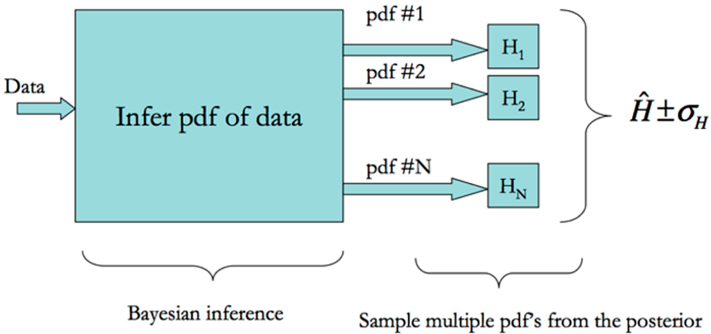
Figure 1.
This schematic illustrates the procedure for estimating entropy as well as the uncertainty from data. First the number of bins is selected using the mode of the logarithm of the Dirichlet posterior in Equation (15). The Dirichlet posterior is then sampled resulting in multiple estimates of the pdf. The entropy of each pdf is estimated and the mean and standard deviation computed and reported.
As previously described, this method is known to produce biases, especially as higher dimensions are considered. There are a couple of reasons for this. As the pdf is modeled by a uniform distribution within a single bin, this corresponds to the maximum entropy for that bin. Additionally, Equation (18) tells us that, even if there is no data sample in a specific bin, an artificial amount β is added to the average bin probability. On the other hand, this addition mitigates the entropy underestimation encountered in the case of many empty bins, which is prevalent in higher dimensions. Moreover, the TE is estimated by the addition and subtraction of the marginal and joint Shannon entropies, as shown in Equation (16). Prichard and Theiler describe the artifacts originating from this summation procedure and advise using KDE methods instead [25]. However, before considering the KDE method, we discuss an alternative histogram method that has been proposed to overcome some of the drawbacks of the fixed-bin-width histogram approaches. In addition to the conjugate pairs of multinomial likelihood and Dirichlet prior model, the research topic of exploring other models has always been interesting. In addition to this conjugate pair, optimal binning in the case of other models, such as that of [24] including a mixture of Dirichlets provides a challenging research for optimal binning of data with the goal of efficient pdf estimation from the data.
2.2. Adaptive Bin-Width Histogram Approaches
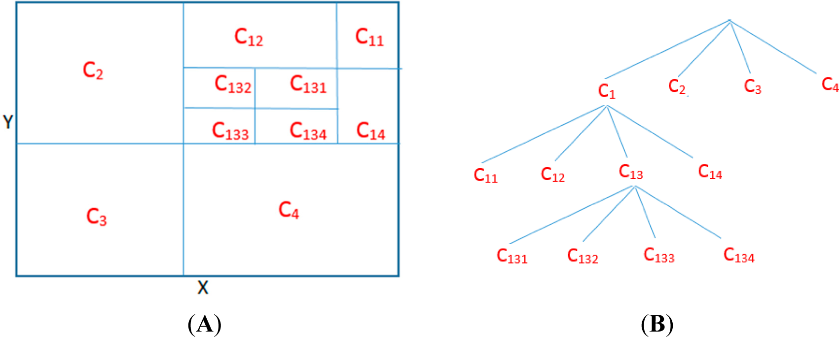
The fixed bin-width histogram approaches are not very effective for estimating information-theoretic quantities from data due to the inaccurate filling of the bins with zero sampling frequency. Instead of generating a model based on bins with equal width, one can design a model consisting of bins with varying widths, determined according to a statistical criterion. Fraser and Swinney [34] and Darbellay and Vajda [35] proposed the adaptive partitioning of the observation space into cells using the latter approach and estimated the mutual information (MI) directly. Here, we will focus on the method proposed by Darbellay and Vajda. This approach relies on iteratively partitioning the cells on the observation space, based on a chi-square statistical test to ensure conditional independence of the proposed partitioned cells from the rest of the cells. We explain the details of this method schematically on Figure 2. Here, observation space of (X, Y) is shown by the largest rectangle. The partitioning of the observation space is done as follows:
- Initially, we start with the largest rectangle containing all data samples.
- Any cell containing less than two observations (data pairs) is not partitioned. The cell, which is partitioned into smaller blocks, is known as the parent cell; whereas each smaller block after partitioning is named as a child cell.
- Every cell containing at least two observations is partitioned by dividing each one of its edges into two halves. It means four new cells are generated (according to the independence test, which will be described below).
- In order to test whether we need to partition the upper cell (parent cell) into more cells (child cells), we rely on the Chi-Square test of independence, where the null hypothesis is phrased as follows:
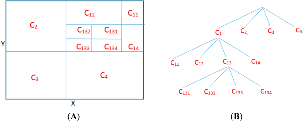
Figure 2.
Illustration of the Adaptive Partitioning algorithm of Darbellay and Vajda (A) The observation space of two-dimensional data (X,Y) and its illustrative partitioning according to the independence test; (B) The corresponding tree showing the partitioning of each cell.
H0: Sample numbers N1, N2, N3, N4 in four child cells are similar (in other words, the sample distribution in the parent cell was uniform)
The Chi-Square (χ2) test statistic for a 5% significance level with 3 degrees of freedom is given as follows:
If we happen to find that T > 7.81, we decide that the numbers of samples in each child cell are not similar and therefore we continue partitioning. Otherwise, we conclude that the numbers are similar and partitioning is stopped at this level. The data samples in this cell are used in the MI estimation.
In this method, the level of statistical significance can be chosen according to the design, thus raising as a parameter to be tuned according to the application. After the partitioning is completed, the MI is estimated as shown below:
where N denotes the total number of data samples with Ni showing the subset of these samples that fall into the ith cell, Ci, after the partitioning process is completed. Above, Nx,i and Ny,i represent the numbers of observations having the same x and y coordinates as observations in the cell Ci, respectively. The partitioning process is illustrated below using a similar discussion to that in [35]. The observation space is first divided into four child cells, namely C1, C2, C3, C4, to maintain equiprobable distributions in each cell. This forms the first set of branches shown in Figure 2b. Then, according to the independence test, C1 is divided into four cells whereas C2, C3, C4 are retained to be included in the MI estimation and they are not divided into more child cells, forming the second layer of the partitioning tree shown in Figure 2b. Finally, the third child cell of partition C3 is divided into four child cells, namely C131, C132, C133 and C134. In the last step, each cell is utilized in the MI estimation formula given by Equation (20). It should be noted that the partitioning is performed symbolically here for the sake of a better explanation without showing the actual data samples on the observation space, as done in [35].
As a result, finer resolution is used to describe larger MI regions and lower resolution is used for smaller MI regions [35]. Having estimated the MI from the data efficiently, the TE can be calculated using the expressions from [19] by:
where
denotes the MI between Xi+1 and the joint process denoted by
[19].
Because the MI is estimated more efficiently by this method, the overall TE estimation becomes less biased compared to the previous methods. However, the subtraction operation involved in Equation (21) can still produce a significant bias in the TE calculations. To overcome problems related to the addition and subtraction of information-theoretic quantities, KDE estimation methods have been utilized in the literature to estimate MI and redundancies [25], and TE in [49].
2.3. Kernel Density Estimation Methods
Kernel Density Estimation (KDE) is utilized to produce a smoothed pdf estimation using the data samples, which stands in contrast to the histogram model which has sharp edges resulting from a uniform distribution within each bin. In this method, a preselected distribution of values around each data sample is summed to obtain an overall, smoother pdf in the data range. This preselected distribution of values within a certain range is known as a “kernel”. Some of the most commonly used kernels are “Epanechnikov”, “Rectangular” and “Gaussian” [28]. Each kernel can be thought of as a window with a bandwidth or radius. Prichard and Theiler [25] showed that KDE can also be utilized to estimate entropy by the computation of the generalized correlation integral [7], which is approximated by the correlation sum. Even if a rectangular kernel is used, the resulting entropy estimation is more accurate compared to the histogram approach as discussed in [25]. In this method, entropies are estimated by first calculating the correlation sums through the Grassberger-Procaccia (GP) algorithm or some other effective procedure. Interested readers are referred to [31–33] for a detailed description of the algorithm. Here, the joint probabilities in the TE expression (6) can be estimated from data by the following equation, which is known as the generalized correlation sum [7]:
where Θ(x > 0)=1; Θ(x < 0)=0 is the Heaviside function and ε is the radius around each data sample. In Equation (22), we count the number of neighboring data samples which are within ε distance. As a distance measure, the maximum norm, denoted║·║, has been selected here, but the Euclidean norm could also be utilized. On the right-hand side of Equation (22),
gives the mean probability that the states at two different indices (i and m) are within ε distance of each other. Using Equation (22), the TE can be expressed as [49,50]:
where ⟨.⟩ denotes the expectation [50].
The problem is that this method also has a free parameter, the radius value, ε, which must be selected to estimate the neighborhoods. Choosing this radius is similar to choosing the fixed bin width in a histogram. We utilize the Grassberger-Procaccia algorithm to plot log ε versus. The linear section along the resulting curve is used to select the radius ε. However, picking a radius value from any part of the linear section of the log ε versus curve appears to make the results sensitive over the broad range of possible values. This is explored in the following section and the benefit of exploring an appropriate radius range with the help of the embedding dimension selection is pointed out.
2.3.1. Selection of the Radius with the Embedding Dimensions in Kernel Density Estimation (KDE) Method
Here we explain a method to select the radius based on the above discussion in concert with the choice of the embedding dimensions k and l, based on the discussions in [14]. We demonstrate this procedure on a system consisting of a pair of linearly-coupled, autoregressive signals [51]:
where
denotes the normal distribution with mean μ and standard deviation σ and the constant c denotes the coupling coefficient. First, we generate the log ε versus
curve. The log ε versus
curve is displayed in Figure 3 for different k values and c = 1.
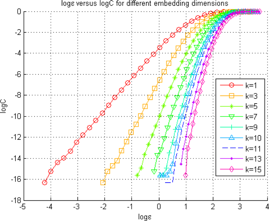
Figure 3.
Exploration of the optimal radius for the KDE of a pdf using the Grassberger-Procaccia method. The figure illustrates the Correlation Sum, defined in Equation (22), estimated at different radius values represented by ε for the coupled AR model.
Here, l = 1 is selected [14]. It is known that the optimal radius lies in the linear region of these curves, where its logarithm is a point on the horizontal axis [14]. Above, we notice that the range of the radius values corresponding to the linear section of each curve varies significantly. As the k value increases, the linear region for each curve moves right, toward higher ε values [33]. With the increasing embedding dimensions, the embedding vectors include data, which are sampled with a lower frequency, i.e., undersampling, leading to an increase in ε to achieve the same correlation sum obtained with a smaller radius. For example, a set of radius values within the range of −3≤ log ε ≤ 0 provides the linear section of the log C curve for k = 1, whereas these values are not within the range of radius values used in forming the log C -log ε curve for an embedding dimension of k = 10. Thus, selection of an embedding dimension k first and then a radius value from the corresponding linear region on the curve can help us search for the radius in a more constrained and efficient way.
As seen in Figure 3, we end up with different radius ranges to select, based on the determination of the embedding dimension, k. Sabesan et al. [14] provide an approach to select the radius (ε) and k together.
According to [14,52], the embedding dimension, k, can be selected by considering the first local minimum of the Time-Lagged MI (TLMI) of the destination signal, followed by the determination of a radius value. The radius is selected such that it falls into the linear region of the curve for the corresponding k value, given in Figure 3. The k value, corresponding to the first local minima of MI(k), provides us with the time-lag k, where the statistical dependency between the current sample xi and its k past value xi-k is small. TLMI is defined by the following equation for the AR signal given in Equation (24):
Below, we provide an estimate of the MI(k) of the AR signal, xi, for different time lags k ∈ [1,…,50]. The adaptive partitioning algorithm of Darbellay and Vajda [35] was utilized to estimate the MI. As the MI is not bounded from above, we normalize its values between 0 and 1 as recommended in the literature, using the following formula [53]:
In Figure 4, we show the normalized MI for different lags after taking an ensemble of 10 members of the AR process x and utilizing an averaging to estimate MI.
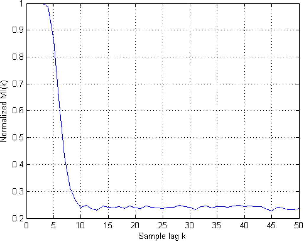
Figure 4.
Ensemble averaged and normalized Time-lagged MI(k). As described in the text, the first local minima of the MI leads to the condition k = 10.
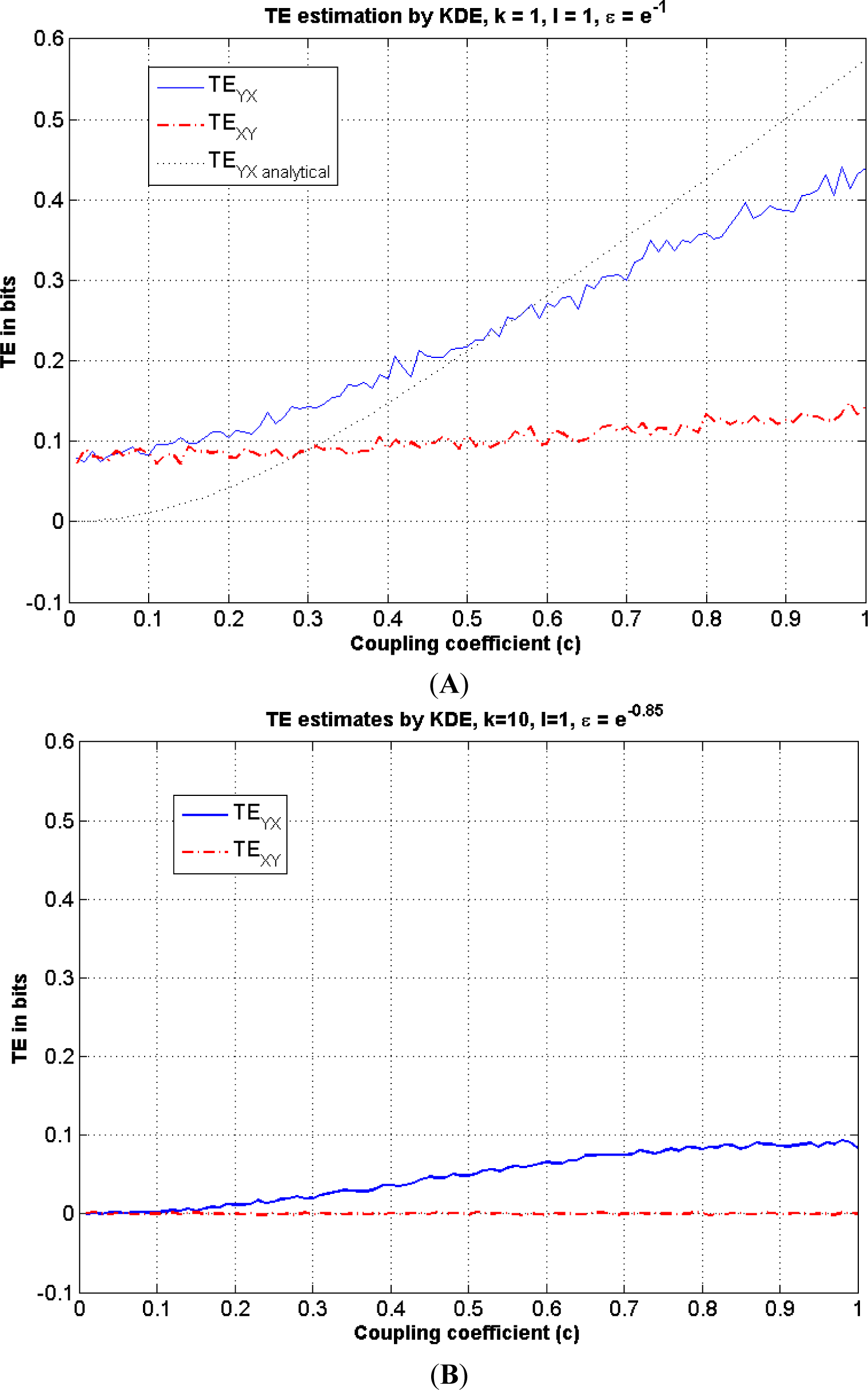
Above, the first local minimum value of MI(k) is obtained at k = 10. Thus, we turn to Figure 3 to select a radius value on the linear region of the curve with the embedding dimension k = 10. This region can be described by the following values: 0.8 ≤ log å ≤ 1.4. Thus, we can choose k = 10 and log ε =0.85 along with l = 1. If k = l = 1 is selected, the corresponding linear region on Figure 3 changes and a selection of log ε=−1 can be chosen, instead. Once the radius and the embedding dimensions are determined, TE is estimated by Equation (23) using the correlation sums. These estimates are illustrated in Figure 5A,B for k = l = 1 and k = l0, l = 1; respectively.
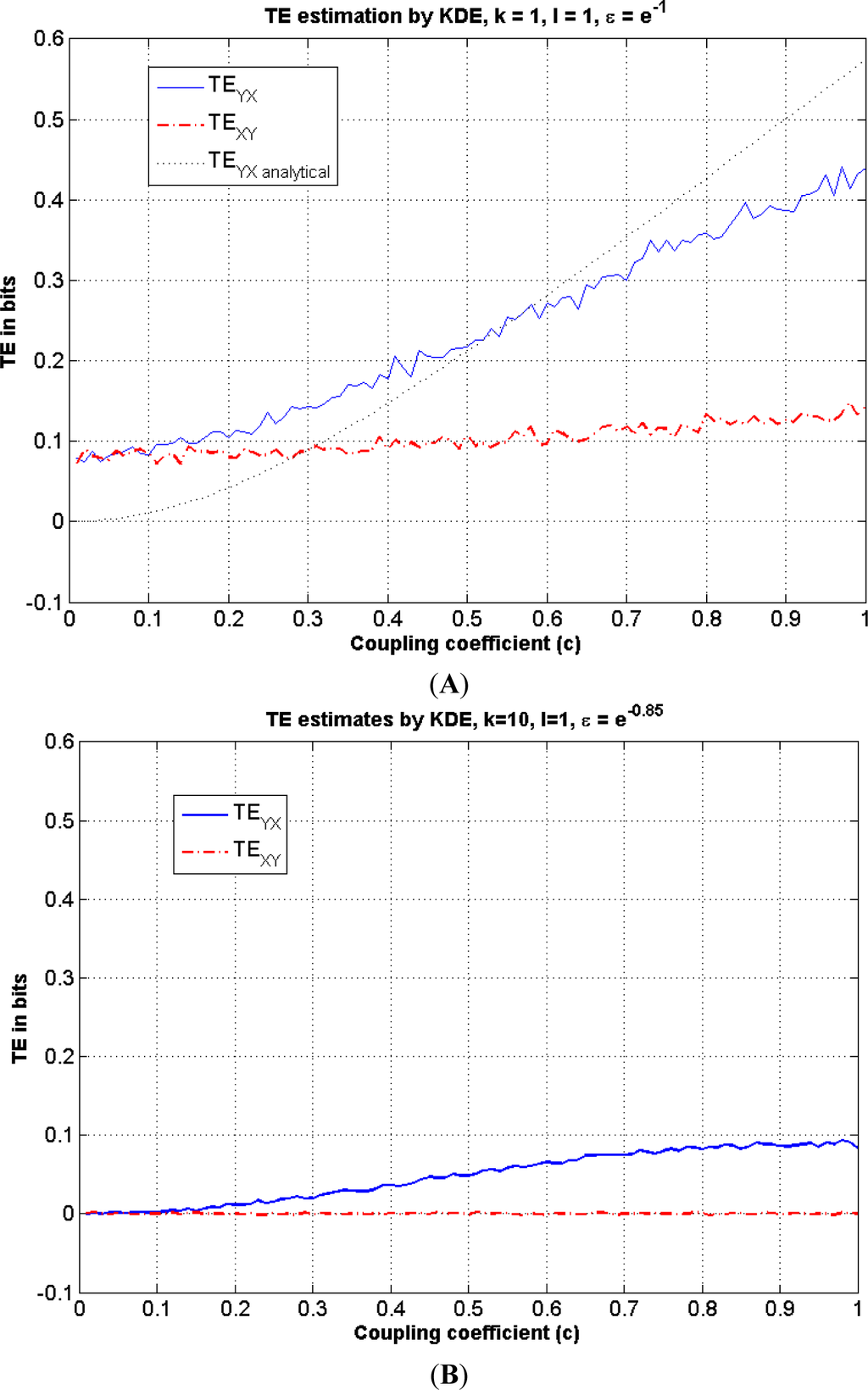
Figure 5.
This figure illustrates TE estimation versus the coupling coefficient c in Equation (24) using the KDE method. (A) Both TEYX (blue-solid) and TEXY (red-dash dot) are estimated using the KDE method and illustrated along with the analytical solution (black-dotted) for k = l = 1. As there is no coupling from X to Y, analytically TEXY =0; (B) TEYX (blue-solid) and TEXY (red-dash dot) are estimated using the KDE method for k = 10, l = 1.
In the next section, we will elaborate on the performance of the three methods used in TE estimation and emphasize the goal of our approach, which is to use all three methods together to fine tune their specific parameters.
3. Experiments
In the preceding section, we described three different methods for estimating the TE from data, namely: the Generalized Knuth method, the adaptive bin-width histogram and the KDE method. We emphasized that we can compute different TE values by these three different methods, as the TE estimations depend on various factors, such as the value of the selected fixed bin-width, the bias resulting due to the subtraction and addition of various Shannon entropies, embedding dimensions and the value of the chosen KDE radius value. Due to this uncertainty in the TE estimations, we propose to use these three main techniques together to compute the TE values and to consistently identify the direction of relative information flows between two variables. With this approach, if one of the techniques does not agree with the others in terms of the direction of information flows between the variables, we determine that we need to fine tune the relevant parameters until all three methods agree with each other in the estimation of the NetTE direction between each pair of variables. The NetTE between two variables X and Y is defined to be the difference between TEXY and TEYX, which is defined as the difference of the TE magnitudes with opposite directions between X and Y:
The NetTE allows us to compare the relative values of information flow in both directions and conclude which flow is larger than the other, giving a sense of main interaction direction between the two variables X and Y.
In order to use three methods together, we demonstrate our procedure on a synthetic dataset generated by a bivariate autoregressive model given by Equation (24). In Section 2.3.1, we have already described the KDE method using this autoregressive model example and we have explored different radius values in the KDE method by utilizing the Grassberger-Procaccia approach in conjunction with different selections of k values. In Section 3.1, we continue demonstrating the results using the same bivariate autoregressive model. We focus on the analysis of the adaptive partitioning and the Generalized Knuth methods. First, we analyze the performance of the adaptive partitioning method at a preferred statistical significance level. Then, we propose to investigate different β values to estimate the optimal fixed bin-width using Equation (15) in the Generalized Knuth method.
If an information flow direction consensus is not reached among the three methods, we try different values for the fine-tuning parameters until we get a consensus in the NetTE directions.
When each method has been fine-tuned to produce the same NetTE estimate, we conclude that the information flow direction has been correctly identified.
In Section 3.2, we apply our procedure to explore the information flow among the variables of the nonlinear dynamical system used by Lorenz to model an atmospheric convection cell.
3.1. Linearly-Coupled Bivariate Autoregressive Model
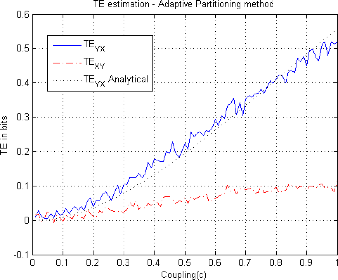
In this section, we apply the adaptive partitioning and the Generalized Knuth methods to estimate the TE among the processes defined by the same bivariate linearly-coupled autoregressive model (with variable coupling values) given by the equations in Equation (24). We demonstrate the performance of each TE estimation method using an ensemble of 10 members to average. The length of the synthetically generated processes is taken to be 1000 samples after eliminating the first 10,000 samples as the transient. For each method, TE estimations versus the value of coupling coefficients are shown in Figures 5–7 for both directions between processes X and Y. It should be noted that the process X is coupled to Y through coefficient c. Thus, there is no information flow from X to Y for this example, i.e., TEXY = 0 analytically. The analytical values of TEYX have been obtained using the equations in [19] for k = 1 and l = 1. The performance of the three methods have been compared for the case of k = 1 and l = 1.
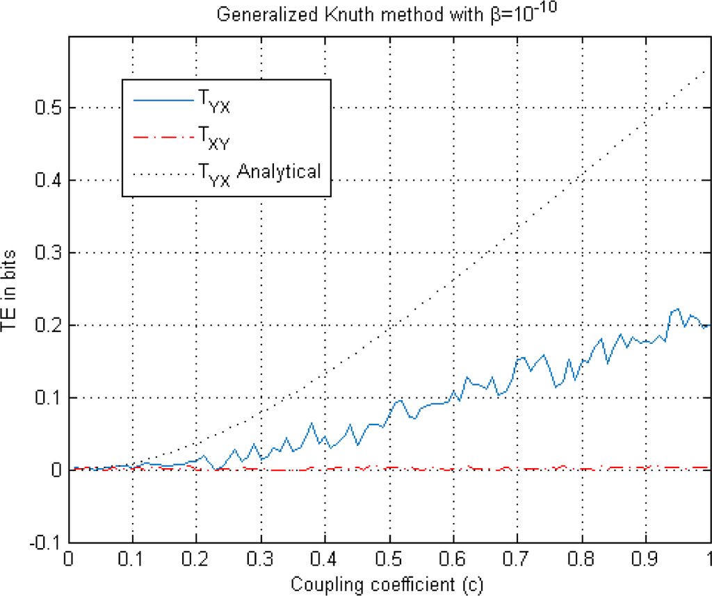
Figure 7.
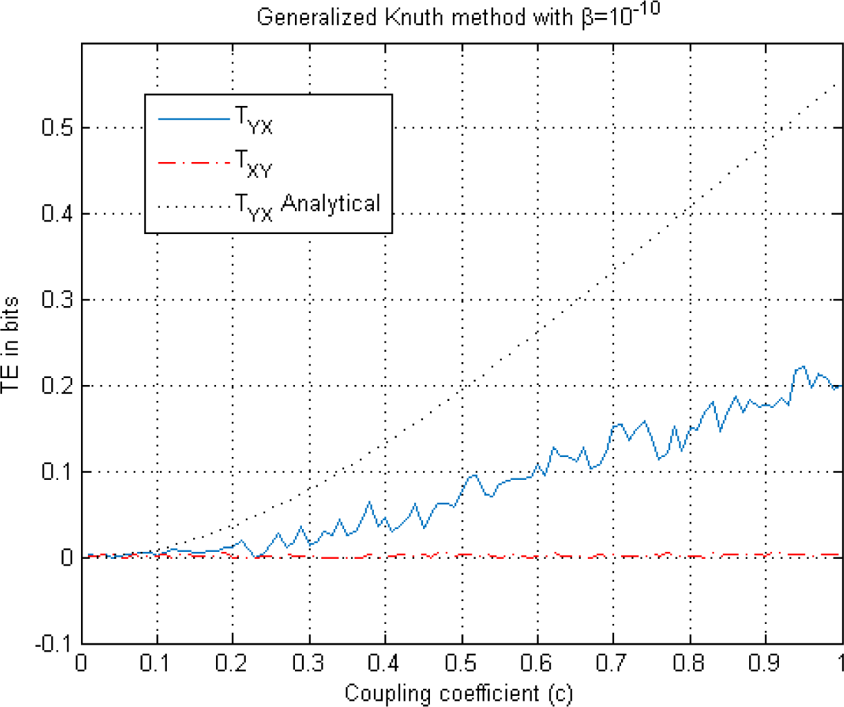
This figure illustrates TE estimation versus the coupling coefficient c in Equation (24) using the Generalized Knuth method. Both TEYX (blue solid) and TEXY (red-dash dot) are estimated for β = 10−10 and illustrated along with the analytical solution (black dotted) where k = l = 1 is chosen.
Below, TE is estimated for both directions using coupling values ranging from c=0.01 to c=1 in Equation (24). The information flows are consistently estimated to be in the same direction for all three methods, i.e., TEYX≥TEXY. If we compare the magnitudes of these TE estimates, we observe that the biases between the analytic solution and the TEYX of the adaptive partitioning method, KDE and the Generalized Knuth method increase as the coefficient of the coupling in the autoregressive model increases to c = 1.
Above, we demonstrate the TE estimations using the KDE method with different embedding dimensions and different radius values. In Figure 5A, B, we observe that the directions of each TE can be estimated correctly, i.e., TEYX≥TEXY. for the model given in Equation (24), demonstrating that we can obtain the same information flow directions, but with different bias values.
When the magnitudes of the TEYX estimates are compared in Figures 5A and 6, we observe bias both in TEYX and TEXY, whereas there is no bias in the TEXY estimate in the Generalized Knuth method using β =10−10. On the other hand, the adaptive partitioning method provides the least bias for TEYX whereas KDE seems to produce larger bias for low coupling values and lower bias for high coupling values in Figure 5A, compared to the Generalized Knuth method with β =10−10 in Figure 7.
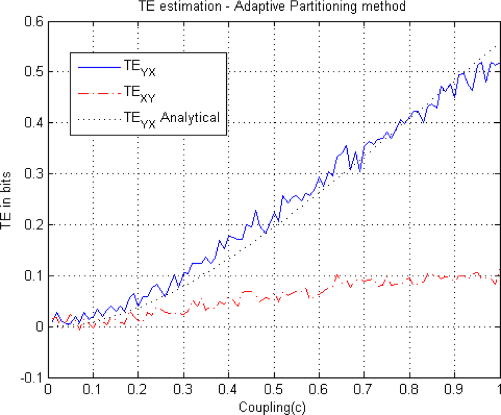
Figure 6.
This figure illustrates TE estimation versus the coupling coefficient c in Equation (24) using the adaptive partitioning method. Both TEYX (blue-solid) and TEXY (red-dash dot) are estimated using the adaptive partitioning method and illustrated along with the analytical solution (black-dotted). As there is no coupling from X to Y, analytically TEXY =0. A statistical significance level of 5% has been utilized in the χ2 test Equation (19) for a decision of partitioning with k = l = 1.
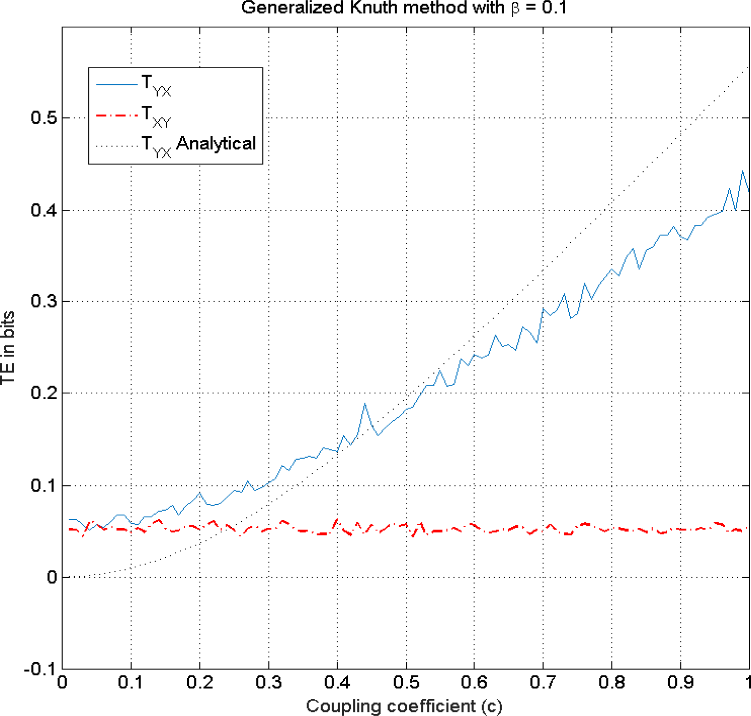
For example, for c = 1, we note from the three graphs that the estimated transfer entropies are TEYX ≅ 0.52, TEYX ≅ 0.43, TEYX ≅ 0.2, for the adaptive partitioning, the KDE with k = l = 1 and the Generalized Knuth method with β = 10−10, respectively. As the bias is the difference between the analytical value (TEYX = 0.55 for k = 1 = 1) and the estimates, it obtains its largest value in the case of the Generalized Knuth method with β = 10−10. On the other hand, we know that there is no information flow from the variable X to variable Y, i.e., TEXY = 0. This fact is reflected in Figure 7, but not in Figures 5A and 6 where TExy is estimated to be non-zero, implying bias. As the same computation is also utilized to estimate TEYX (in the other direction), we choose to analyze the NetTE, which equals the difference between TEYX and TEXY, which is defined in Equation (27). Before comparing the NetTE obtained by each method, we present the performance of the proposed Generalized Knuth method for different β values.
3.1.1. Fine-Tuning the Generalized Knuth Method
In this sub-section, we investigate the effect of β on the TE estimation bias in the case of the Generalized Knuth method. The piecewise-constant model of the Generalized Knuth method approaches a pure likelihood-dependent model, which has almost a constant value as β goes to zero in Equation (18). In this case, the mean posterior bin heights approach their frequencies in a bin, i.e.,
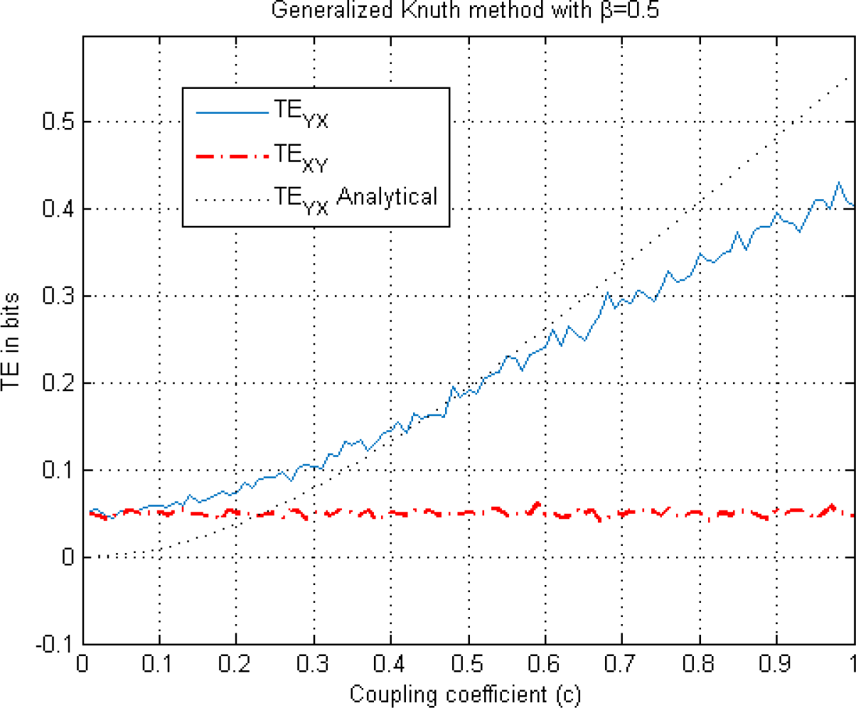
. In this particular case, empty bins of the histogram cause large biases in entropy estimation, especially in higher dimensions as the data becomes sparser. This approach can only become unbiased asymptotically [54]. However, as shown in Equation (18), the Dirichlet prior with exponent β artificially fills each bin by an amount, β, reducing the bias problem. In Appendix III, Figure A3 illustrates the effect of the free parameter β on the performance of the marginal and joint entropy estimates. We find that the entropy estimates fall within one to two standard deviations for β ≅ 0.1. The performance degrades for much smaller and much larger β values. Figures 8 and 9 illustrate less bias in TEYX estimates for β =0.1 and β =0.5 unlike the case in shown in Figure 7 where we use β=10−10. However, the bias increases for low coupling values in these two cases. To illustrate the net effect of the bias, we explore NetTE estimates of Equation (27) for these cases in Section 3.1.2.
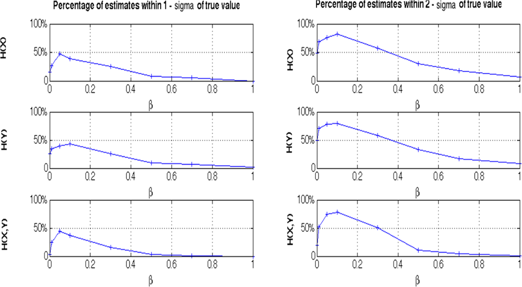
Figure A.3.
Percentage performance (one- and two-standard deviation confidence intervals) of marginal and joint entropy estimates as a function of β.
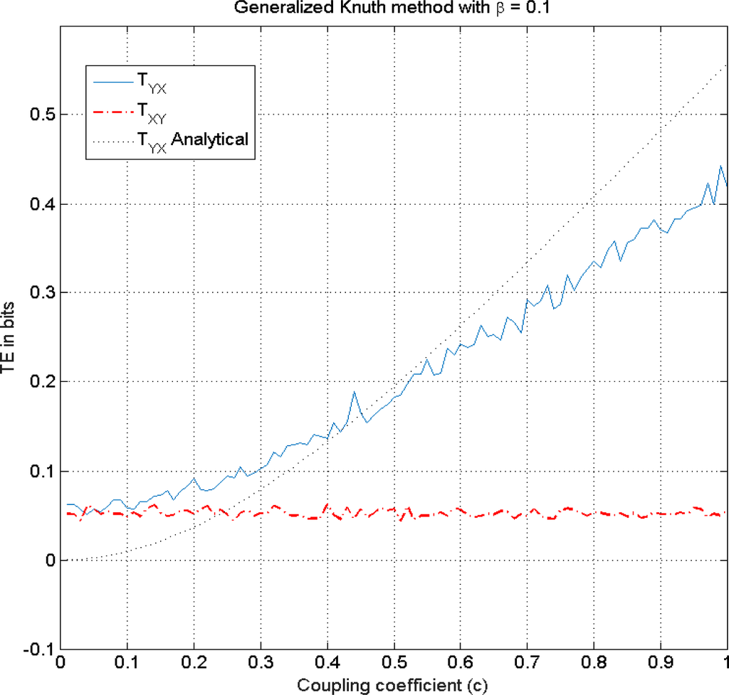
Figure 8.
This figure illustrates TE estimation versus the coupling coefficient c in Equation (24) using the Generalized Knuth method method for β = 0.1, k =l=1. These are illustrated along with the analytical solution.
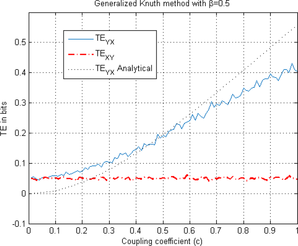
Figure 9.
This figure illustrates TE estimation versus the coupling coefficient c in Equation (24) using the generalized piecewise-constant method (Knuth method) for β =0.5, k =l =1. These are illustrated along with the analytical solution.
3.1.2. Analysis of NetTE for the Bivariate AR Model
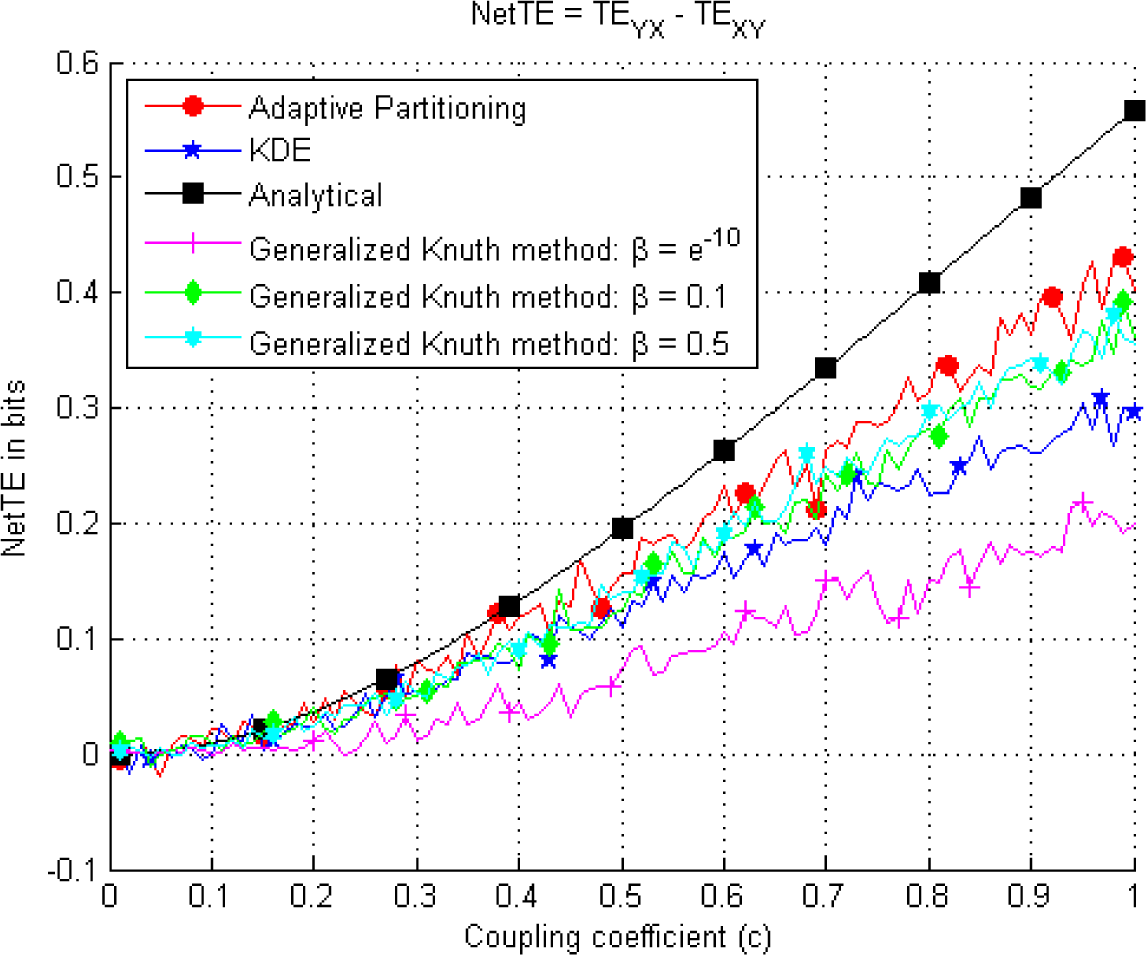
Since we are mainly interested in the direction of the information flow, we show that the estimation of the NetTE values exhibit more quantitative similarity among the methods for the case where k = l = 1 (Figure 10).

Figure 10.
This figure illustrates the NetTE difference, given by Equation (27) between each pair of variables in Equation (24). Estimations are performed using all three methods and considering different β values in the case of the Generalized Knuth method.
In the KDE (Figure 5A), Adaptive partitioning (Figure 6) and the Generalized Knuth method with β =0.1 and β =0.5, (Figures 8 and 9) a non-zero TEXY is observed. The NetTE between the variables X and Y of the bivariate auroregressive model in Equation (24) still behaves similarly giving a net information flow in the direction of the coupling from Y to X as expected. Thus, in this case we find that the NetTE behaves in the same way, even though the individual TE estimates of each method have different biases. Above, we observe that the NetTE estimate of the adaptive partitioning outperforms the Generalized Knuth method with β =0.1 and β =0.5 and KDE. The largest bias in NetTE is achieved by the Generalized Knuth method with β =10−10. However, all methods agree that the information flow from Y to X is greater than that of X to Y, which is in agreement with the theoretical result obtained from Equation (24) using the equations in [19]. In the literature, the bias in the estimation has been obtained using surrogates of TE’s estimated by shuffling the data samples [38]. These approaches will be explored in future work.
3.2. Lorenz System
In this section, the three methods of Section 2 are applied to a more challenging problem involving the detection of the direction of information flow among the three components of the Lorenz system, which is a simplified atmospheric circulation model that exhibits significant non-linear behavior. The Lorenz system is defined by a set of three coupled first-order differential equations [41]:
where σ = 10,b = 8⁄3, R = 24 (sub − chaotic) or R = 28 (chaotic). These equations derive from a simple model of an atmospheric convection cell, where the variables x, y, and z denote the convective velocity, vertical temperature difference and the mean convective heat flow, respectively. These equations are used to generate a synthetic time series, which is then used to test our TE estimation procedure. In the literature, the estimation of the TE of two Lorenz systems with nonlinear couplings have found applications in neuroscience [14,39,55]. Here, we explore the performance of our approach on a single Lorenz system which is not coupled to another one. Our goal is to estimate the interactions among the three variables of a single Lorenz system–not coupling from one system to another.
In our experiments, we tested the adaptive partitioning, KDE and Generalized Knuth methods in the case where the Rayleigh number, R = 28, which is well-known to result in chaotic dynamics and also for the sub-chaotic case where R = 24. For each variable, we generated 15,000 samples and used the last 5000 samples after the transient using a Runge-Kutta-based differential equation solver in MATLAB (ode45). Both in the chaotic and sub-chaotic cases, β = 0.1 was used at the Generalized Knuth method and a 5% significance level was selected in the adaptive partitioning method. Embedding dimensions of k = l = 1 have been selected in these two methods.
The embedding dimension values were implemented according to Section 2.3.2 at the KDE method: The log ε versus curves have been estimated for the chaotic and sub-chaotic cases.
In the chaotic case, the first minimum of TLMI was found to be at k = 17 and ε =e−1 occured in the middle of the radii range of the linear part of the curve. The value of l = 1 was selected for both the chaotic and sub-chaotic cases. The curves for different k values have been illustrated in Figure 11 for the analysis of the interaction between X and Y. Similar curves have been observed for the analysis of the interactions between the other pairs in the model.
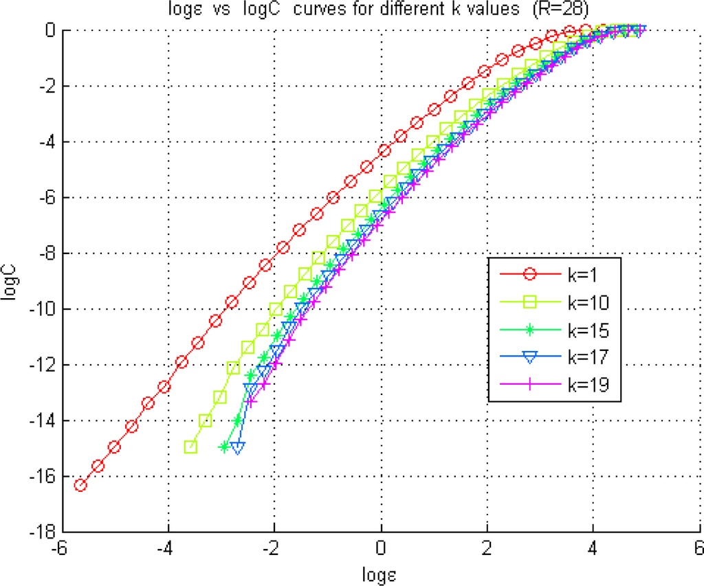
Figure 11.
Exploration of the optimal radius for the KDE of a pdf using the Grassberger-Procaccia method. The figure illustrates the Correlation Sum (22) estimated at different radius values represented by ε for the Lorenz model in the chaotic regime (R = 28).
In the sub-chaotic case, values around k = 15 have been observed to provide the first local minimum of TLMI(k). However, the NetTE direction consistency cannot be obtained with the other two techniques, namely, the adaptive partitioning and the Generalized Knuth method. Therefore, as we propose in our method, k value has been fine-tuned along with the radius until we obtain consistency of NetTE directions among the three methods. Selection of k = 3, l=1, ε = e−2 has provided this consistency, where the NetTE directions are illustrated in Figure 15. Figure 12 illustrates log ε versus curves used in the selection of the appropriate region for ε, in the sub-chaotic case.

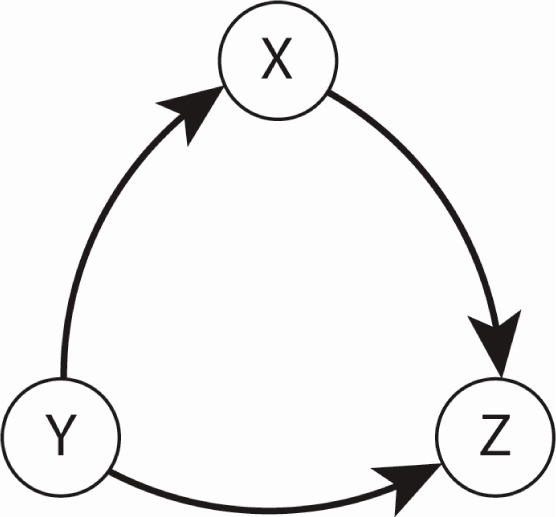
Figure 15.
Information flow directions among the variables of the Lorenz equations, where X, Y, Z denote the velocity, temperature difference and the heat flow, respectively, in the case of the atmospheric convection roll model. These are also the NetTE directions, showing the larger influence among the bi-directional flows.
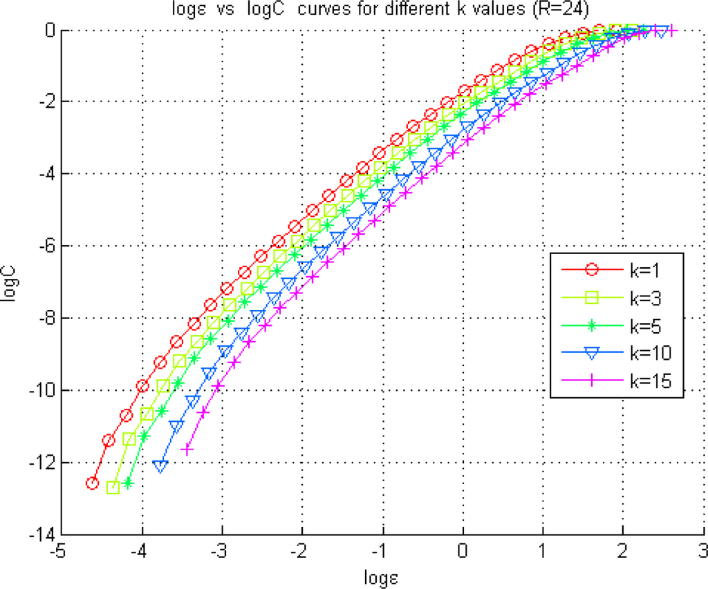
Figure 12.
Exploration of the optimal radius for the KDE of a pdf using the Grassberger-Procaccia method. The figure illustrates the Correlation Sum (22) estimated at different radius values represented by ε for the Lorenz model in the sub-chaotic regime (R = 24).
We estimated TE for both directions for each pair of variables (x,y), (x,z), and (y, z) using each of the three methods described in Section 2. Similar to the MI normalization of Equation (26) recommended in [53], we adapt the normalization for the NetTE as follows:
where δXY denotes the normalized NetTE between variables X and Y, having values in the range of [0,1]. In Figures 13 and 14, we illustrate the information flow between each pair of the Lorenz equation variables using both the un-normalized TE values obtained by the each of the three methods and the normalized NetTE estimates showing the net information flow between any pair of variables.
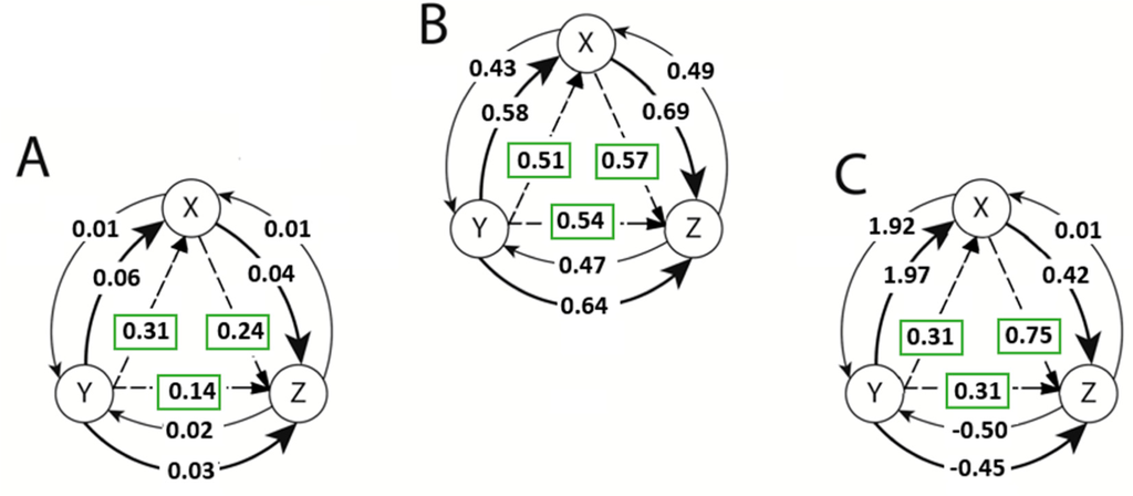
Figure 13.
The un-normalized TE estimates between the variables of the Lorenz equations defined in Equation (28) for the chaotic case (R = 28) along with the normalized NetTE direction and magnitudes. Estimations were obtained using (A) Kernel Density Estimate method with k = 17, l = 1, ε =e−1; (B) Generalized Knuth method method with β=0.1, k=l =1; and (C) Adaptive Partitioning method with 5% significance level and k = l = 1. Solid arrows denote the information flow (or TE) from X to Y or Y to X. Dashed lines show the direction of the normalized NetTE estimates.
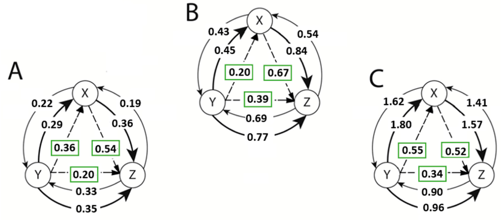
Figure 14.
The un-normalized TE estimates between the variables of the Lorenz equations defined in Equation (28) for the sub-chaotic case (R = 24) along with the normalized NetTE direction and magnitudes. Estimations were obtained using: (A) Kernel Density Estimate method with k =3, l=1, ε = e−2; (B) Generalized Knuth method where β =0.1, k = l =1; (C) Adaptive Partitioning method with 5% significance level and k = l =1. Solid arrows denote the information flow (or TE) from X to Y or Y to X. Dashed lines illustrate the direction of the normalized NetTE estimates.
Above, the un-normalized TE values are denoted by solid lines between each pair of variables. Also, the normalized NetTE estimates (29) are illustrated with dashed lines. The direction of the NetTE has the same direction as the maximum of two un-normalized TE estimates between each pair, the magnitudes of which are shown in rectangles. For example, in the case of the adaptive partitioning method, the un-normalized TE values are estimated to be TEYZ =−0.45 and TEZY =−0.50 between variables Y and Z, due to the biases originating from the subtraction used in Equation (21). However, the normalized NetTE is estimated to be
and shows a net information flow from variable Y to Z. Thus, we conclude that variable Y affects variable Z.
In Figure 14, we illustrate the estimates of TE’s between each variable of the Lorenz Equation (28) in sub-chaotic regime with R = 24.
Above, we demonstrated the concept of our method: If the directions of information flows are not consistent with the three methods, then we can explore new parameter values to provide consistency in the directions. Above, for the selected parameters, the Generalized Knuth method and the adaptive partitioning provided consistent NetTE directions between the pairs of variables in the chaotic case. However, in the sub-chaotic case, we needed to explore a new parameter set for the KDE method as the NetTE directions were different than the other two consistent methods.
Based on the fact that the directions of the NetTE estimations obtained using each of the three methods agree, we conclude that information flow direction between the pairs of the Lorenz equation variables are as shown in Figure 15.
Note that these information flow directions are not only not obvious, but also not obviously obtainable, given the Lorenz system equations in Equation (28) despite the fact that these equations comprise a complete description of the system (sensitive dependence on initial conditions not withstanding). However, given the fact that this system of equations is derived from a well-understood physical system, one can evaluate these results based on the corresponding physics. In an atmospheric convection roll, it is known that both the velocity (X) and the heat flow (Z) are driven by the temperature difference (Y), and that it is the velocity (X) that mediates the heat flow (Z) in the system. This demonstrates that complex nonlinear relationships between different subsystems can be revealed by a TE analysis of the time series of the system variables. Furthermore, such an analysis reveals information about the system that is not readily accessible even with an analytic model, such as Equation (28), in hand.
4. Conclusions
Complex systems, such as the Earth’s climate, the human brain, and a nation’s economy, possess numerous subsystems, which not only interact in a highly nonlinear fashion, but also interact differently at different scales due to multiple feedback mechanisms. Analyzing these complex relationships in an attempt to better understand the physics underlying the observed behavior poses a serious challenge. Traditional methods, such as correlation analysis or PCA are inadequate due to the fact that they are designed for linear systems. TE has been demonstrated to be a potentially effective tool for complex systems consisting of nonlinearly-interacting subsystems due to its ability to estimate asymmetric information flow at different scales, which is indicative of cause and effect relationships. However, there are serious numerical challenges that need to be overcome before TE can be considered to be a dependable tool for identifying potential causal interactions. In response to this, we have developed a practical approach that involves utilizing three reasonably reliable estimation methods together. Instead of fine tuning the specific parameters of each method blindly, we find a working region where all three methods give the same direction of the information flow. In the case of collective agreement, we conclude that the individual tuning parameters for each method are near their optimal values. This was demonstrated on a bivariate linearly-coupled AR process as well as on the Lorenz system in both the chaotic and sub-chaotic regimes. Our success in deciphering the direction of information flow in the Lorenz system verified—not by the Lorenz system of differential equations—but rather by considering the known underlying physics suggests that this approach has significant promise in investigating and understanding the relationships among different variables in complex systems, such as the Earth’s climate.
Acknowledgments
The first author would like to thank Joseph Lizier for various discussions on TE during the beginning of this research. We also would like to thank three anonymous reviewers for their invaluable comments and suggestions. The first author would like to thank Petr Tichavsky for his code for the estimation of MI given at his web page. Also, we would like to thank NASA Cloud Modeling Analysis Initiative NASA GRANT NNX07AN04G for the support of this research.
Appendix 1
In this Appendix we illustrate, via numerical simulation, the sensitivity of TE estimates on the number of bins used in a histogram model of a pdf. Consider the coupled autoregressive process:
where n1 and n2 are samples of zero mean and unit variance in Gaussian distributions, and c represents the coupling coefficient that couples the two time series equations for x and y. Here, TEXY = 0, as the coupling direction is from Y to X (due to the coupling coefficient c). It was demonstrated by Kaiser and Schreiber ([19]) that the TE can be analytically solved for this system. By choosing the coupling coefficient to be c = 0.5, one finds TEYX = 0.2. Numerical estimates of TE were performed by considering 11 datasets with the number of data points ranging from 10 to 1000. Eleven histograms were constructed for each dataset with the number of bins ranging from 2 to 100, and from these histograms the relevant Shannon entropies were computed. Figure A1.1 illustrates the normalized TEYX values, which are computed using the Shannon entropies in (17), for each combination of N data points and M histogram bins considered. First, note that the estimated TE values range from below 0.1 to above 0.5 where the correct TE value is known to be 0.2 demonstrating that the TE estimates are highly dependent on both the number of data points and the number of bins. Second, note that there is no plateau where TE estimates remain approximately constant—not to mention correct—over a range of histogram bin numbers. For this reason, it is critical to select the correct number of bins in the histogram model of the pdf. However, this is made even more difficult since the entropy is a transform of the model of the pdf itself and therefore the number of bins required to produce the optimal model of the pdf will not be the same as the number of bins resulting in the optimal entropy estimate. This is explored in Appendix 2.
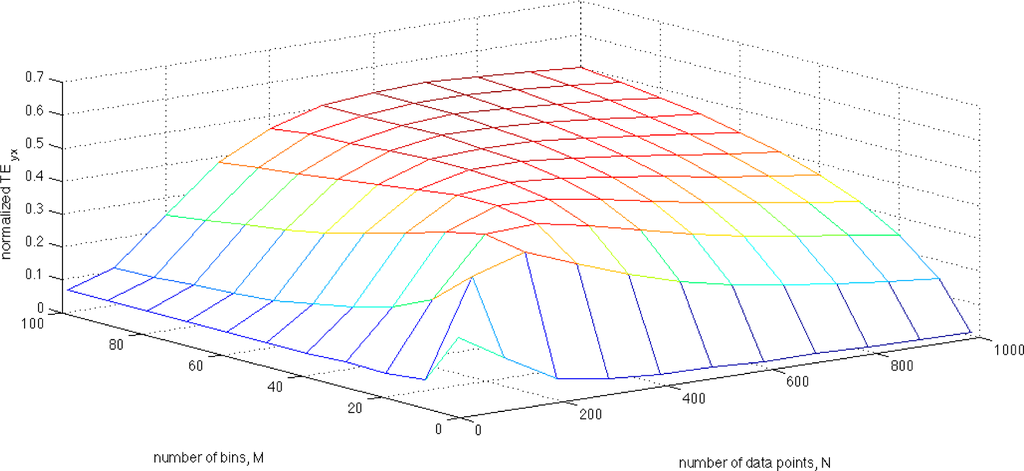
Figure A.1.
This figure illustrates the numerically-estimated normalized transfer entropy, TEYX, of the autoregressive system given in (A.1.1) as a function of varying numbers of data points and histogram bin numbers. To normalize TE, (29) was used as given in the text. Given that the correct value of the transfer entropy is TEYX=0.2, this figure illustrates that the estimation of TE is extremely sensitive to the number of bins chosen for the histogram model of the pdf of the data. (k = l = 1).
Appendix 2
The differential entropy of a variable is estimated by Equation (14). However, due to the finite-precision of numerical calculations in a digital computer, the integral in Equation (14) is approximated by the following discrete summation:
where M denotes the total number of bins used in the histogram and
is the estimate of the continuous pdf of variable X. The Lebesgue measure, m(x), used above is chosen to be the volume V of each bin. Equation (A.2.1) can easily be written for the joint entropies, where
is replaced by its joint pdf counterpart and the volume is estimated for a multi-dimensional bin. In the one-dimensional case, the range of the variable x, is divided into
bins, which is selected to be optimal in Equation (12), and the volume is given by
. We show that the entropy calculation by A.2.1 is biased.
The entropy of the standard Gaussian distribution
with zero mean and unit variance can be analytically computed to be approximately 1.4189. We numerically generated 100 Gaussian-distributed datasets, each with 1000 data points, by sampling from
. Given these 100 datasets, we estimated the 100 corresponding entropy values using the Generalized Knuth method with β = 0.5. We found that 76% and 91% of the entropy estimates were within 1 or 2 standard deviations, respectively, of the true entropy value of 1.4189. However, this means that not every attempt at entropy estimation in this ensemble was successful.
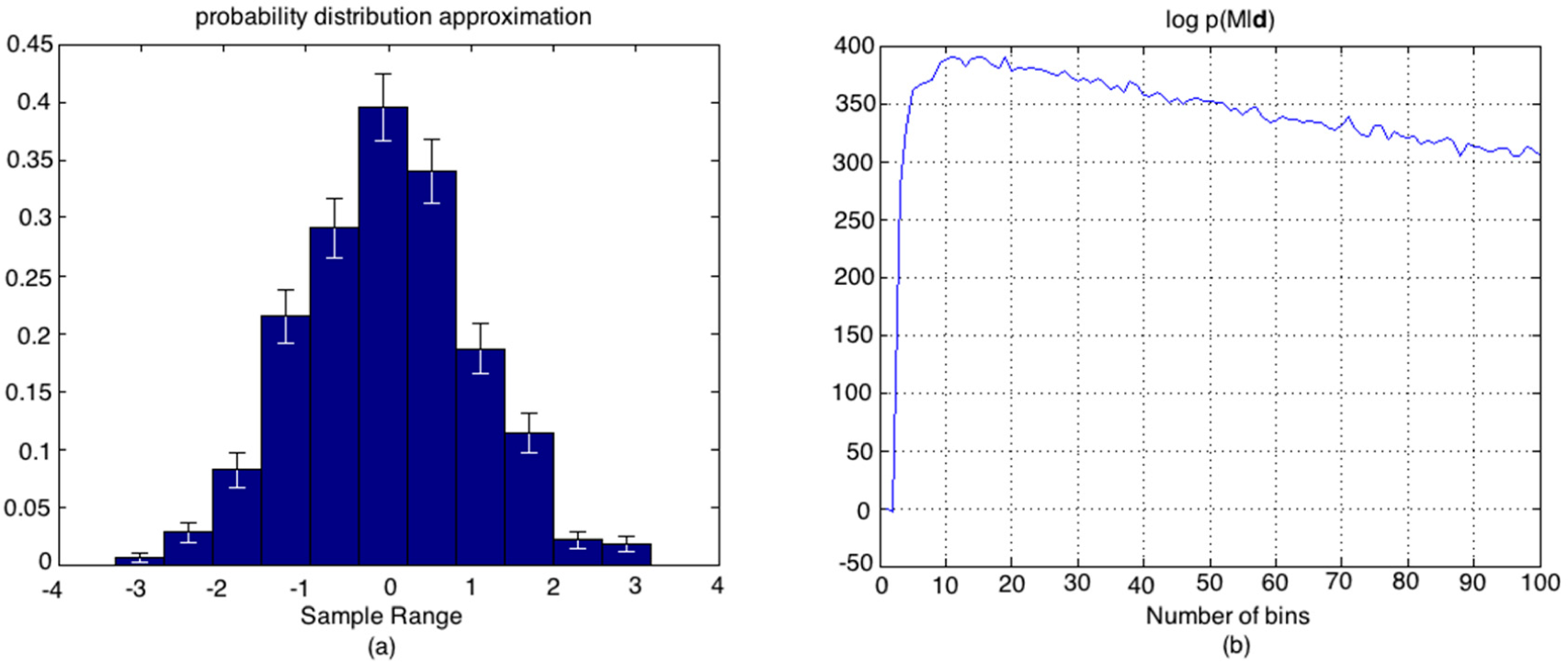
We illustrate this with a specific data set that was found to lie outside of 76% percentile success rate. In this case, the optimal number of bins was estimated to be Mopt =11 using Equation (12). In Figure A.2.1a,b, we illustrate the resulting histogram model of the pdf and the non-normalized log posterior probability of the number of bins in the model given the data.

Figure A.2.1.
(a) Histogram model of the pdf of the data set with error-bars on the bin heights; (b) The non-normalized log posterior probability of the number of bins in the model given the data.
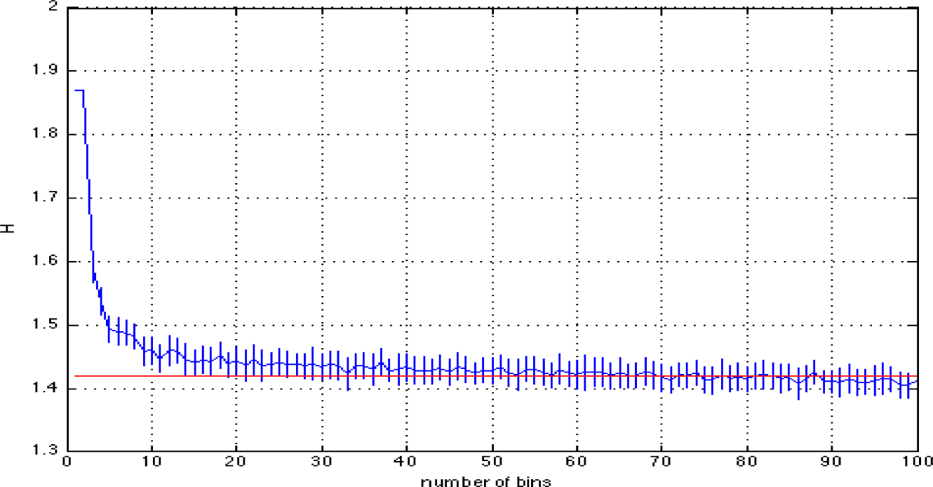
In Figure A.2.2, we illustrate the entropy estimates for this data set as a function of the number of bins where the vertical bars denote one standard deviation from the mean.
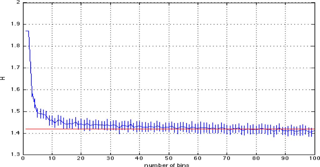
Figure A.2.2.
Entropy estimate of a data-set outside of 76% percentile success rate (for one of the data-sets in the remaining 24% of 100 trials).
Figure A.2.2 shows that the true value of the entropy does not fall into the one standard deviation interval of the mean estimate using Mopt =11, implying that the required number of bins is different for an optimal pdf model and an optimal entropy estimation. It is seen that M = 19 is the smallest number of bins where the entropy estimate falls within this interval and has a very close log p(M|d) value compared to that obtained for M = 11 in Figure A.2.1.b.
Appendix 3
In Appendix 2, we estimated the entropy of a one-dimensional Gaussian variable using the Generalized Knuth method with the prior shown in Equations (8) and (9). We notice that, even in the one-dimensional case, some of the entropy estimates lie outside the confidence intervals. If we estimate the joint entropy of two variables or more, the quality of the estimation decreases further due to empty bins. To overcome this problem, we proposed a different prior Equation (13) and computed the percentages of the relevant entropy estimates falling into 1 and 2 standard deviations (sigma’s) within a total of 100 data-sets sampled from the same two-dimensional Gaussian distribution given by
. Figure. A.3 illustrates these percentages as a function of different β values. Approximately 50% of the time, the marginal entropy estimate falls into the one-sigma interval for β =0.05, and 80% of the time within the two-sigma interval (compare the first and second columns of Figure A.3). As a comparison, the corresponding statistics are approximately 10% for the marginal entropies falling into the one-sigma and 30% for marginal entropies falling into the two-sigma confidence intervals when we use the Krichevsky-Trofinov Dirichlet prior (β =0.5), as in Equation (8) above. It is also observed that in both cases, the confidence interval statistics are lower for the joint entropies, due to the increase of the dimensionality of the space. As a result of this analysis, we observe the largest percentage of getting an entropy estimate within its one-sigma and two-sigma intervals from the true values take place for β = 0.1.
Above, both joint and marginal Shannon entropies of 100 Gaussian-distributed data-sets are estimated using the Generalized Knuth method for the illustrated β values. Subfigures denote the percentage of estimates within one- and two- standard deviations from their analytical values.
PACS Codes: 89.70.Cf; 02.50.-r; 89.70.-a; 05.10.-a; 02.50.Cw
Author Contributions
All authors conceived, designed and evaluated the experiments. Every author contributed to the preparation of the manuscript. All authors have read and approved the final manuscript.
Conflicts of Interest
The authors declare no conflict of interest.
References
- Gourévitch, B.; Eggermont, J.J. Evaluating information transfer between auditory cortical neurons. J. Neurophysiol. 2007, 97, 2533–2543. [Google Scholar]
- Overbey, L.A.; Todd, M.D. Dynamic system change detection using a modification of the transfer entropy. J. Sound Vibr. 2009, 322, 438–453. [Google Scholar]
- Overbey, L.A.; Todd, M.D. Effects of noise on transfer entropy estimation for damage detection. Mech. Syst. Signal Process. 2009, 23, 2178–2191. [Google Scholar]
- Pearl, J. Causality: Models, Reasoning and Inference; MIT Press: Cambridge, MA, USA, 2000; Volume 29. [Google Scholar]
- Hannachi, A.; Jolliffe, I.T.; Stephenson, D.B. Empirical orthogonal functions and related techniques in atmospheric science: A review. Int. J. Climatol. 2007, 27, 1119–1152. [Google Scholar]
- Principe, J.C.; Xu, D.; Fisher, J. Information theoretic learning. Unsuperv. Adapt. Filter. 2000, 1, 265–319. [Google Scholar]
- Schreiber, T. Measuring information transfer. Phys. Rev. Lett. 2000, 85, 461–464. [Google Scholar]
- Granger, C.W. Investigating causal relations by econometric models and cross-spectral methods. Econometrica 1969, 37, 424–438. [Google Scholar]
- Ancona, N.; Marinazzo, D.; Stramaglia, S. Radial basis function approach to nonlinear Granger causality of time series. Phys. Rev. E 2004, 70, 056221. [Google Scholar]
- Hlaváčková-Schindler, K.; Paluš, M.; Vejmelka, M.; Bhattacharya, J. Causality detection based on information-theoretic approaches in time series analysis. Phys. Rep. 2007, 441, 1–46. [Google Scholar]
- Lizier, J.T.; Prokopenko, M. Differentiating information transfer and causal effect. Eur. Phys. J. B 2010, 73, 605–615. [Google Scholar]
- Kleeman, R. Information flow in ensemble weather predictions. J. Atmos. Sci. 2007, 64, 1005–1016. [Google Scholar]
- Liang, X.S.; The, Liang-Kleeman. Information Flow: Theory and Applications. Entropy 2013, 15, 327–360. [Google Scholar] [CrossRef]
- Sabesan, S.; Narayanan, K.; Prasad, A.; Iasemidis, L.D.; Spanias, A.; Tsakalis, K. Information flow in coupled nonlinear systems: Application to the epileptic human brain. Data Mining Biomed. 2007, 7, 483–503. [Google Scholar]
- Majda, A.J.; Harlim, J. Information flow between subspaces of complex dynamical systems. Proc. Natl. Acad. Sci. USA 2007, 104, 9558–9563. [Google Scholar]
- Liang, X.S.; Kleeman, R. Information transfer between dynamical system components. Phys. Rev. Lett. 2005, 95, 244101. [Google Scholar]
- Ruddell, B.L.; Kumar, P. Ecohydrologic process networks: 1. Identification. Water Resour. Res. 2009, 45. [Google Scholar]
- Ruddell, B.L.; Kumar, P. Ecohydrologic process networks: 2. Analysis and characterization. Water Resour. Res. 2009, 45, W03420. [Google Scholar]
- Kaiser, A.; Schreiber, T. Information transfer in continuous processes. Physica D 2002, 166, 43–62. [Google Scholar]
- Knuth, K.H.; Gotera, A.; Curry, C.T.; Huyser, K.A.; Wheeler, K.R.; Rossow, W.B. Revealing relationships among relevant climate variables with information theory, Proceedings of the Earth-Sun System Technology Conference (ESTC 2005), Adelphi, MD, USA, 27–30 June 2005.
- Shannon, C.E.; Weaver, W. The Mathematical Theory of Communication; University of Illinois Press: Urbana-Champaign, IL, USA, 1949. [Google Scholar]
- Knuth, K.H. Optimal data-based binning for histograms. arXiv preprint physics/0605197. This method has been implemented in Matlab and Python. 2006. Available online: http://knuthlab.rit.albany.edu/index.php/Products/Code & http://www.astroml.org/ accessed on 11 January 2015.
- Wolpert, D.H.; Wolf, D.R. Estimating functions of probability distributions from a finite set of samples. Phys. Rev. E 1995, 52, 6841. [Google Scholar]
- Nemenman, I.; Shafee, F. Bialek13, W. Entropy and Inference, Revisited. Adv. Neur. Inf. Process. Syst. 2002, 1, 471. [Google Scholar]
- Prichard, D.; Theiler, J. Generalized redundancies for time series analysis. Physica D 1995, 84, 476–493. [Google Scholar]
- Roulston, M.S. Estimating the errors on measured entropy and mutual information. Physica D 1999, 125, 285–294. [Google Scholar]
- Grassberger, P. Finite sample corrections to entropy and dimension estimates. Phys. Lett. A 1988, 128, 369–373. [Google Scholar]
- Silverman, B.W. Density Estimation for Statistics and Data Analysis; Chapman & Hall/CRC: London, UK, 1986. [Google Scholar]
- Kleeman, R. Information theory and dynamical system predictability. Entropy 1986, 13, 612–649. [Google Scholar]
- Kleeman, R. Measuring dynamical prediction utility using relative entropy. J. Atmos. Sci. 2002, 59, 2057–2072. [Google Scholar]
- Grassberger, P.; Procaccia, I. Characterization of strange attractors. Phys. Rev. Lett. 1983, 50, 346–349. [Google Scholar]
- Grassberger, P.; Procaccia, I. Measuring the strangeness of strange attractors. Physica D 1983, 9, 189–208. [Google Scholar]
- Kantz, H.; Schreiber, T. Nonlinear time Series Analysis; Cambridge University Press: Cambridge, UK, 2003; Volume 7. [Google Scholar]
- Fraser, A.M.; Swinney, H.L. Independent coordinates for strange attractors from mutual information. Phys. Rev. A 1986, 33, 1134. [Google Scholar]
- Darbellay, G.A.; Vajda, I. Estimation of the information by an adaptive partitioning of the observation space. IEEE Trans. Inf. Theory 1999, 45, 1315–1321. [Google Scholar]
- Kraskov, A.; Stögbauer, H.; Grassberger, P. Estimating mutual information. Phys. Rev. E 2004, 69, 066138. [Google Scholar]
- Gomez-Herrero, G.; Wu, W.; Rutanen, K.; Soriano, M.C.; Pipa, G.; Vicente, R. Assessing coupling dynamics from an ensemble of time series 2010, arXiv:1008.0539.
- Vicente, R.; Wibral, M.; Lindner, M.; Pipa, G. Transfer entropy-a model-free measure of effective connectivity for the neurosciences. J. Comput. Neurosci. 2011, 30, 45–67. [Google Scholar]
- Wibral, M.; Pampu, N.; Priesemann, V.; Siebenhühner, F.; Seiwert, H.; Lindner, M.; Lizier, J.T.; Vicente, R. Measuring Information-Transfer Delays. PLoS One 2013, 8. [Google Scholar] [CrossRef]
- Steeg, G.; Galstyan, V.A. Information-theoretic measures of influence based on content dynamics, Proceedings of the Sixth ACM International Conference on Web Search and Data Mining, Rome, Italy, 4–8 February 2013; pp. 3–12.
- Lorenz, E.N. Deterministic nonperiodic flow. J. Atmos. Sci. 1963, 20, 130–141. [Google Scholar]
- Cover, T.M.; Thomas, J.A. Elements of Information Theory; Wiley: Hoboken, NJ, USA, 2012. [Google Scholar]
- Lizier, J.T.; Prokopenko, M.; Zomaya, A. Local information transfer as a spatiotemporal filter for complex systems. Phys. Rev. E 2008, 77, 026110. [Google Scholar]
- Williams, P.L.; Beer, R.D. Generalized Measures of Information Transfer. 2011, arXiv:1102.1507. Available online: http://arxiv.org/abs/1102.1507 accessed on 9 January 2014.
- Scott, D.W. On optimal and data-based histograms. Biometrika 1979, 66, 605–610. [Google Scholar]
- Freedman, D.; Diaconis, P. On the histogram as a density estimator: L 2 theory. Probab. Theory Relat. Fields 1981, 57, 453–476. [Google Scholar]
- Box, G.E.; Tiao, G.C. Bayesian Inference in Statistical Analysis; No. 622; Addison-Wesley: Boston, MA, USA, 1973. [Google Scholar]
- Cellucci, C.J.; Albano, A.M.; Rapp, P.E. Statistical validation of mutual information calculations: Comparison of alternative numerical algorithms. Phys. Rev. E 2005, 71, 066208. [Google Scholar]
- Kugiumtzis, D. Improvement of Symbolic Transfer Entropy, Proceedings of the 3rd International Conference on Complex Systems and Applications, Le Havre, France, 29 June–2 July 2009; Bertelle, C., Liu, X., Aziz-Alaoui, M.A., Eds.; pp. 338–342.
- Prokopenko, M.; Lizier, J.T. Transfer Entropy and Transient Limits of Computation. Sci. Rep. 2014, 4, 5394. [Google Scholar] [CrossRef]
- Lungarella, M.; Ishiguro, K.; Kuniyoshi, Y.; Otsu, N. Methods for quantifying the causal structure of bivariate time series. Int. J. Bifurc. Chaos 2007, 17, 903–921. [Google Scholar]
- Grassberger, P. Grassberger-Procaccia algorithm. Scholarpedia 2007, 2, 3043. [Google Scholar] [CrossRef]
- Dionisio, A.; Menezes, R.; Mendes, D.A. Mutual information: A measure of dependency for nonlinear time series. Physica A 2004, 344, 326–329. [Google Scholar]
- Moddemeijer, R. On estimation of entropy and mutual information of continuous distributions. Signal Process. 1989, 16, 233–248. [Google Scholar]
- Staniek, M.; Lehnertz, K. Symbolic Transfer Entropy. Phys. Rev. Lett. 2008, 100, 158101. [Google Scholar]
- Abramowitz, M.; Stegun, I. Handbook of Mathematical Functions; Dover Publications: New York, NY, USA, 1972. [Google Scholar]
© 2015 by the authors; licensee MDPI, Basel, Switzerland This article is an open access article distributed under the terms and conditions of the Creative Commons Attribution license (http://creativecommons.org/licenses/by/4.0/).


