
Approximate Methods for Maximum Likelihood Estimation of Multivariate Nonlinear Mixed-Effects Models

Abstract
:1. Introduction
2. Five Approximate ML Procedures
2.1. PNLS-MLME Procedure
2.2. Laplacian Procedure
2.3. Pseudo-ECM Algorithm
- E step:
- Evaluate the expected complete-data log-likelihood Function Equation (16) conditioning on the current estimates and the pseudo-responses , which linearize the regression function around the previous estimates of mixed effects and should be updated at each iteration. This gives rise to the so-called Q-function:where:with , , and , where represents the updated pseudo-responses.
- CM step:
- Update the current estimates , , and by maximizing the Q-functionEquation (17). We obtain:where is an matrix consisting of the -th to the -th columns and rows of in which β and D have been replaced by their updated estimates at the iteration. Besides, in the above optimization function for is evaluated at , except for ϕ.
2.4. Monte Carlo EM Algorithm
2.5. Importance Sampling EM Algorithm
2.6. Expected Information Matrix
2.7. Initialization
- (i)
- A direct way of obtaining the initial value for β is to fit the NLMMs to each outcome variable separately by using the nlme R package [12].
- (ii)
- Using the fitting results of NLMMs for each outcome, we take the initial value as a (block) diagonal form with the diagonal entry being the variances (covariances) of random effects under the fitted NLMMs.
- (iii)
- For the initial value for ∑, we use the sample variance-covariance matrix of the data. That is, take , where and .
- (iv)
- The initial values for ϕ, depending on the structure, are simply chosen to give a condition of nearly uncorrelated errors.
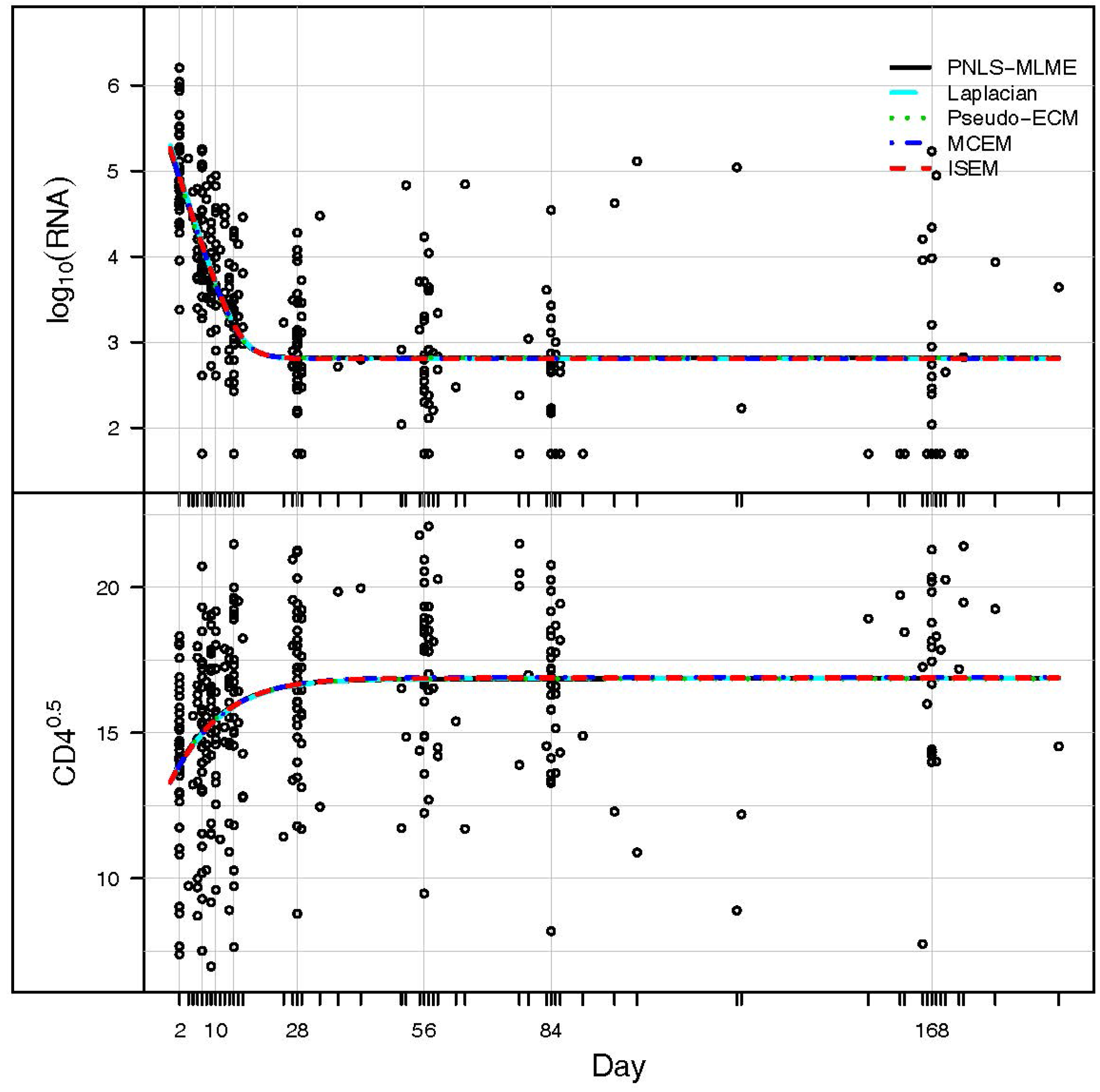
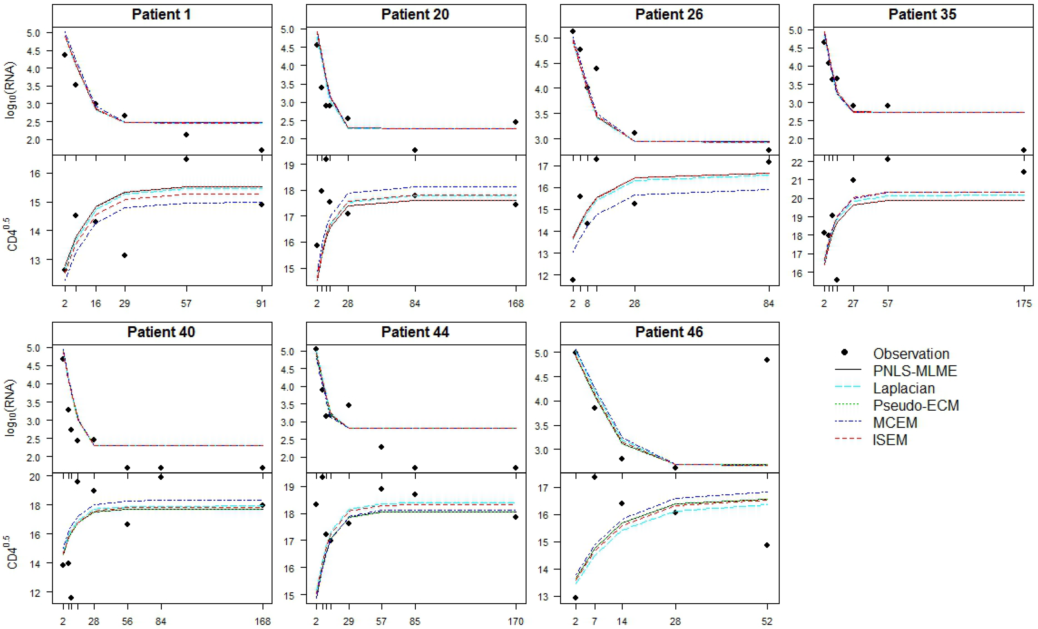
3. Application: ACTG 315 Data


| Parameter | PNLS-MLME | Laplacian | Pseudo-ECM | MCEM | ISEM |
|---|---|---|---|---|---|
| β1 | 12.0477 | 12.9800 | 12.0485 | 12.0784 | 12.114 |
| (0.2513) | (0.2858) | (0.2530) | (0.2626) | (0.2652) | |
| β2 | −2.6558 | −2.6476 | −2.6543 | −2.6198 | −2.6069 |
| (0.1781) | (0.1970) | (0.1777) | (0.1950) | (0.1992) | |
| β3 | 1.3039 | 1.3001 | 1.3039 | 1.3012 | 1.3000 |
| (0.0274) | (0.0248) | (0.0273) | (0.0253) | (0.0249) | |
| β4 | 16.8604 | 16.8577 | 16.8605 | 16.8875 | 16.9058 |
| (0.3911) | (0.3340) | (0.3914) | (0.3863) | (0.3829) | |
| β5 | −1.7324 | −1.7791 | −1.7312 | −1.7721 | −1.7643 |
| (0.4936) | (0.4590) | (0.4930) | (0.4632) | (0.4585) | |
| β6 | 1.3081 | 1.3514 | 1.3078 | 1.3604 | 1.3463 |
| (0.3262) | (0.2899) | (0.3259) | (0.2972) | (0.2896) | |
| 0.0000 | 0.7457 | 0.0583 | 0.1183 | 0.1398 | |
| (0.4665) | (0.5763) | (0.4753) | (0.4673) | (0.4612) | |
| −0.0020 | −0.1400 | 0.0144 | −0.2386 | 0.0838 | |
| (0.5414) | (0.5203) | (0.5479) | (0.5401) | (0.5295) | |
| 4.7425 | 3.8251 | 4.7585 | 5.4602 | 5.4894 | |
| (1.3803) | (0.9953) | (1.3826) | (1.3561) | (1.3361) | |
| σ11 | 0.4655 | 0.4267 | 0.4622 | 0.4379 | 0.4329 |
| (0.0458) | (0.0411) | (0.0455) | (0.0420) | (0.0414) | |
| σ21 | −0.2232 | −0.1738 | −0.2164 | −0.2185 | −0.2225 |
| (0.0965) | (0.0747) | (0.0962) | (0.0786) | (0.0754) | |
| σ22 | 5.7063 | 3.5558 | 5.6929 | 3.8956 | 3.6033 |
| (0.5991) | (0.3520) | (0.5980) | (0.3874) | (0.3541) | |
| ϕ | 0.6824 | 0.5447 | 0.6818 | 0.5674 | 0.5343 |
| (0.0311) | (0.0422) | (0.0312) | (0.0400) | (0.0425) |
| PNLS-MLME | Laplacian | Pseudo-ECM | MCEM | ISEM | |
|---|---|---|---|---|---|
| Approximate | −974.360 | −986.794 | −974.592 | −966.763 | −1010.370 |
| Exact | −1063.338 | −991.754 | −978.269 | −981.384 | −978.758 |
| AD | 88.978 | 4.96 | 3.677 | 14.621 | 31.612 |
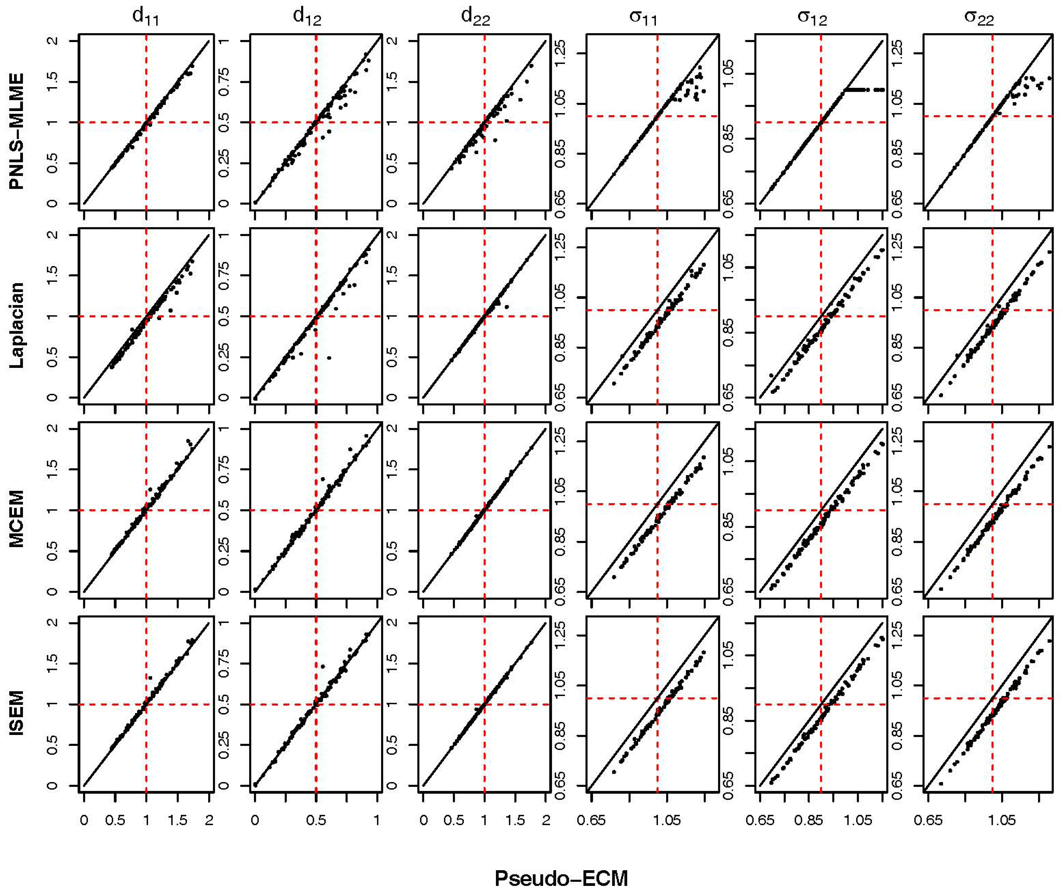
4. Simulation Study
4.1. Bivariate Linear Case
| N | ρ | PNLS-MLME | Laplacian | Pseudo-ECM | MCEM | ISEM | |
|---|---|---|---|---|---|---|---|
| 25 | 0 | Time | 4.077 | 25.954 | 1.970 | 8789.093 | 5862.499 |
| Iter | 2.150 | 12.140 | 9.800 | 138.440 | 58.390 | ||
| −576.769 | −610.274 | −577.121 | −556.914 | −642.139 | |||
| RB | 0.008 | −0.033 | 0.008 | 0.045 | −0.100 | ||
| RMSE | 2.229 | 2.441 | 2.169 | 2.176 | 2.177 | ||
| 0.5 | Time | 4.370 | 30.803 | 2.045 | 2403.145 | 1680.319 | |
| Iter | 2.120 | 11.430 | 9.930 | 35.650 | 15.750 | ||
| −559.366 | −582.622 | −559.907 | −536.608 | −625.736 | |||
| RB | 0.009 | −0.022 | 0.008 | 0.052 | −0.103 | ||
| RMSE | 0.580 | 0.672 | 0.561 | 0.601 | 0.602 | ||
| 0.9 | Time | 3.646 | 25.006 | 1.749 | 1252.625 | 1158.028 | |
| Iter | 2.000 | 8.940 | 8.570 | 18.330 | 10.760 | ||
| −468.270 | −474.786 | −468.909 | −423.555 | −535.591 | |||
| RB | 0.011 | −0.003 | 0.009 | 0.118 | −0.120 | ||
| RMSE | 0.470 | 0.484 | 0.450 | 0.486 | 0.477 | ||
| 50 | 0 | Time | 8.365 | 41.545 | 8.927 | 6825.341 | 3967.824 |
| Iter | 2.240 | 10.050 | 9.260 | 56.240 | 20.170 | ||
| −1159.337 | −1177.863 | −1159.675 | −1120.721 | −1292.848 | |||
| RB | 0.004 | −0.010 | 0.004 | 0.039 | −0.094 | ||
| RMSE | 1.688 | 1.747 | 1.685 | 1.692 | 1.689 | ||
| 0.5 | Time | 9.776 | 56.560 | 10.210 | 2112.857 | 1706.392 | |
| Iter | 2.140 | 9.760 | 9.530 | 11.800 | 9.690 | ||
| −1124.354 | −1140.195 | −1124.911 | −1079.401 | −1258.644 | |||
| RB | 0.004 | −0.009 | 0.004 | 0.046 | −0.098 | ||
| RMSE | 0.277 | 0.324 | 0.270 | 0.313 | 0.315 | ||
| 0.9 | Time | 8.185 | 34.382 | 6.666 | 1512.85 | 1091.661 | |
| Iter | 2.000 | 6.070 | 6.210 | 7.320 | 6.850 | ||
| −933.662 | −943.973 | −934.566 | −843.025 | −1069.55 | |||
| RB | 0.005 | −0.006 | 0.004 | 0.113 | −0.116 | ||
| RMSE | 0.226 | 0.229 | 0.226 | 0.237 | 0.234 |


4.2. Bivariate Nonlinear Case
| Sample Size N | Methods | Comparison Criteria | ||||
|---|---|---|---|---|---|---|
| Time | Iter | RB | RMSE | |||
| 25 | PNLS-MLME | 5.071 | 3.533 | −847.968 | 0.009 | 1.671 |
| Laplacian | 21.199 | 7.133 | −860.383 | −0.012 | 2.000 | |
| Pseudo-ECM | 2.709 | 12.000 | −847.994 | 0.009 | 1.967 | |
| MCEM | 9062.743 | 380.000 | −847.217 | 0.010 | 2.099 | |
| MCEM | 9569.619 | 213.733 | −847.346 | 0.010 | 2.072 | |
| MCEM | 11,375.297 | 131.400 | −847.896 | 0.009 | 2.029 | |
| ISEM | 17,008.449 | 333.733 | −887.996 | −0.028 | 1.999 | |
| ISEM | 4635.601 | 93.400 | −881.169 | −0.018 | 1.882 | |
| ISEM | 1086.651 | 22.200 | −862.842 | −0.020 | 2.077 | |
| 50 | PNLS-MLME | 14.149 | 3.940 | −1710.123 | 0.007 | 1.119 |
| Laplacian | 53.066 | 7.690 | −1763.046 | −0.010 | 1.134 | |
| Pseudo-ECM | 11.331 | 13.070 | −1710.216 | 0.007 | 1.110 | |
| MCEM | 15,860.866 | 392.595 | −1713.939 | 0.005 | 1.184 | |
| MCEM | 24,077.335 | 238.470 | −1714.151 | 0.005 | 1.157 | |
| MCEM | 26,328.930 | 134.750 | −1714.447 | 0.004 | 1.151 | |
| ISEM | 31,224.663 | 386.120 | −1789.168 | −0.021 | 1.255 | |
| ISEM | 7065.363 | 106.350 | −1780.396 | −0.015 | 1.138 | |
| ISEM | 2805.677 | 26.870 | −1779.298 | −0.018 | 1.153 | |
| Sample Size N | Methods | Parameter | |||||||||||
|---|---|---|---|---|---|---|---|---|---|---|---|---|---|
| 25 | PNLS-MLME | 0.046 | 0.960 | 0.046 | 0.041 | 18.505 | 11.559 | 21.698 | 87.774 | 4.565 | 0.998 | 20.003 | 0.909 |
| Laplacian | 0.045 | 0.965 | 0.046 | 0.033 | 18.600 | 11.766 | 20.875 | 120.340 | 4.609 | 1.412 | 20.013 | 1.325 | |
| Pseudo-ECM | 0.043 | 0.964 | 0.046 | 0.026 | 18.501 | 11.570 | 20.066 | 118.786 | 4.759 | 0.988 | 20.010 | 0.909 | |
| MCEM | 0.046 | 0.956 | 0.045 | 0.039 | 18.736 | 11.781 | 20.926 | 130.477 | 4.549 | 1.389 | 19.682 | 1.299 | |
| MCEM | 0.047 | 0.969 | 0.045 | 0.038 | 18.589 | 11.668 | 21.160 | 127.668 | 4.797 | 1.383 | 19.559 | 1.314 | |
| MCEM | 0.047 | 0.970 | 0.046 | 0.036 | 18.602 | 11.669 | 20.402 | 123.817 | 4.606 | 1.404 | 19.935 | 1.315 | |
| ISEM | 0.046 | 0.960 | 0.046 | 0.028 | 18.590 | 11.666 | 20.510 | 120.740 | 4.609 | 1.400 | 20.013 | 1.315 | |
| ISEM | 0.047 | 0.969 | 0.046 | 0.040 | 18.420 | 11.476 | 19.930 | 110.919 | 4.000 | 1.463 | 19.619 | 1.271 | |
| ISEM | 0.043 | 0.993 | 0.045 | 0.021 | 18.785 | 11.899 | 26.451 | 122.587 | 4.407 | 1.631 | 19.474 | 1.377 | |
| 50 | PNLS-MLME | 0.053 | 0.433 | 0.019 | 0.083 | 8.038 | 6.437 | 9.609 | 62.998 | 3.126 | 0.355 | 20.445 | 0.290 |
| Laplacian | 0.054 | 0.433 | 0.019 | 0.040 | 8.056 | 6.501 | 10.172 | 63.165 | 3.121 | 0.787 | 20.025 | 1.051 | |
| Pseudo-ECM | 0.053 | 0.432 | 0.019 | 0.043 | 8.055 | 6.452 | 8.858 | 62.921 | 3.013 | 0.355 | 20.493 | 0.289 | |
| MCEM | 0.052 | 0.420 | 0.019 | 0.087 | 8.117 | 6.505 | 10.334 | 67.836 | 3.055 | 0.875 | 20.054 | 1.033 | |
| MCEM | 0.054 | 0.420 | 0.019 | 0.085 | 8.149 | 6.508 | 10.099 | 65.263 | 3.113 | 0.881 | 20.003 | 1.063 | |
| MCEM | 0.054 | 0.418 | 0.019 | 0.075 | 8.120 | 6.494 | 10.185 | 64.350 | 3.120 | 0.892 | 20.274 | 1.070 | |
| ISEM | 0.059 | 0.415 | 0.019 | 0.080 | 8.034 | 6.429 | 18.313 | 67.054 | 3.142 | 0.924 | 20.045 | 1.011 | |
| ISEM | 0.055 | 0.429 | 0.019 | 0.053 | 8.131 | 6.508 | 9.040 | 64.614 | 3.143 | 0.861 | 19.819 | 1.080 | |
| ISEM | 0.052 | 0.431 | 0.019 | 0.035 | 8.194 | 6.554 | 10.182 | 64.165 | 3.011 | 0.987 | 20.542 | 1.147 | |
5. Discussion and Conclusions
Acknowledgments
Conflicts of Interest
Appendix
A. Score Vector and Hessian Matrix
References
- Shah, A.; Laird, N.; Schoenfeld, D. A Random-Effects Model for Multiple Characteristics with Possibly Missing Data. J. Am. Stat. Assoc. 1997, 92, 775–779. [Google Scholar] [CrossRef]
- Marshall, G.; de la Cruz-Mesía, R.; Barón, A.E.; Rutledge, J.H.; Zerbe, G.O. Non-linear Random Effects Model for Multivariate Responses with Missing Data. Statist. Med. 2006, 25, 2817–2830. [Google Scholar] [CrossRef] [PubMed]
- Sammel, M.; Lin, X.; Ryan, L. Multivariate Linear Mixed Models for Multiple Outcomes. Statist. Med. 1999, 18, 2479–2492. [Google Scholar] [CrossRef]
- Song, X.; Davidian, M.; Tsiatis, A.A. An Estimator for the Proportional Hazards Model with Multiple Longitudinal Covariates Measured with Error. Biostatistics 2002, 3, 511–528. [Google Scholar] [CrossRef] [PubMed]
- Roy, J.; Lin, X. Analysis of Multivariate Longitudinal Outcomes with Nonignorable Dropouts and Missing Covariates: Changes in Methadone Treatment Practices. J. Am. Stat. Assoc. 2002, 97, 40–52. [Google Scholar] [CrossRef]
- Roy, A. Estimating Correlation Coefficient between Two Variables with Repeated Observations Using Mixed Effects Model. Biom. J. 2006, 48, 286–301. [Google Scholar] [CrossRef] [PubMed]
- Wang, W.L.; Fan, T.H. ECM-Based Maximum Likelihood Inference for Multivariate Linear Mixed Models with Autoregressive Errors. Comput. Stat. Data Anal. 2010, 54, 1328–1341. [Google Scholar] [CrossRef]
- Lindstrom, M.J.; Bates, D.M. Nonlinear Mixed Effects Models for Repeated Measures Data. Biometrics 1990, 46, 673–687. [Google Scholar] [CrossRef] [PubMed]
- Davidian, M.; Giltinan, D.M. Nonlinear Models for Repeated Measurements Data; Chapman & Hall: London, UK, 1995. [Google Scholar]
- Pinheiro, J.C.; Bates, D.M. Approximations to the Log-Likelihood Function in the Nonlinear Mixed-Effects Model. J. Comput. Graph. Stat. 1995, 4, 12–35. [Google Scholar]
- Pinheiro, J.C.; Bates, D.M. Mixed-Effects Models in S and S-PLUS; Springer: Berlin, Germany, 2000. [Google Scholar]
- Pinheiro, J.; Bates, D.; DebRoy, S.; Sarkar, D.; R Core Team. nlme: Linear and Nonlinear Mixed Effects Models, R package version 3.1-104; Available online: http://CRAN.R-project.org/package=nlme (accessed on 24 July 2015).
- Dey, D.K.; Chen, M.H.; Chang, H. Bayesian Approach for Nonlinear Random Effects Models. Biometrics 1997, 53, 1239–1252. [Google Scholar] [CrossRef]
- Huang, Y.; Liu, D.; Wu, H. Hierarchical Bayesian Methods for Estimation of Parameters in a Longitudinal HIV Dynamic System. Biometrics 2006, 62, 413–423. [Google Scholar] [CrossRef] [PubMed]
- Lachosa, V.H.; Castrob, L.M.; Dey, D.K. Bayesian Inference in Nonlinear Mixed-Effects Models Using Normal Independent Distributions. Comput. Stat. Data Anal. 2013, 64, 237–252. [Google Scholar] [CrossRef]
- Wolfinger, R.D.; Lin, X. Two Taylor-Series Approximation Methods for Nonlinear Mixed Models. Comput. Stat. Data Anal. 1997, 25, 465–490. [Google Scholar] [CrossRef]
- Ge, Z.; Bickel, J.P.; Rice, A.J. An Approximate Likelihood Approach to Nonlinear Mixed Effects Models via Spline Approximation. Comput. Stat. Data Anal. 2004, 46, 747–776. [Google Scholar] [CrossRef]
- Walker, S.G. An EM Algorithm for Nonlinear Random Effects Models. Biometrics 1996, 52, 934–944. [Google Scholar] [CrossRef]
- Wang, J. EM Algorithms for Nonlinear Mixed Effects Models. Comput. Stat. Data Anal. 2007, 51, 3244–3256. [Google Scholar] [CrossRef]
- Vonesh, E.F.; Wang, H.; Nie, L.; Majumdar, D. Conditional Second-order Generalized Estimating Equations for Generalized Linear and Nonlinear Mixed-Effects Models. J. Am. Stat. Assoc. 2002, 97, 271–283. [Google Scholar] [CrossRef]
- Vonesh, E.F. Non-linear Models for the Analysis of Longitudinal Data. Stat. Med. 1992, 11, 1929–1954. [Google Scholar] [CrossRef] [PubMed]
- Beal, S.; Sheiner, L. The NONMEM System. Am. Stat. 1980, 34, 118–199. [Google Scholar] [CrossRef]
- Wolfinger, R.D. Comment: Experiences with the SAS Macro NLINMIX. Stat. Med. 1997, 16, 1258–1259. [Google Scholar]
- Wolfinger, R.D. Fitting Nonlinear Mixed Models with the New NLMIXED Procedure. In Proceedings of the 99 Joint Statistical Meetings, Miami Beach, FL, USA, 11–14 April 1999.
- Kuhn, E.; Lavielle, M. Maximum Likelihood Estimation in Nonlinear Mixed Effects Models. Comput. Stat. Data Anal. 2005, 49, 1020–1038. [Google Scholar] [CrossRef]
- Lavielle, M. MONOLIX (MOdelès NOn LInéaires à effets miXtes); MONOLIX Group: Orsay, France, 2008. [Google Scholar]
- Beal, S.; Sheiner, L.; Boeckmann, A.; Bauer, R. NONMEM User's Guides (1989–2009); Icon Development Solutions: Ellicott City, MD, USA, 2009. [Google Scholar]
- Comets, E.; Lavenu, A.; Lavielle, M. Saemix: Stochastic Approximation Expectation Maximization (SAEM) Algorithm. R package version 1. 2011. [Google Scholar]
- Wang, W.L.; Fan, T.H. Estimation in Multivariate t Linear Mixed Models for Multiple Longitudinal Data. Statist. Sinica 2011, 21, 1857–1880. [Google Scholar] [CrossRef]
- Wang, W.L.; Fan, T.H. Bayesian Analysis of Multivariate t Linear Mixed Models Using a Combination of IBF and Gibbs Samplers. J. Multivar. Anal. 2012, 105, 300–310. [Google Scholar] [CrossRef]
- Wang, W.L. Multivariate t Linear Mixed Models for Irregularly Observed Multiple Repeated Measures with Missing Outcomes. Biom. J. 2013, 55, 554–571. [Google Scholar] [CrossRef] [PubMed]
- Tierney, L.; Kadane, J.B. Accurate Approximations for Posterior Moments and Densities. J. Am. Stat. Assoc. 1986, 81, 82–86. [Google Scholar] [CrossRef]
- Meng, X.L.; Rubin, D.B. Maximum Likelihood Estimation via the ECM Algorithm: A General Framework. Biometrika 1993, 80, 267–278. [Google Scholar] [CrossRef]
- Booth, G.J.; Hobert, P.J. Maximizing Generalized Linear Mixed Model Likelihoods with an Automated Monte Carlo EM Algorithm. J. R. Stat. Soc. Ser. B 1999, 61, 265–285. [Google Scholar] [CrossRef]
- Lai, T.L.; Shih, M.C. A Hybrid Estimator in Nonlinear and Generalized Linear Mixed Effects Models. Biometrika 2006, 90, 791–795. [Google Scholar]
- Leonard, T.; Hsu, J.S.J.; Tsui, K.W. Bayesian Marginal Inference. J. Am. Stat. Assoc. 1989, 84, 1051–1058. [Google Scholar] [CrossRef]
- Bates, D.M.; Watts, D.G. Relative Curvature Measures of Nonlinearity. J. R. Stat. Soc. Ser. B 1980, 42, 1–25. [Google Scholar]
- R Development Core Team. R. A Language and Environment for Statistical Computing; R Foundation for Statistical Computing: Vienna, Austria, 2012. [Google Scholar]
- Dempster, A.P.; Laird, N.M.; Rubin, D.B. Maximum Likelihood Estimation from Incomplete Data via the EM Algorithm (with Discussion). J. R. Stat. Soc. Ser. B 1977, 39, 1–38. [Google Scholar]
- Wei, G.C.G.; Tanner, M.A. A Monte Carlo Implementation of the EM Algorithm and the Poor's Man's Data Augmentation Algorithms. J. Am. Stat. Assoc. 1990, 85, 699–704. [Google Scholar] [CrossRef]
- Hastings, W.K. Monte Carlo Sampling Methods Using Markov Chains and Their Applications. Biometrika 1970, 57, 97–109. [Google Scholar] [CrossRef]
- Lederman, M.M.; Connick, E.; Landay, A.; Kuritzkes, D.R.; Spritzler, J.; Clair, M.S.; Kotzin, B.L.; Fox, L.; Chiozzi, M.H.; Leonard, J.M.; et al. Immunologic Responses Associated with 12 Weeks of Combination Antiretroviral Therapy Consisting of Zidovudine, Lamivudine, and Ritonavir: Results of AIDS Clinical Trials Group Protocol 315. J. Infect. Dis. 1998, 178, 70–79. [Google Scholar] [CrossRef] [PubMed]
- Connick, E.; Lederman, M.M.; Kotzin, B.L.; Spritzler, J.; Kuritzkes, D.R.; Clair, M.S.; Sevin, A.D.; Fox, L.; Chiozzi, M.H.; Leonard, J.M.; et al. Immune Reconstitution in the First Year of Potent Antiretroviral Therapy and Its Relationship to Virologic Response. J. Infect. Dis. 2000, 181, 358–363. [Google Scholar] [CrossRef] [PubMed]
- Wu, H.; Ding, A. Population HIV-1 Dynamics in Vivo: Applicable Models and Inferential Tools for Virological Data from AIDS Clinical Trials. Biometrics 1999, 55, 410–418. [Google Scholar] [CrossRef] [PubMed]
- Liang, H.; Wu, H.; Carroll, R.J. The Relationship between Virologic Responses in AIDS Clinical Research Using Mixed-Effects Varying-Coefficient Models with Measurement Error. Biostatistics 2003, 4, 297–312. [Google Scholar] [CrossRef] [PubMed]
- Wu, H.; Liang, H. Backfitting Random Varying-Coefficient Models with Timedependent Smoothing Covariates. Scand. J. Stat. 2004, 31, 3–19. [Google Scholar] [CrossRef]
- Lin, T.I.; Wang, W.L. Multivariate Skew-Normal Linear Mixed Models for Multi-outcome Longitudinal Data. Stat. Model. 2013, 13, 199–221. [Google Scholar] [CrossRef]
- Lin, T.I.; Lee, J.C. A Robust Approach to t Linear Mixed Models Applied to Multiple Sclerosis Data. Statist. Med. 2006, 25, 1397–1412. [Google Scholar] [CrossRef] [PubMed]
- Lin, T.I.; Lee, J.C. Bayesian Analysis of Hierarchical Linear Mixed Modeling Using Multivariate t Distributions. J. Statist. Plan. Inf. 2007, 137, 484–495. [Google Scholar] [CrossRef]
- Lin, T.I.; Lee, J.C. Estimation and Prediction in Linear Mixed Models with Skew Normal Random Effects for Longitudinal Data. Statist. Med. 2008, 27, 1490–1507. [Google Scholar] [CrossRef] [PubMed]
- Arellano-Valle, R.B.; Genton, M. On Fundamental Skew Distributions. J. Multivar. Anal. 2005, 96, 93–116. [Google Scholar] [CrossRef]
- Azzalini, A.; Capitaino, A. Distributions Generated by Perturbation of Symmetry with Emphasis on a Multivariate Skew t-Distribution. J. R. Stat. Soc. Ser. B 2003, 65, 367–389. [Google Scholar] [CrossRef]
- Branco, M.; Dey, D. A General Class of Multivariate Skew-Elliptical Distribution. J. Multivar. Anal. 2001, 79, 93–113. [Google Scholar] [CrossRef]
- Bandyopadhyay, D.; Lachos, V.H.; Abanto-Vallec, C.A.; Ghosh, P. Linear Mixed Models for Skew-Normal/Independent Bivariate Responses with an Application to Periodontal Disease. Statist. Med. 2010, 29, 2643–2655. [Google Scholar] [CrossRef] [PubMed]
- Bandyopadhyay, D.; Castro, L.M.; Lachos, V.H.; Pinheiro, H.P. Robust Joint Non-linear Mixed-Effects Models and Diagnostics for Censored HIV Viral Loads with CD4 Measurement Error. J. Agr. Biol. Environ. Stat. 2015, 20, 121–139. [Google Scholar] [CrossRef]
© 2015 by the author; licensee MDPI, Basel, Switzerland. This article is an open access article distributed under the terms and conditions of the Creative Commons Attribution license (http://creativecommons.org/licenses/by/4.0/).
Share and Cite
Wang, W.-L. Approximate Methods for Maximum Likelihood Estimation of Multivariate Nonlinear Mixed-Effects Models. Entropy 2015, 17, 5353-5381. https://doi.org/10.3390/e17085353
Wang W-L. Approximate Methods for Maximum Likelihood Estimation of Multivariate Nonlinear Mixed-Effects Models. Entropy. 2015; 17(8):5353-5381. https://doi.org/10.3390/e17085353
Chicago/Turabian StyleWang, Wan-Lun. 2015. "Approximate Methods for Maximum Likelihood Estimation of Multivariate Nonlinear Mixed-Effects Models" Entropy 17, no. 8: 5353-5381. https://doi.org/10.3390/e17085353
APA StyleWang, W.-L. (2015). Approximate Methods for Maximum Likelihood Estimation of Multivariate Nonlinear Mixed-Effects Models. Entropy, 17(8), 5353-5381. https://doi.org/10.3390/e17085353