Abstract
In this paper, we propose a multiscale dependence-based methodology to analyze the dependence structure and to estimate the downside portfolio risk measures in the energy markets. More specifically, under this methodology, we formulate a new bivariate Empirical Mode Decomposition (EMD) copula based approach to analyze and model the multiscale dependence structure in the energy markets. The proposed model constructs the Copula-based dependence structure formulation in the Bivariate Empirical Mode Decomposition (BEMD)-based multiscale domain. Results from the empirical studies using the typical Australian electricity daily prices show that there exists a multiscale dependence structure between different regional markets across different scales. The proposed model taking into account the multiscale dependence structure demonstrates statistically significantly-improved performance in terms of accuracy and reliability measures.
1. Introduction
The energy markets have been known as one of the most volatile financial markets for a long time, where significant fluctuations have been observed in their production and consumption [1]. Till now, a majority of previous research has focused on modeling and forecasting the physical production and consumption of energy, as well as the movement of the prices determined. Typically employed models include econometric models, artificial intelligence models, etc. [2,3]. However, the observed significant volatility and the risk measurement in the financial energy markets have received much less attention, despite their significant impact on the trading, operation and risk management practice of the energy markets. Accurate measurement of the market price fluctuations and risk level in the energy markets has both theoretical and practical merits [4].
Theoretically, energy market risk measurement represents an important and tough research problem in the field of risk measurement [4]. Firstly, as energy is difficult to store and usually costs too much in storage, it would result in unique price fluctuation patterns and very significant market risk exposure, so that the current market risk measurement methodology no longer suffices. New and innovative market risk measurement models are needed theoretically. For example, since electricity is difficult to store and the price is settled instantaneously, it is a financial asset mostly of a consumption nature and demonstrates a significantly high level of volatility [5]. The extreme and transient events are prevalent in the market with very different behavioral patterns than the other financial markets [6]. The electricity risk measurement needs to be conducted on a much shorter scale and needs to pay particular attention to the finer market structure, especially the impact of the transient and disruptive risk factors on a short-term time horizon [7]. Secondly, market risk measurement is closely related to other important research topics, including volatility forecasting, electricity derivative pricing, portfolio optimization, etc. Value at risk serves as an important ex post measure for the evaluation of the volatility forecasting accuracy, which is a critical parameter for financial derivative pricing.
Practically accurate electricity market risk measurement serves as the foundation for the risk monitoring system and the enterprise risk management system in the electricity related industry. It is a critical factor to consider and control during the operation management and capital budgeting process for any electricity-intensive companies, such as the electric grid, paper manufacturing industry, steel industry, etc. It is also an important risk factor to measure and needs to be integrated into the enterprise-wide risk measure for the cost management and operation management of most manufacturing companies. For example, according to the survey study by KPMG management consulting firm, half of the power plants in Russia pay close attention to the risk measurement, and they usually use value at risk to measure the risk [8].
Over the years, numerous empirical research has conducted the measurement of the market risk in the energy markets. In the long-term time horizon, we have witnessed widespread applications of econometric approaches to model the market volatility, especially considering the spillover effects among different energy markets and other financial markets, in the equilibrium conditions in different energy markets. For example, Chevallier [9] proposes a bivariate model to forecast the density function of West Texas Intermediate (WTI) crude oil future returns. They found that the stochastic jump components contain useful information that needs to be incorporated into the model and could help improve the forecasting accuracy [9]. Barunik et al. [10] analyzed the dynamic asymmetry in the volatility spillover among petroleum markets. They found that there are significant regime changes in volatility asymmetry around both 2001 and 2008 [10]. Lin and Li [11] used the Vector Error Correction-Multivariate Generalized Autoregressive Conditional Heteroskedasticity (VEC-MGARCH) model to identify the spillover between crude oil and gas markets [11]. In the short-term time horizon, the volatility level increases significantly, and its nonlinear dynamic movement becomes more complex. More assumption-free data-driven approaches show the superior performance. Typical examples would be the multi-fractal models, neural network model, etc. Particularly, Youssef et al. [12] used the Fractional Integrated Generalized Autoregressive Conditional Heteroskedasticity (FIGARCH) model to analyze the fractal, long memory and extreme risk characteristics and estimated downside risk measures. They found that the fractal and extreme value-based model would result in the improved risk estimate accuracy in the energy markets [12]. Wang et al. [13] proposed a Markov switching multifractal model to forecast the crude oil volatility at a higher level of accuracy [13]. Bildirici and Ersin [14] introduced the neural network model to augment the nonlinear econometric models and achieved improved crude oil volatility forecasting performance [14].
Although the data-driven approaches have shown that empirical data contain more complex data features that violate the assumptions of most traditional approaches and result in interior performance, what exactly constitute these complex data features remains an open question in the literature. Recently, in the literature, the recognition and modeling of the heterogeneous risk factors, which exhibit drastically different data characteristics, emerged as one alternative approach to explain and model the widely-acknowledged nonlinear risk movements. For example, we would expect the supply and demand risk factors to demonstrate more stationary long-term behaviors. The shocks in some other macroeconomic factors may translate into more short-term stochastic behaviors. This is why current modeling approaches encounter difficulty, because they usually assume that the market is efficient and homogeneous, dominated with one particular data feature only. This assumption may approximate the data over the long-term time horizon. However, for the short and medium time horizons, when the markets do not reach the equilibrium, this assumption is violated. They need to be relaxed further to allow the existence of heterogeneous data features for more accurate modeling of the nonlinear data movement.
When the homogeneous assumption is relaxed, we may assume that the market is dominated with several heterogeneous risk factors. These risk factors are governed by different underlying Data Generating Processes (DGPs). Some well-known data features include autocorrelation, volatility clustering, etc. The multivariate time series models have been proposed to model the multivariate autocorrelation in the mean and correlations and volatility clustering data characteristics in practice. Typical models include the multivariate Autoregressive Moving Average (ARMA) models and multivariate GARCH models. Recently, the non-normal dependence structure among financial portfolio and the multiscale data characteristics are two recent emerging data features that have attracted much research attention. They also give rise to some promising methodologies to deal with the complex data features.
With the heterogeneous data structure in the practical data, the selection and integration of appropriate models capturing different DGPs is an important research problem. The key research issue is to explore a new methodology to integrate different models to capture different components of data. Traditionally, ensemble models in the literature adopting linear or artificial intelligence models have been widely used. For example, Alamaniotis et al. [15] proposed a genetic algorithm that combined relevance vector machines and linear regression models. They applied it in electricity price forecasting and achieved improved forecasting accuracy, comparing to the traditional ARMA model [15]. However, traditional ensemble model assumed that models are independently capturing data characteristics. This integrates different models ex post, where significant estimate bias resulting from the violation of the assumptions of different models is accumulated. Recently, an alternative ex ante approach emerged, under different names, such as divide and conquer, decomposition, etc. For example, Yu et al. [16] purposed the divide and conquer principle to construct a data characteristics-driven decomposition ensemble methodology. The application of this methodology in the crude oil price forecasting showed improved performance [16]. Yu et al. [17] proposed a decomposition and ensemble learning paradigm for crude oil price forecasting [17]. The key to all of these approaches is to separate data components with unique data characteristics ex ante and to select models with the data-matching assumption. Then, the chosen models are integrated together, with lower biases and higher forecasting accuracy. However, current approaches are mainly ad hoc. We argue that different scales in the data could be used as the criteria of separation, so that different models can be used to model different data features. Thus, we propose a new multiscale methodology to estimate value at risk for high dimensional portfolio assets. Following this methodology, we propose the BEMD-copula-based model to demonstrate the effectiveness of the model in capturing the multiscale dependence structure in the data. We also propose to use entropy as the criteria to determine the parameters for BEMD-copula model. Empirical studies using the Australian electricity data as a typical example show that there exists a dynamic time varying dependence structure between New South Wales (NSW) and Queensland (QLD) markets. We show that the proposed model incorporating the multiscale dependence structure tracks the risk evolutions more closely and achieves statistically significant performance improvement in risk measurement accuracy and reliability. This lends further support to the effectiveness of our proposed methodology.
Work in this paper contributes to the literature in the following aspects. Firstly, a new multiscale methodology has been proposed to analyze the multiscale characteristics of risk movement and co-movement. For the proposed methodology, we have identified some important research problems, including the choice of models and the determination of model parameters. Secondly we have proposed a BEMD-copula model under the proposed methodology. We have proposed the alternative entropy-based approach to tackle these research problems. We show that there are different constituent portfolio components with a multiscale structure characterized by different copula functions. The mixture of time varying dependence structure is revealed and explicitly modeled in the BEMD transformed domain. We have confirmed in the empirical studies that the proposed model provides the most accurate characterization of the empirical data. More importantly, with the proposed model, we address explicitly the determination of the multiscale model specifications. We found that the dependence structure is time varying in both the model specifications and parameters across different time scale. During the model fitting process, we found that the entropy measure serves as a better measure to determine the BEMD decomposed multiscale structure.
The rest of the paper proceeds as follows. In Section 2, we present the comprehensive review on the multiscale analysis in the energy markets, as well as the copula model in the energy markets. In Section 3, we propose and illustrate the multiscale methodology for the Portfolio Value at Risk (PVaR) estimate. We also illustrate in detail the numerical algorithm of the BEMD-copula-based model. In Section 4, we report and analyze in detail the original results from experiments conducted using the Australian electricity market data. Section 5 provides some summarizing remarks about the main results, contributions and implications of the work in this paper.
2. Literature Review
2.1. Multiscale Analysis in the Energy Markets
In the literature, multiscale analysis techniques, such as wavelet analysis and empirical mode decomposing, have received considerable research attention as effective techniques to analyze the energy commodity market co-movement. For example, Vacha and Barunik [18] used wavelet coherence analysis to investigate and confirm the existence of the multiscale co-movement among crude oil, natural gas, gasoline and heating oil energy markets [18]. Ortas and Alvarez [19] used the wavelet coherent analysis to identify the lead lag relationship between carbon assets and other energy commodities [19]. Jammazi [20] analyzes the multiscale co-movement relationship between crude oil and stock returns in the Haar a trous wavelet-transformed time scale domain. It is found that the multiscale co-movement is more significant in the higher scale [20]. However, as far as the energy forecasting and risk measurement are concerned, multiscale techniques have received much less attention. In the electricity markets, Rana and Koprinska [21] used wavelet analysis to extract data features at different scales to improve the neural network forecasting accuracy in the Australian electricity market Rana and Koprinska [21]. Voronin and Partanen [22] used wavelet analysis as the feature extraction tool for the follow-up forecasting using Autoregressive Integrated Moving Average (ARIMA) and the neural network model. Empirical studies in the Nordic Power Pool have shown the improved electricity demand and price forecasting accuracy [22]. Shrivastava and Panigrahi [23] used the wavelet analysis as a preprocessor to improve the forecasting accuracy of the extreme learning machine in the Ontario and PJM electricity market [23]. Nguyen and Nabney [24] showed that the combination of wavelet analysis and the neural network model would result in the improved electricity demand and natural gas forecasting accuracy [24]. Jin and Kim [25] forecasted the natural gas price using the combination of wavelet analysis and the neural network [25]. He et al. [26] proposed a wavelet decomposed ensemble model for the crude oil market and found the improved performance of the proposed algorithm against the benchmark models [26]. Zhu et al. [27] proposed the morphological component analysis-based forecasting model and found improved forecasting accuracy in the crude oil markets [27]. Li et al. [28] proposed a wavelet denoising ARMA model ensembled by least square support vector regression. The ensembled crude oil forecasts in the multiscale domain showed improved forecasting accuracy [28]. He et al. [29] proposed a new multivariate wavelet denoising-based approach for estimating PVaR. Empirical studies suggest that the proposed algorithm outperforms the benchmark Exponential Weighted Moving Average (EWMA) and Dynamic Conditional Correlation-Generalized Autoregressive Conditional Heteroskedasticity (DCC-GARCH) model [29]. He et al. [30] proposed a wavelet decomposed-based nonlinear ensemble algorithm, based on artificial neural networks, to estimate Value at Risk (VaR) with higher reliability and accuracy in the crude oil markets [30]. He et al. [31] proposed an Morphological Component Analysis (MCA)-based hybrid methodology for analyzing and forecasting the risk evolution in the crude oil market. MCA is used to extract and analyze the underlying transient data components. Empirical studies show that this approach improves the reliability and stability of VaR estimation [31]. As for the empirical studies using EMD in the energy markets, Zhang et al. [32] combined the ensemble empirical mode decomposition model with the least square support vector regression model. They found that this hybrid approach led to improved forecasting accuracy [32]. Zhu [33] combined the EMD, genetic algorithm and the artificial neural network to forecast more accurate carbon price movement [33]. Yu et al. [34,35] proposed a series of multi-scale neural network ensemble forecasting models based on the EMD model and applied them to the crude oil forecasting exercise [34,35].
2.2. Copula Model in the Energy Markets
When modeling the dependence structure in higher dimensions, dependence modeling extends beyond the correlations between multiple assets in the traditional elliptical multivariate distribution framework. In the literature, it has mainly been used to characterize the dependence structure among portfolio assets in both unconditional and conditional cases. For example, in the unconditional case, Jaschke [36] analyzed the dependence structure between WTI and Brent markets using different copula models. The comprehensive performance valuation on different copula-based risk estimates showed that Gumbel copula provided the best model fitting [36]. Work by Anne-Laure Delatte [37] also showed that the dependence structure between the commodity and the stock markets was predominantly symmetric, as described by the Gaussian copula model [37]. In the conditional case, work by Chih-Chiang Wu [38] showed that the Gaussian copula model provided the best modeling of the conditional dependence structure between the crude oil and the exchange rate [38]. Reboredo [39] found a consistent level of crude oil market linkage, modeled by the copula method in different business cycles, and confirmed the one great pool hypothesis [39]. Chang [40] proposed the mixture copula GARCH model consisting of both Gumbel and Clayton copula to model the asymmetric tail dependence in the crude oil spot and futures markets [40]. Recently, the conditional copula theory has been used to estimate VaR and Portfolio VaR. Huang et al. [41] proposed a Copula Glosten-Jagannathan-Runkle (GJR) GARCH model to estimate value at risk and found it was a more optimal risk measure than traditional variance covariance and Monte Carlo-based approaches [41]. Yan Fang [42] proposed the extended double asymmetric copula GARCH model to account for the asymmetric effects of positive and negative shocks individually. Empirical studies showed that the proposed Dynamic Double Asymmetric Copula (DDAC)-GARCH copula model provided more optimal risk coverage in terms of the value at risk measure [42]. Karl Friedrich Siburg [43] proposed a non-parametric copula-based model to estimate the portfolio value at risk better. The lower tail dependence was estimated non-parametrically, while the dependence specification was estimated using the canonical maximum likelihood method [43]. Ignatieva and Truck [44] analyzed the dependence structure in the electricity markets using different copula models and found the Student t copula provided better dependence structure modeling accuracy and VaR estimation accuracy [44]. Boubaker and Sghaier [45] identifies the long memory feature in the financial returns dependence structure captured using the copula model. The portfolio risk is better captured using the copula-based approach. This empirical evidence has provided the preliminary evidence of positive and improved performance with these methods, which shows the promising products of these methods in the risk measurement literature [45].
However, we have not identified very inter-disciplinary research crossing the multiscale analysis literature and dependence modeling literature. One exception was our initial work on testing the performance of the combination of EMD and the copula model by Wang et al. [46]. Although the initial research has demonstrated that the EMD-based copula may lead to improved performance in the value at risk estimate, in the case of the multivariate forecasting model, the multiscale analysis and modeling of the dependence structure among the individual assets, including both the model identification and forecasting model, has remained an open question in the literature [47]. The main obstacle is the identification and determination of parameters that characterize the multiscale structure among individual assets. This research problem would translate to the identification of edge singularities in the two dimensions and geometric multiscale data features in the higher dimensions.
3. A Multiscale Dependence-Based Methodology for Portfolio Value at Risk Estimate
PVaR is defined as the threshold downside risk statistics measuring the maximal level of losses on the portfolio under the normal market conditions, at the given confidence level and investment time horizon [48]. As far as statistics is concerned, PVaR is mostly concerned with the estimation of the particular quantile of the empirical distribution. The prevailing methods to estimate VaR in the literature mainly include parametric, non-parametric and semi-parametric approaches [48]. The parametric approach goes to one extreme by imposing very strict assumptions in deriving the analytical solutions. Riskmetrics’ Multivariate Exponential Weighted Moving Average (MEWMA) and DCC-GARCH models are two typical approaches [49]. The non-parametric approach goes to the other extreme by imposing the least amount of assumptions and taking data-driven approaches. The ideal model should impose more realistic assumptions and have a high level of traceability. Thus, in recent years, new methodologies with more relaxed assumptions have emerged. They are usually classified as semi-parametric approaches and may include copula theory, Extreme Value Theory (EVT) and signal processing techniques, such as Fourier analysis, wavelet analysis, the EMD algorithm, etc. [34].
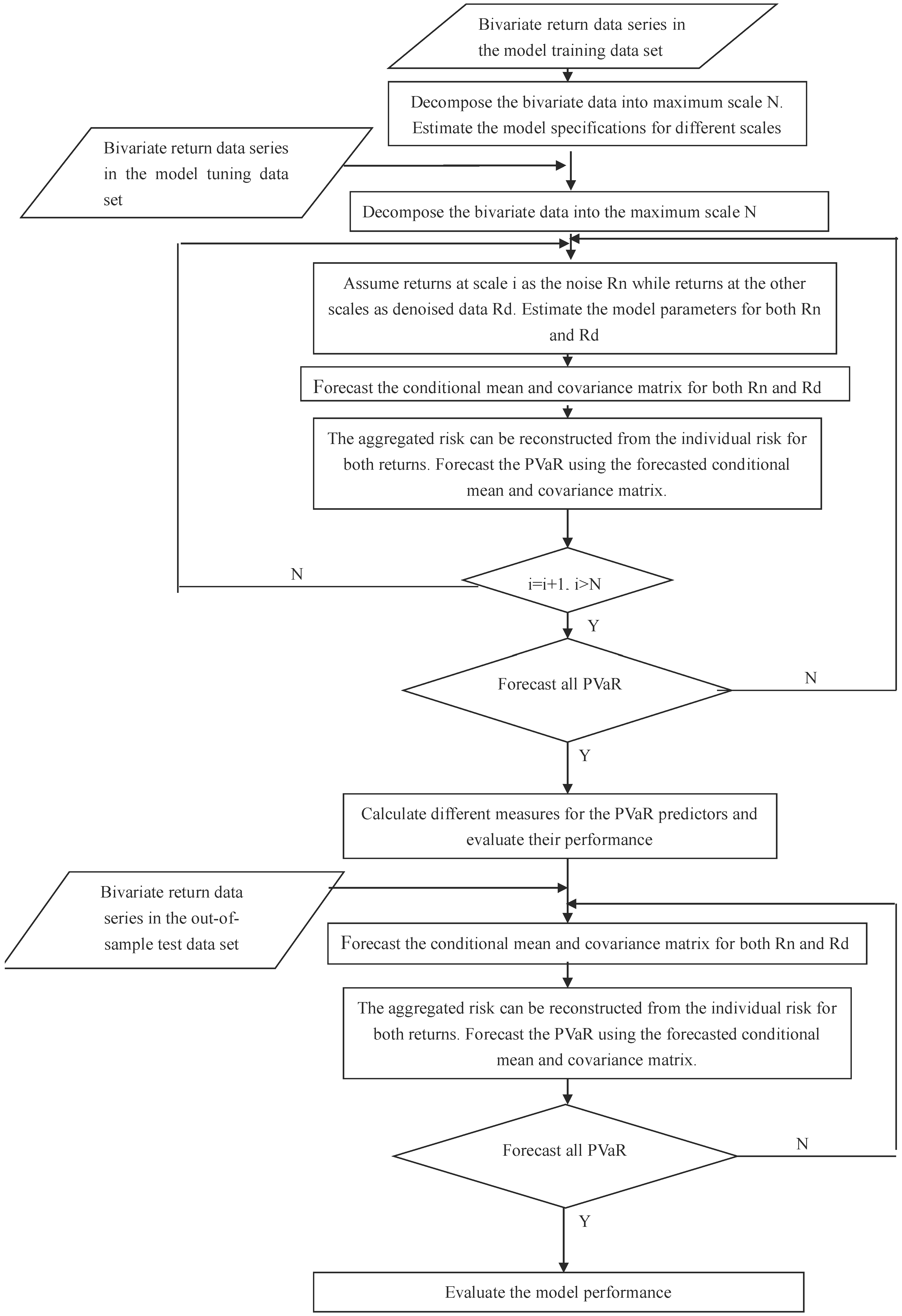
Given the diverse range of data features available, we propose an integrated methodology that takes a decomposition-based multiscale approach to estimate the PVaR of the empirical data distribution. We assume that the data are generated with different DGPs. In the proposed model, we assume that different DGPs are distinguished from one another with different time frequency characteristics. This would imply a one-to-one correspondence between the time scales and frequency scales. One implication of the assumption in the case of risk assessment is that volatilities are independent and heterogeneous, while volatilities are homogeneous within scales. Thus, with the chosen basis functions, the time scale can be used to project the original data into the time scale domain and to separate different DGPs. In the multiscale approach, there are different model specifications and parameters employed across different time scales, to capture different frequency information. Some typical multiscale models used would include the recent emergence of Empirical Model Decomposition (EMD), wavelet analysis, etc. Multiscale theory can be used to empirically derive the constituent data components at different scales, given that the constituent data components are separable and distinguishable by their different speeds of oscillation and the size of fluctuation. The methodology is illustrated as in Figure 1.

Figure 1.
A multiscale integrated Portfolio Value at Risk (PVaR) methodology.
In the first step, in the general case of a portfolio of two assets with returns at time t, a particular multiscale model is used to project the given multivariate energy data series simultaneously into the multiscale domain up to scale N, as in Equation (1).
where and refer to the original return series and the decomposed return series at scale j at time t, respectively. Among them, decomposed data at one scale n are assumed to be the transient data governed by disruptive factors. Data at the rest of the scales are assumed to be the main factors governing the normal data behaviors in the market.
In the second step, using the training data, we fit a series of multivariate models across different scales. More specifically, we estimate the parameters for current multivariate models with different distributions used to fit the energy data in each market individually.
In the third step, we assume that one scale corresponds to the transient data, while the other scales correspond to the normal data. The transient data reflect the market behavior of the transient and disruptive risk factors, while the normal data reflect the joint influences of the normal market risk factors. We assume that the risks of both normal and transient data contribute equally to the overall market risk level. Thus, using the model tuning data, the aggregated variance-covariance estimate is calculated with the equal average of the individual variance-covariance matrix for both normal and transient risk factors as in Equation (2).
where is the aggregated conditional variance-covariance forecast matrix at time t. and are conditional variance-covariance forecast matrices for returns over both normal and transient phenomenon, respectively, at time t. is the covariance matrix at time t, and .
In the fourth step, we estimate PVaR for the model tuning data using the estimated conditional mean matrix and conditional variance-covariance matrix. is estimated as in Equation (3) [48].
where . refers to the variance-covariance matrix. refers to the weight matrix for the portfolio. refers to the relevant quantile from the standard normal distribution. P is the invested portfolio value. h is the holding period. is the threshold at the confidence level .
In the fifth step, assuming that the in-sample PVaR model performance indicates the out-of-sample generalizing PVaR model performance, we adopt different performance measures and decision rules to evaluate the in-sample model performance using the model tuning data. Some typical decision rules and performance measures may include the minimization of the number of exceedances, the maximization of the p-value of the Kupiec backtesting procedure and the minimization of the entropy value.
In the sixth step, with the determined model specifications and parameters, including the optimal scale for the transient factors, we estimate the PVaR for the test dataset. Different performance measures, such as the Kupiec backtesting procedure, are used to evaluate the model performance.
Under the proposed multiscale dependence methodology, we propose a BEMD-copula-based portfolio value at risk model to estimate the portfolio risk assessment. Key to the proposed BEMD-copula PVaR model is the introduction of the BEMD model and copula model, as particular implementations of the proposed methodology.
Firstly, EMD is a recently-emerging signal processing technique to explore, decompose and analyze the underlying data structure, with a multiscale approach. It adaptively extracts the underlying data components, represented as a set of oscillation functions called Intrinsic Mode Functions (IMFs) with different amplitudes and frequency bands, i.e., different fluctuation bands. In the univariate setting, these data characteristics of different amplitudes and frequencies across different scales correspond to different oscillations or fluctuation levels. In the multivariate setting, defining the boundary for different data structures across different scales represents much more difficult research problems. The original concept of univariate oscillations is extended to the rotation in the multivariate case. There are several attempts to define the boundary in the multivariate setting in the literature, including modulated multivariate oscillation models, complex EMD, rotation-invariant EMD and univariate EMD. The bivariate EMD is usually preferred, as it guarantees the same number of IMFs across data channels and is very flexible in the number of projection channels. In the bivariate setting, this provides an important alternative to the traditional multivariate distribution-based analysis to separate the data components with unique characteristics in both their dependence structure and individual patterns, regardless of their particular distributional assumptions.
The BEMD algorithm is illustrated in Algorithm 1.
| Algorithm 1: Bivariate Empirical Mode Decomposition Algorithm |
|
Secondly, the copula theory is also introduced in the proposed BEMD-copula algorithm to model the non-normal dependence structure in the decomposed risk structure, as well as its dependence structure across different scales. In Heterogeneous Market Hypothesis (HMH), the dependence structure across different scales is assumed to be different, exhibiting distinctive frequency characteristics, reflecting different time varying dependence. This demands the use of different copula functions appropriate to characterize the dependence structures at different scales. Then, we can construct the time varying multiscale dependence structure in the BEMD decomposed domain, revealing the heterogeneous time varying risk structure.
When modeling the individual DGPs with the multiscale approach, we assume that the DGPs follow the same model specification, but with different parameters. This implies that different trading strategies are adopted with different parameters. In the proposed model, we introduce the conditional copula model to analyze and model the multivariate conditional distributions. The proposed conditional copula theory extends the original unconditional copula theory to the conditional case, which is of relevance to economics and financial forecasting.
Given some information set w, let be random variables with conditional distribution functions and conditional joint distribution H of , where and W has support ω. The conditional Sklar theorem states that there exits a copula C, such that, for any and , [50].
With the conditional extension of the Sklar theorem, any n dimensional joint distribution can be represented as n dimensional marginal distributions and a dependence function, given that the information set w is consistently used for both the marginal distributions and the copula.
The copula GARCH model is proposed to model the movement dynamics and the dependence structure conditional on the past observations. It is one particular realization of the conditional copula theory, where the random variables X in the marginal distributions are assumed to follow some time series models, such as the ARMA model for the conditional mean and GARCH model for the conditional volatility.
The conditional ARMA-GARCH model following the assumed marginal distributions is defined as in Equation (5).
where and are the conditional mean and conditional variance at time t, respectively. is the lag r returns with parameter , and represents the lag m residuals in the previous period with parameter . is the lag p variance with parameter , and is the lag q squared errors with parameter in the previous period. refers to the selected probability density function of the residuals from the ARMA model, where ϑ refers to the shape parameters for the assumed distribution.
The estimation of the multivariate joint distributions boils down to the estimation of the marginal distribution and the copula function. Popular methods include the inference of margins and maximum likelihood function. It is a two-step process, where the parameters for the marginal distributions are estimated first, then the parameters for the dependence structure characterized by the copula function are estimated.
In the copula GARCH literature, the inference of margin is the dominant method to estimate the parameters for the marginal distribution, while the maximum likelihood estimation method is usually used to estimate the parameters for the dependence structure characterized by the copula function [51].
Following the conditional Sklar theorem, in the two-dimensional case, suppose and C are n differentiable; the conditional density function can be obtained as in Equation (6) [50].
where and is a vector of parameters of the joint density.
The log-likelihood function is defined as in Equation (7).
Typical copula functions consist of the Gaussian copula family, including the normal copula and Student’s t copula, as well as the Archimedean copula family, including the Clayton copula, the Gumbel copula, the symmetrized Joe-Clayton copula (SJC), and so on.
There are different performance measures available to select the optimal BEMD model specifications, such as the scale. These include the number of exceedances, the p-value for the Kupiec backtesting procedure and the entropy measure. The adoption of different performance measures as the objective function may result in different model specifications determined and will critically affect the performance of the proposed model in the out-of-sample data: choosing the number of exceedances to minimize searches for the BEMD-copula PVaR that are more conservative and that provides the maximal coverage of risks in the market; choosing the p-value to maximize searches for the BEMD-copula PVaR for which statistically, the number of exceedances correspond to the theoretical value, but risks overfitting the in-sample data, as the p-value is used as the main criteria for the out-of-sample model performance valuation. We also propose the entropy measures as the objective function to minimize. This would choose the BEMD-copula model that has the lowest level of information complexity and that provides the minimization of the information content in the predictors, which suggests that more relevant information is captured in more orderly predictors. As a well-defined measure of complexity in information theory, the Shannon entropy is defined as in Equation (8).
where refers to the Shannon entropy of the predictor and refers to the Probability Density Function (PDF). and are the model forecasts and the actual observations, respectively.
4. Empirical Studies
Data Description
Among different energy markets, the Australian electricity market, also known as the Australian Energy Market Operator (AEMO), is one of the most deregulated electricity markets worldwide, which is subject to significant risk exposure. Different regional electricity markets are known to be very closely related in the literature. In this paper, we use the daily average prices in the NSW and QLD markets, two typical regional Australian electricity markets, to conduct empirical studies for the evaluation of different models. The data are obtained from AEMO, who made the transaction and operation data of different regional electricity markets publicly available. The dataset is constructed using the daily arithmetic average of the original half-hour interval high frequency electricity data. It spans from 2 January 2004 to 2 May 2014. To facilitate the carrying out of the experiment at different stages, we adopt the 70% ratio following the machine learning literature to further divide the dataset into a training set, a tuning set and a test set [52]. The dataset is divided into several parts to facilitate the experiments. This corresponds to 49%, 21% and 30% of the dataset for the model training, tuning and test set. The size of the test set is statistically large to ensure that the test results on the model performance are statistically valid. We assume a one dollar equal holding position and a one day holding period for the initial investment of the investment portfolio. Since our purpose is to estimate and evaluate portfolio risk, portfolios with an equal holding position of portfolio assets are assumed.
Following the convention in the literature, we calculated the descriptive statistics of the individual assets to demonstrate the nonlinear data features and list them in Table 1.

Table 1.
Descriptive statistics and statistical tests using the training set data.
where and refer to the log difference price in the NSW and QLD regions, respectively. and refer to the p-value of both Jarque–Bera and Brock-Dechert-Scheinkman (BDS) test, respectively. As expected, the descriptive statistics in Table 1 show that the market deviates from normal and linear characteristics. We have observed significant standard deviation and kurtosis values in both markets. The other two moments also deviate from the standard values for the normal distribution. The slight skewness values indicate the slight asymmetric returns in the electricity markets, which are more negative return inclined. The non-normal distribution is also confirmed with the rejection of the test of normality and the test of independence [53,54]. This implies that we may be able to approximate the market behavior using normal and linear models with the normal distribution over the macro-scale and a longer period of time.
We conducted further experiments to evaluate the existence of multiscale data features using the forecasting performance of the proposed model as an indicator, i.e., if there exists multiscale data characteristics, improved forecasting accuracy should be obtained due to the better model the fit of the data. The design of the experiment is divided into two stages as follows.
Firstly, we conducted the experiment to test exhaustively the in-sample performance of the proposed model under different model specifications and parameters, such as different copulas and distributions. The PVaRs were forecasted, and the performance was evaluated using the model tuning data, to show the existence of the multiscale data structure.
Particular model specification tried several different copulas, including both Gaussian and Student’s t copula, as well as the normal and Student’s t marginal distribution. This results in a combination of four different model specifications. Although in the literature, there are other types of copula families, such as the Archimedean copula, etc., as well as distributions, such as the binomial distribution, the Poisson distribution, the extreme distribution, etc., the model specifications including all of these other copulas and distributions would result in the exponentially increasing combinatory number of different model specifications, which is intractable in the analysis. Suppose there are m copulas and n distributions under consideration; the number of the resulting model specifications under investigation would be . Thus, we limit our choice of copula functions and distributions to the elliptical family, so that the purpose of the study focuses on the multiscale copula model formulation. During the modeling process, the maximal level of the BEMD decomposition scale is set to be five. Different criteria, including exceedances and the p-value for the Kupiec backtesting procedure, are adopted. We assume that the decomposition model at different scales represents redundant representation of the underlying multiscale data structure, and the performance of the proposed model indicates the appropriateness of the multiscale decomposition structure. Thus, we use the number of exceedances and the p-value of the backtesting procedure to indicate the model reliability. The experiment results of the proposed model based on different parameters are listed in Table 2.
Table 2.
In-sample model performance comparisons using different performance measures.
= 1, 2, 3, 4, 5 refers to the number of exceedances of VaR estimated at scale i. = 1, 2, 3, 4, 5 refers to the p-value of the Kupiec backtesting procedure at scale i. = 1, 2, 3, 4, 5 refers to the entropy value at scale i. refers to four different copula GARCH specifications attempted, where the marginal distribution m can take the both Normal (N) and the Student’s t (T) distribution and the copula c can take both the Gaussian (G) and the Student’s t Copula (). In Table 2, we can see that the performance of the proposed algorithm varies with different parameter sets. No monotonic relationship can be identified between the scale of the BEMD model and the performance of the proposed model, in terms of different performance measures. In the empirical studies using the EMD model in the literature, it is usually assumed that the high frequency component from the EMD decomposition at higher scales corresponds to disruptive noises, while the low frequency component from the EMD decomposition corresponds to the trend. Our result suggests an interesting alternative finding that the noise may not necessarily correspond to the particular scale. There are subtle details in the market microstructure, especially in the multiscale data characteristics, to be exploited for more accurate modeling and forecasting of the price movement.
We found that different model specifications and parameters will be chosen when different criteria are used. We use both the maximization of the p-value of the Kupiec backtesting procedure and the minimization of the number of exceedances, as the criteria would suggest scale 2 as the optimal decomposition scale, where the dependence structure is reconstructed with normal marginal distributions and Student’s t copula. Both the NSW and QLD markets are efficient, while both are more asymmetrically dependent. Using the minimization of entropy as the criteria, the optimal performance is achieved when the dependence structure is reconstructed with Student’s t marginal distributions and the Gaussian copula. The optimal decomposition scale is 1. Thus, both the NSW and QLD markets are more fat tail distributed, while tail events in both markets are asymptotically independent.
These results show that there are different multiscale models to describe the same data with the multiscale characteristics. This is where the classical information criteria, such as Akaike Information Criterion (AIC), do not apply, as the information criteria can not accommodate the newly-introduced scale parameters. More importantly, different models and parameters determined offer drastically different insights into the market structure and the accuracy of the follow-up analysis. For example, we show that two models selected using different criteria would lead to contradicting market efficiency levels, with one being efficient and the other one being not efficient. Any follow-up analysis based on either model would be arbitrary and unreliable without proper analysis and statistical tests of the model specifications and parameters.
Secondly, since there are different model specifications available to explain the observed data, further experiments are conducted to identify the optimal model specifications and parameters for the proposed model, as well as the best criteria between the Kupiec backtesting procedure and the entropy to determine the model specifications and parameters. PVaRs were forecasted based on the determined optimal model specifications under the Kupiec backtesting procedure and entropy measure. It was evaluated to determine which criteria would lead to the optimal performance, against the traditional benchmark models, using the out-of-sample dataset. The benchmark models include EWMA and DCC-GARCH as the two most robust and widely-accepted models in the literature. The performance measures include the number of exceedances, the p-value of the Kupiec backtesting procedure and the Mean Squared Errors (MSEs).
Experiment results using current models are listed in Table 3.
Table 3.
Predictive accuracy comparison of different models.
where BEMD-Copula refers to the BEMD-copula model with the parameters determined using the number of PVaR exceedances, the p-value of the Kupiec backtesting and the entropy measure, respectively. refers tot the Confidence Level.
From experiment results in Table 3, we found that overall, the proposed model using the entropy criteria would achieve the optimal forecasting accuracy. The proposed model using the entropy measure achieves better performance than the one using other performance measures. Compared to the proposed model, the benchmark EWMA model shows inferior performance. The DCC-GARCH model shows better MSE at the cost of the worse reliability measures. Thus, the optimal multiscale structure determined with the optimal out of sample performance would be the model with parameters determined using the minimum entropy criteria. This also shows that the accuracy of the multiscale models affects critically the forecasting performance of the multiscale-based forecasting models, as well as the empirical analysis based on the extended multiscale analysis. This result shows that the multiscale dependence structure contributes significantly to the explanation and forecasting of the risk evolution. Incorporating this information would help to improve the estimation accuracy and reliability. It would also provide insights to the microstructure of the electricity market dependence and risk evolution.
We found that the entropy value serves as a better generalizing performance measure in model determination, compared to the p-value and the number of exceedances commonly used to evaluate the model performance. This implied that the model chosen with either the number of exceedances or p-value maximization may over-fit the data. The selected model may be optimal over the training data, but become sub-optimal outside the training data window. In this experiment, the use of the p-value implies that the model producing more conservative risk measures is preferred. The superior performance of the model chosen with minimizing this measure implies that the markets become more volatile over time, while a more conservative risk measure may lead to less VaR violations. Meanwhile, the specific model chosen in the end suggests that the multivariate distribution of bivariate electricity assets does not confirm the standard multivariate t distribution. The marginal distributions are different t distributions characterized by different degrees of freedom, while their dependence structure is the Gaussian copula. Thus, the modeling of the empirical distribution of electricity prices would require the separation and modeling of its different marginal distribution and the modeling of the time varying dependence structure.
These results have some further economic and financial implications. We found that the bivariate electricity distribution is best described by the Gaussian copula with the t marginal distribution. This suggests that the dependence structure among different electricity markets is less correlated or dependent. The electricity market is fat tailed distributed. This suggests that extremes and transient events prevail in the markets. An interesting observation is that each electricity market has different degrees of freedom. This suggests that each market is subject to different market mechanisms and different degrees of prevalence of extremes and transient events, in addition to the common risk factors in Australia in general.
5. Conclusions
In this paper, we proposed a multiscale dependence structure methodology for estimating portfolio value at risk in the energy markets. We introduced the BEMD model as one typical example of the multiscale model to extract and model different degrees of dependence structure across scales. The entropy theory is introduced to identify the scale where the noises reside and to remove them from the constructed PVaR risk measure modeling. We further conducted the empirical studies using the extensive dataset in the Australia electricity market. Experiment results show that the proposed multiscale-based model would achieve improved forecasting performance against the traditional benchmark models. We found that the electricity market is characterized by the multiscale data features. We also found that entropy theory serves as more appropriate measure for the identification of the multiscale data feature.
Work in this paper made some important contributions and provided further implications for the energy risk measurement modeling literature. Firstly, our results in this paper suggest that the multiscale methodology serves as a viable approach for more accurate risk measurement in the electricity market. The proposed multiscale methodology represents a significantly changing paradigm for the multiscale modeling of the finer structure in the energy markets. Secondly, we identified some arising modeling issues and attempted to provide some initial solutions. The multiscale modeling methodology incorporates into the modeling process the extra micro-scale market information only available in the time scale analysis. Since the scale serves as one particular criterion for human perceptions of the market microstructure, the proposed multiscale methodology provides an important alternative approach linking the scale of different risk factors with the assumptions in the modeling methodology. Thus, the determination of the multiscale model specifications and parameters under the new assumptions is a difficult research problem. This paper makes contributions to the entropy theory introduced as the alternative solution.
Acknowledgments
The authors would like to express their sincere appreciation to the editor and the anonymous referees, for their valuable comments and suggestions which helped to improve the quality of the paper tremendously. This work is supported by the National Natural Science Foundation of China (NSFC No. 71201054, No. 91224001, No. 71433001), the Strategic Research Grant of City University of Hong Kong (7004574), the Fundamental Research Funds for the Central Universities in Beijing University of Chemical Technology (buctrc201618) and the University Young Teacher Training Program of Shanghai (2015).
Author Contributions
Kaijian He and Kin Keung Lai conceived of and designed the experiments. Kaijian He performed the experiments. Yanhui Chen and Rui Zha analyzed the data. Yanhui Chen and Kin Keung Lai contributed reagents/materials/analysis tools. Kaijian He wrote the paper. All authors have read and approved the final manuscript.
Conflicts of Interest
The authors declare no conflict of interest.
References
- Yau, S.; Kwon, R.H.; Rogers, J.S.; Wu, D.S. Financial and operational decisions in the electricity sector: Contract portfolio optimization with the conditional value-at-risk criterion. Int. J. Prod. Econ. 2011, 134, 67–77. [Google Scholar] [CrossRef]
- Fagiani, M.; Squartini, S.; Gabrielli, L.; Spinsante, S.; Piazza, F. A review of datasets and load forecasting techniques for smart natural gas and water grids: Analysis and experiments. Neurocomputing 2015, 170, 448–465. [Google Scholar] [CrossRef]
- Cincotti, S.; Gallo, G.; Ponta, L.; Raberto, M. Modeling and forecasting of electricity spot-prices: Computational intelligence vs classical econometrics. AI Commun. 2014, 27, 301–314. [Google Scholar]
- Karandikar, R.G.; Deshpande, N.R.; Khaparde, S.A.; Kulkarni, S.V. Modelling volatility clustering in electricity price return series for forecasting value at risk. Eur. Trans. Electr. Power 2009, 19, 15–38. [Google Scholar] [CrossRef]
- Li, J.; Shi, Q.S.; Liu, G.S. Empirical Research on Financial Risks of Electricity Market in Eastern China. In Proceedings of the International Institute of Applied Statistics Studies Conference (IASS 2009), Qingdao, China, 1–3 July 2009.
- Walls, W.; Zhang, W. Using extreme value theory to model electricity price risk with an application to the Alberta power market. Energy Explor. Exploit. 2005, 23, 375–403. [Google Scholar] [CrossRef]
- Liu, M.; Wu, F.F. Risk Management in a Competitive Electricity Market. Int. J. Electr. Power Energy Syst. 2007, 29, 690–697. [Google Scholar] [CrossRef]
- Korn, A.; Malyuga, R.; Petrosyan, A.; Selin, S.; Trofimenko, S. Market Risk Management at Russian Power Companies: An Analytical Study. Available online: https://www.kpmg.com/RU/en/IssuesAndInsights/ArticlesPublications/Documents/Market-risk-management-at-Russian-power-companies-eng.pdf (accessed on 3 May 2016).
- Chevallier, J. Forecasting the density of returns in crude oil futures markets. Int. J. Glob. Energy Issues 2015, 38, 201–231. [Google Scholar] [CrossRef]
- Barunik, J.; Kocenda, E.; Vacha, L. Volatility Spillovers Across Petroleum Markets. Energy J. 2015, 36, 309–329. [Google Scholar] [CrossRef]
- Lin, B.; Li, J. The spillover effects across natural gas and oil markets: Based on the VEC-MGARCH framework. Appl. Energy 2015, 155, 229–241. [Google Scholar] [CrossRef]
- Youssef, M.; Belkacem, L.; Mokni, K. Value-at-Risk estimation of energy commodities: A long-memory GARCH-EVT approach. Energy Econ. 2015, 51, 99–110. [Google Scholar] [CrossRef]
- Wang, Y.; Wu, C.; Yang, L. Forecasting crude oil market volatility: A Markov switching multifractal volatility approach. Int. J. Forecast. 2016, 32, 1–9. [Google Scholar] [CrossRef]
- Bildirici, M.; Ersin, O. Forecasting volatility in oil prices with a class of nonlinear volatility models: Smooth transition RBF and MLP neural networks augmented GARCH approach. Pet. Sci. 2015, 12, 534–552. [Google Scholar] [CrossRef]
- Alamaniotis, M.; Bargiotas, D.; Bourbakis, N.G.; Tsoukalas, L.H. Genetic Optimal Regression of Relevance Vector Machines for Electricity Pricing Signal Forecasting in Smart Grids. IEEE Trans. Smart Grid 2015, 6, 2997–3005. [Google Scholar] [CrossRef]
- Yu, L.; Wang, Z.; Tang, L. A decomposition–ensemble model with data-characteristic-driven reconstruction for crude oil price forecasting. Appl. Energy 2015, 156, 251–267. [Google Scholar] [CrossRef]
- Yu, L.; Dai, W.; Tang, L. A novel decomposition ensemble model with extended extreme learning machine for crude oil price forecasting. Eng. Appl. Artif. Intell. 2016, 47, 110–121. [Google Scholar] [CrossRef]
- Vacha, L.; Barunik, J. Co-movement of energy commodities revisited: Evidence from wavelet coherence analysis. Energy Econ. 2012, 34, 241–247. [Google Scholar] [CrossRef]
- Ortas, E.; Alvarez, I. The efficacy of the European Union Emissions Trading Scheme: Depicting the co-movement of carbon assets and energy commodities through wavelet decomposition. J. Clean. Prod. 2016, 116, 40–49. [Google Scholar] [CrossRef]
- Jammazi, R. Cross dynamics of oil-stock interactions: A redundant wavelet analysis. Energy 2012, 44, 750–777. [Google Scholar] [CrossRef]
- Rana, M.; Koprinska, I. Forecasting electricity load with advanced wavelet neural networks. Neurocomputing 2016, 182, 118–132. [Google Scholar] [CrossRef]
- Voronin, S.; Partanen, J. Forecasting electricity price and demand using a hybrid approach based on wavelet transform, ARIMA and neural networks. Int. J. Energy Res. 2014, 38, 626–637. [Google Scholar] [CrossRef]
- Shrivastava, N.A.; Panigrahi, B.K. Point and prediction interval estimation for electricity markets with machine learning techniques and wavelet transforms. Neurocomputing 2013, 118, 301–310. [Google Scholar] [CrossRef]
- Nguyen, H.T.; Nabney, I.T. Short-term electricity demand and gas price forecasts using wavelet transforms and adaptive models. Energy 2010, 35, 3674–3685. [Google Scholar] [CrossRef]
- Jin, J.; Kim, J. Forecasting Natural Gas Prices Using Wavelets, Time Series, and Artificial Neural Networks. PLoS ONE 2015, 10, e0142064. [Google Scholar] [CrossRef] [PubMed]
- He, K.J.; Yu, L.; Lai, K.K. Crude oil price analysis and forecasting using wavelet decomposed ensemble model. Energy 2012, 46, 564–574. [Google Scholar] [CrossRef]
- Zhu, Q.; He, K.J.; Zou, Y.C.; Lai, K.K. Day-Ahead Crude Oil Price Forecasting Using a Novel Morphological Component Analysis Based Model. Sci. World J. 2014, 2014, 341734. [Google Scholar] [CrossRef] [PubMed]
- Li, X.; He, K.J.; Lai, K.K.; Zou, Y.C. Forecasting Crude Oil Price with Multiscale Denoising Ensemble Model. Math. Probl. Eng. 2014, 2014, 716571. [Google Scholar] [CrossRef]
- He, K.J.; Lai, K.K.; Xiang, G.C. Portfolio Value at Risk Estimate for Crude Oil Markets: A Multivariate Wavelet Denoising Approach. Energies 2012, 5, 1018–1043. [Google Scholar] [CrossRef]
- He, K.J.; Xie, C.; Chen, S.; Lai, K.K. Estimating VaR in crude oil market: A novel multi-scale non-linear ensemble approach incorporating wavelet analysis and neural network. Neurocomputing 2009, 72, 3428–3438. [Google Scholar] [CrossRef]
- He, K.; Lai, K.K.; Yen, J. Value-at-risk estimation of crude oil price using MCA based transient risk modeling approach. Energy Econ. 2011, 33, 903–911. [Google Scholar] [CrossRef]
- Zhang, J.L.; Zhang, Y.J.; Zhang, L. A novel hybrid method for crude oil price forecasting. Energy Econ. 2015, 49, 649–659. [Google Scholar] [CrossRef]
- Zhu, B. A Novel Multiscale Ensemble Carbon Price Prediction Model Integrating Empirical Mode Decomposition, Genetic Algorithm and Artificial Neural Network. Energies 2012, 5, 355–370. [Google Scholar] [CrossRef]
- Yu, L.; Lai, K.K.; Wang, S.; He, K. Oil price forecasting with an EMD-based multiscale neural network learning paradigm. In Computational Science—ICCS 2007; Springer-Verlag: Berlin/Heidelberg, Germany, 2007; pp. 925–932. [Google Scholar]
- Yu, L.; Wang, S.; Lai, K.K. Forecasting crude oil price with an EMD-based neural network ensemble learning paradigm. Energy Econ. 2008, 30, 2623–2635. [Google Scholar] [CrossRef]
- Jaschke, S. Estimation of risk measures in energy portfolios using modern copula techniques. Comput. Stat. Data Anal. 2014, 76, 359–376. [Google Scholar] [CrossRef]
- Delatte, A.-L.; Lopez, C. Commodity and equity markets: Some stylized facts from a copula approach. J. Bank. Financ. 2013, 37, 5346–5356. [Google Scholar] [CrossRef]
- Wu, C.-C.; Chung, H.; Chang, Y.-H. The economic value of co-movement between oil price and exchange rate using copula-based GARCH models. Energy Econ. 2012, 34, 270–282. [Google Scholar] [CrossRef]
- Reboredo, J.C. How do crude oil prices co-move? A copula approach. Energy Econ. 2011, 33, 948–955. [Google Scholar] [CrossRef]
- Chang, K.L. The time-varying and asymmetric dependence between crude oil spot and futures markets: Evidence from the Mixture copula-based ARJI-GARCH model. Econ. Model. 2012, 29, 2298–2309. [Google Scholar] [CrossRef]
- Huang, J.; Xue, Y.; Dong, Z.Y.; Wong, K.P. An Efficient Probabilistic Assessment Method for Electricity Market Risk Management. IEEE Trans. Power Syst. 2012, 27, 1485–1493. [Google Scholar] [CrossRef]
- Fang, Y.; Liu, L.; Liu, J.Z. A dynamic double asymmetric copula generalized autoregressive conditional heteroskedasticity model: Application to China’s and US stock market. J. Appl. Stat. 2014, 42, 327–346. [Google Scholar]
- Siburg, K.F.; Stoimenov, P.; Weiß, G.N.F. Forecasting portfolio-Value-at-Risk with nonparametric lower tail dependence estimates. J. Bank. Financ. 2015, 54, 129–140. [Google Scholar] [CrossRef]
- Ignatieva, K.; Truck, S. Modeling spot price dependence in Australian electricity markets with applications to risk management. Comput. Oper. Res. 2016, 66, 415–433. [Google Scholar] [CrossRef]
- Boubaker, H.; Sghaier, N. Portfolio optimization in the presence of dependent financial returns with long memory: A copula based approach. J. Bank. Financ. 2013, 37, 361–377. [Google Scholar] [CrossRef]
- Wang, X.; Cai, J.L.; He, K.J. EMD Copula based Value at Risk Estimates for Electricity Markets. Proced. Comput. Sci. 2015, 55, 1318–1324. [Google Scholar] [CrossRef]
- Lindstram, E.; Regland, F. Modeling extreme dependence between European electricity markets. Energy Econ. 2012, 34, 899–904. [Google Scholar] [CrossRef]
- Dowd, K. Measuring Market Risk; Wiley: Hoboken, NJ, USA, 2007. [Google Scholar]
- Bauwens, L.; Laurent, S.; Rombouts, J.V. Multivariate GARCH models: A survey. J. Appl. Econom. 2006, 21, 79–109. [Google Scholar] [CrossRef]
- Silva, O.C.; Ziegelmann, F.A.; Dueker, M.J. Assessing dependence between financial market indexes using conditional time-varying copulas: Applications to Value at Risk (VaR). Quant. Financ. 2014, 14, 2155–2170. [Google Scholar] [CrossRef]
- Patton, A. Modelling Asymmetric Exchange Rate Dependence. Int. Econ. Rev. 2006, 47, 527–556. [Google Scholar] [CrossRef]
- Zou, H.; Xia, G.; Yang, F.; Wang, H. An investigation and comparison of artificial neural network and time series models for Chinese food grain price forecasting. Neurocomputing 2007, 70, 2913–2923. [Google Scholar] [CrossRef]
- Jarque, C.M.; Bera, A.K. A test for normality of observations and regression residuals. Int. Stat. Rev. 1987, 55, 163–172. [Google Scholar] [CrossRef]
- Broock, W.; Scheinkman, J.A.; Dechert, W.D.; LeBaron, B. A test for independence based on the correlation dimension. Econom. Rev. 1996, 15, 197–235. [Google Scholar] [CrossRef]
© 2016 by the authors; licensee MDPI, Basel, Switzerland. This article is an open access article distributed under the terms and conditions of the Creative Commons Attribution (CC-BY) license (http://creativecommons.org/licenses/by/4.0/).