
A Mixed Geographically and Temporally Weighted Regression: Exploring Spatial-Temporal Variations from Global and Local Perspectives

Abstract
:1. Introduction
2. Methodology
2.1. Geographically and Temporally Weighted Regression Model
- (1)
- Calculate the optimal bandwidth h by geographically weighted regression optimization approach.
- (2)
- Find the optimal spatial-temporal parameter ratio τ by using the CV approach in Formula (5).
- (3)
- Construct the weighting matrix W for each observation with the location, time, the optimal bandwidth h, the optimal spatial-temporal parameter ratio τ and the Gaussian kernel function.
- (4)
- Get the fitted regression coefficients values and the fitted value of dependent variable values by Formulas (2) and (7).
- (5)
- Calculate evaluating indicators of the MGTWR model such as the Akaike information criterion, mean square error, the highest coefficient of determination (R2) and adjust coefficient of determination (R2adj).
2.2. Proposed Method
2.2.1. Mixed Geographically and Temporally Weighted Regression
2.2.2. Two-Stage Least Squares Estimation in the MGTWR Model
- (1)
- Move to the right side of Formula (8) and simplify as follows.
- (2)
- Take the left part of Formula (11) as matrix and obtain the following expression.
- (3)
- Based on the weighted least squares criterion of the GTWR model, the fitting value can be expressed as follows:where is the hat matrix of the GTWR model. In this case, S is as follows.
- (4)
- According to Formulas (12) and (13), a formula that contains only constant items could be expressed as follows.Then, letting and , expression of the ordinary linear regression can be can be obtained.
- (5)
- Estimate the constant coefficients using the least squares criterion.
- (1)
- Estimate the spatial-temporal varying coefficients using the weighted least squares criterion of the GTWR model in Formula (12).
- (2)
- Calculate the estimated value of the dependent variable.
- (3)
- Obtain the hat matrix of MGTWR from Formula (17) as follows.
3. Experiments
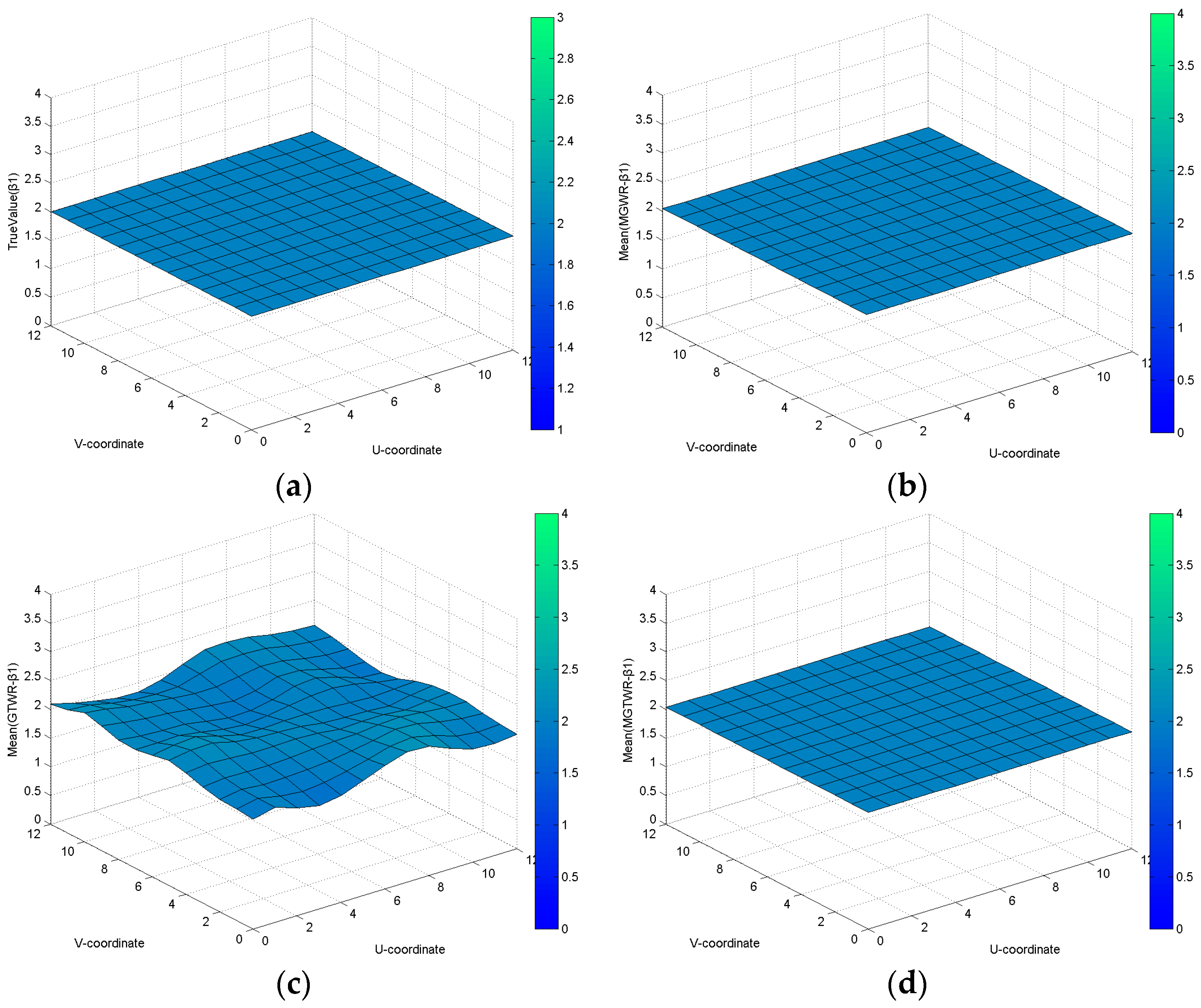
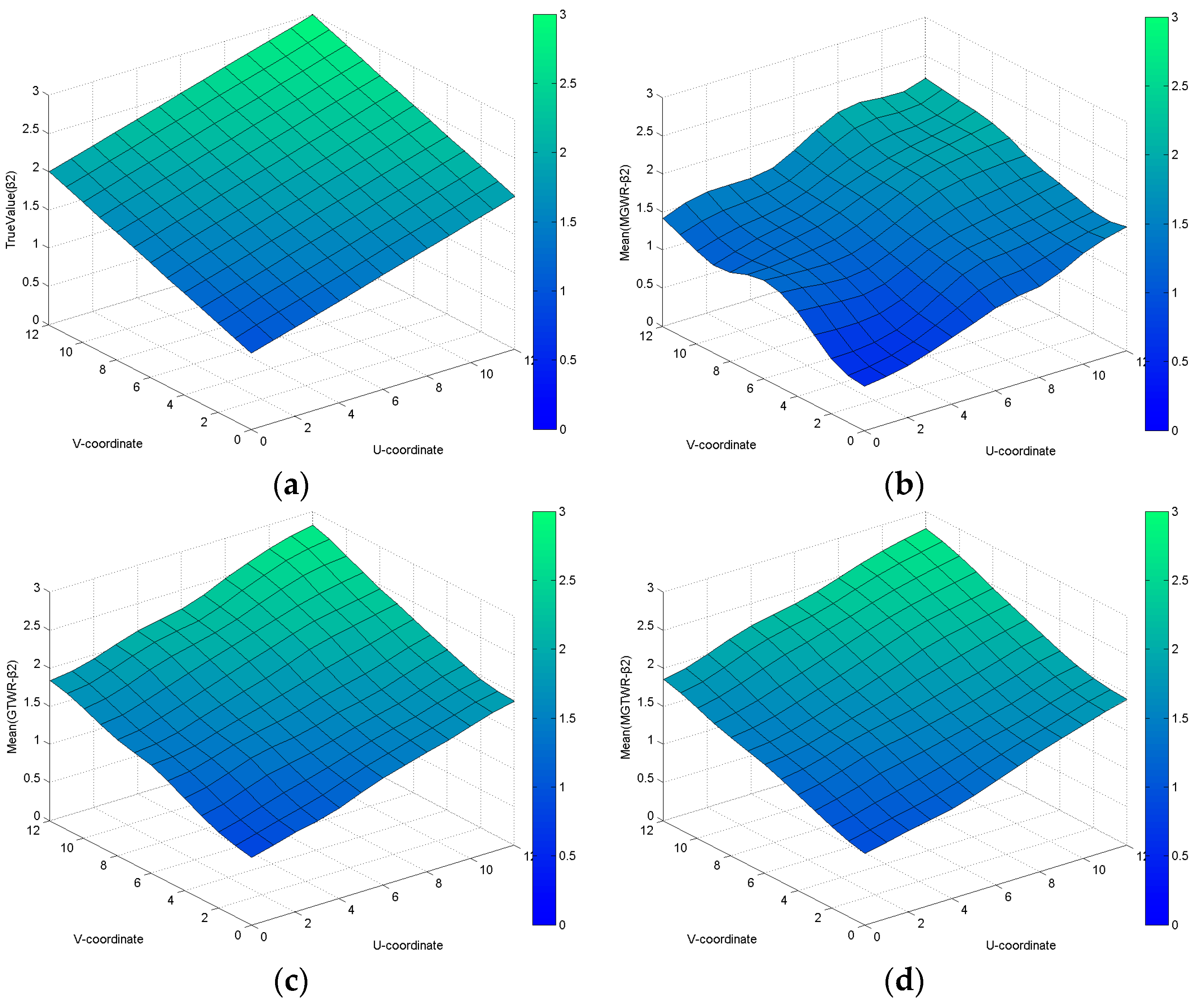
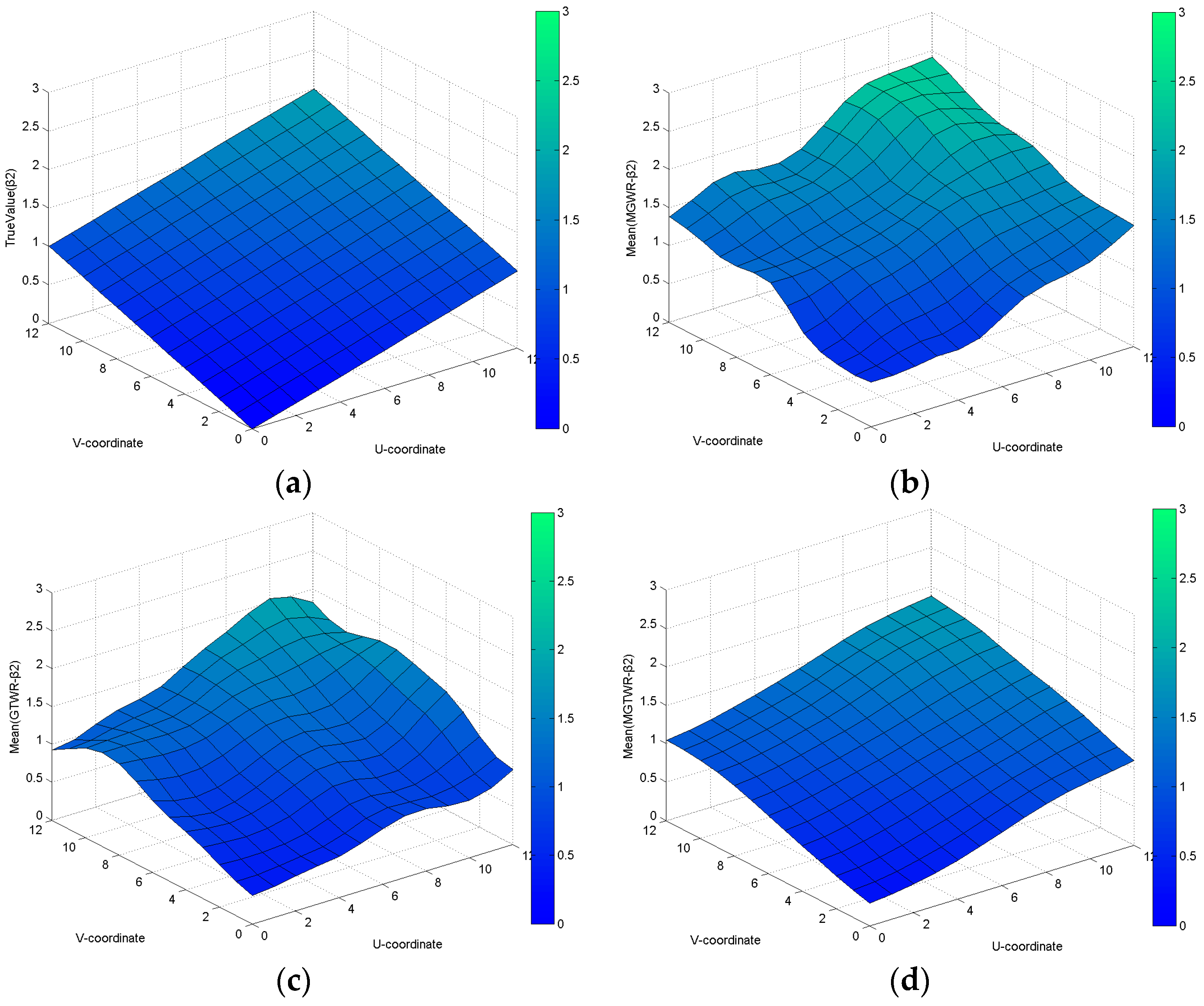
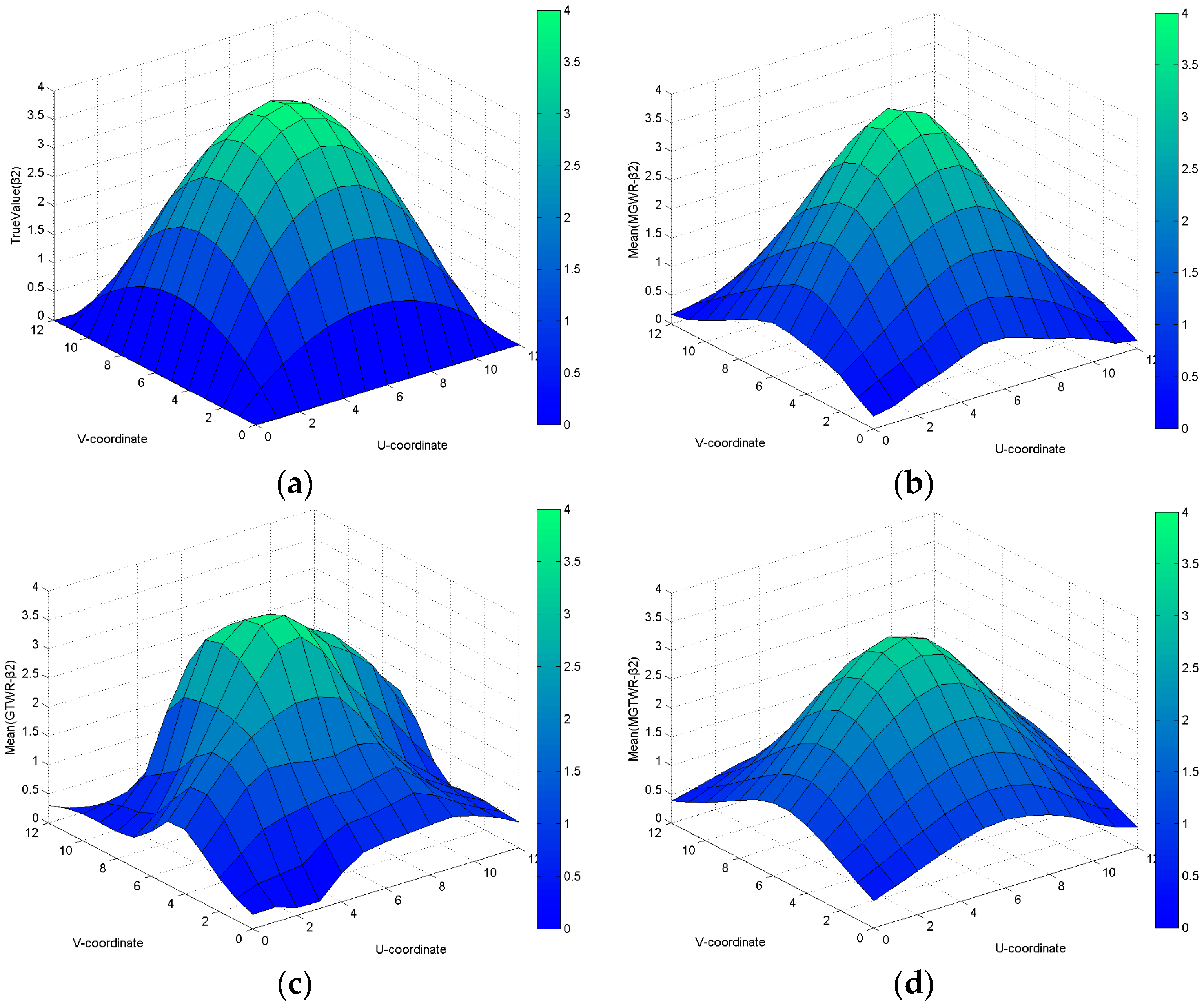
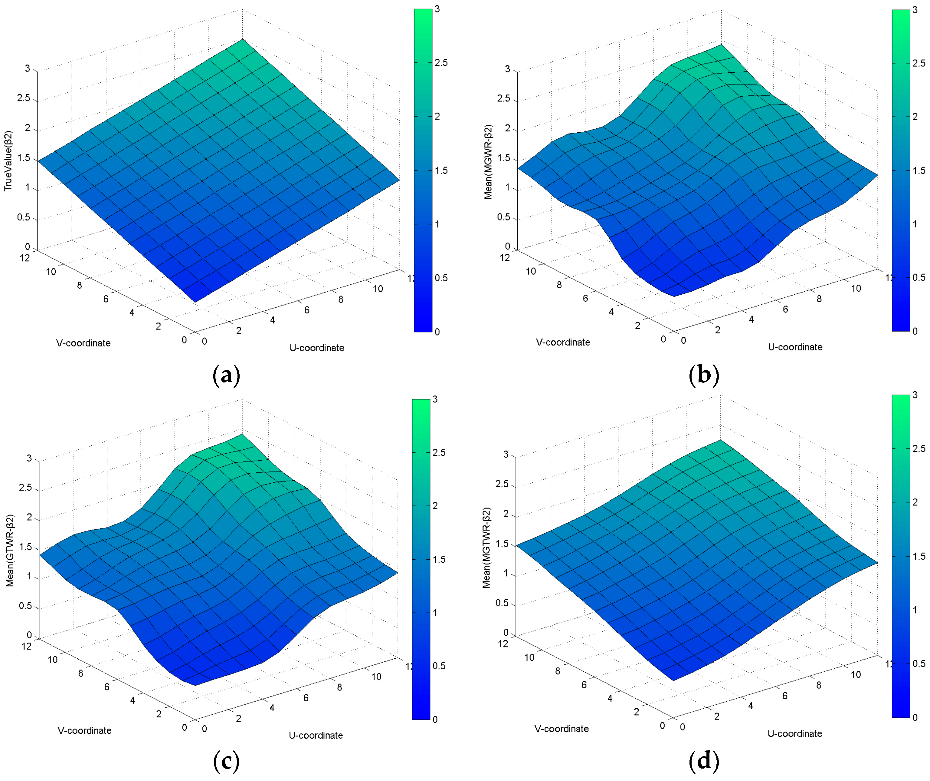
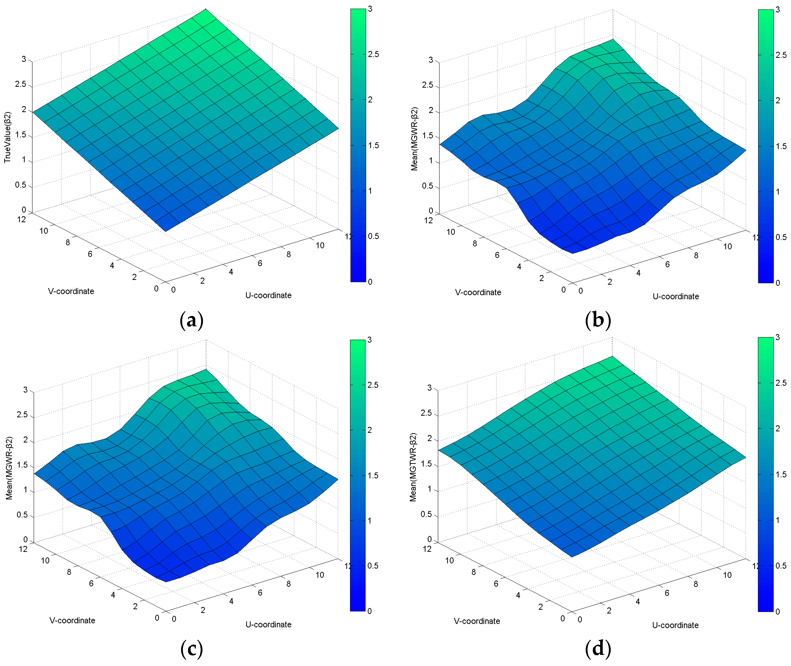
3.1. Simulation Experiments
- Dataset 1: ;
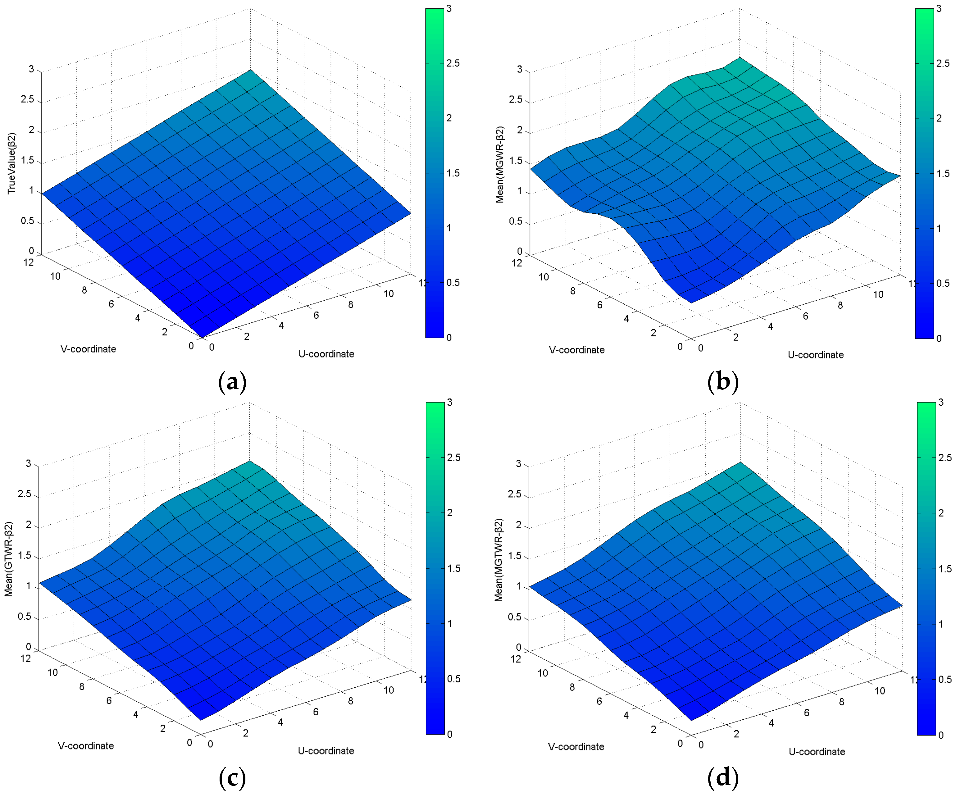
- Dataset 2: and
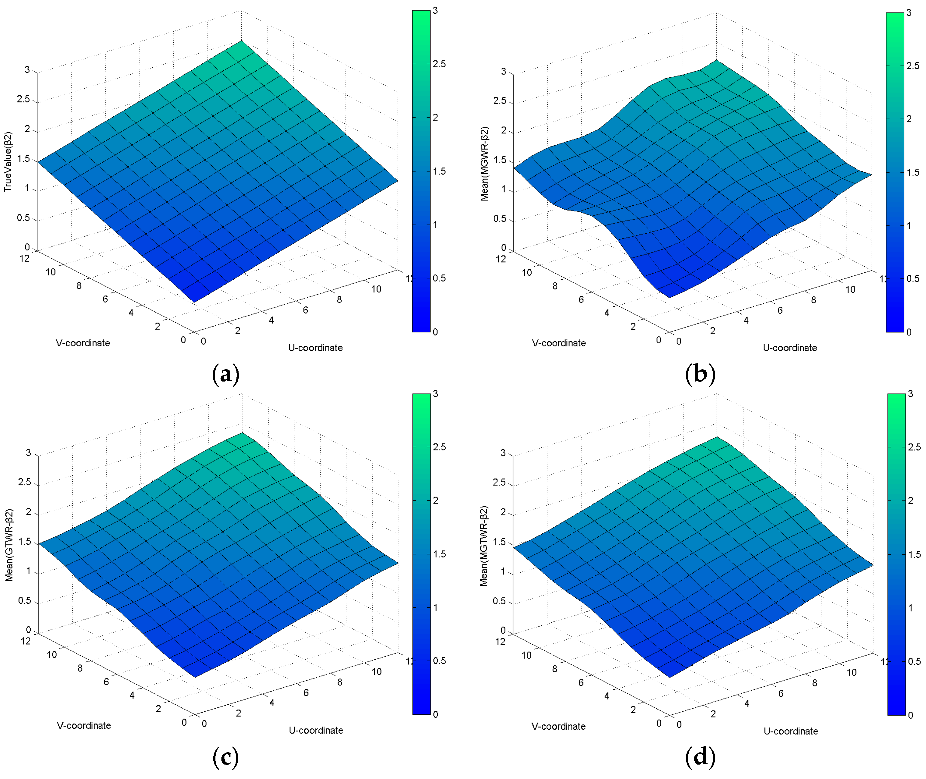
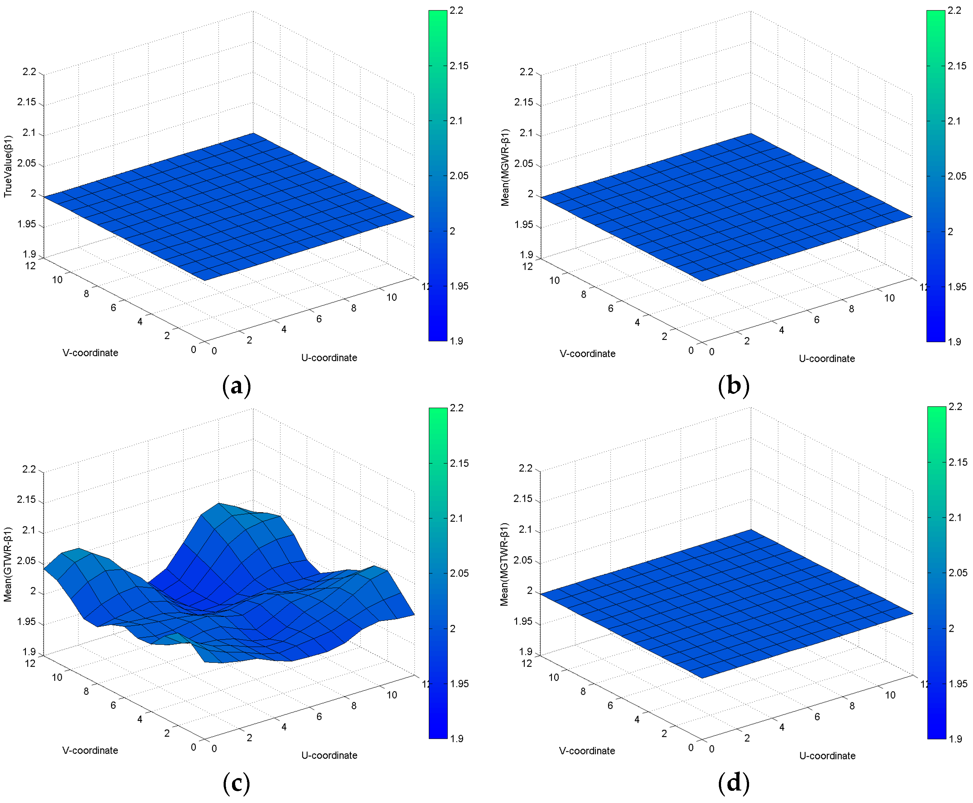
- Dataset 3:
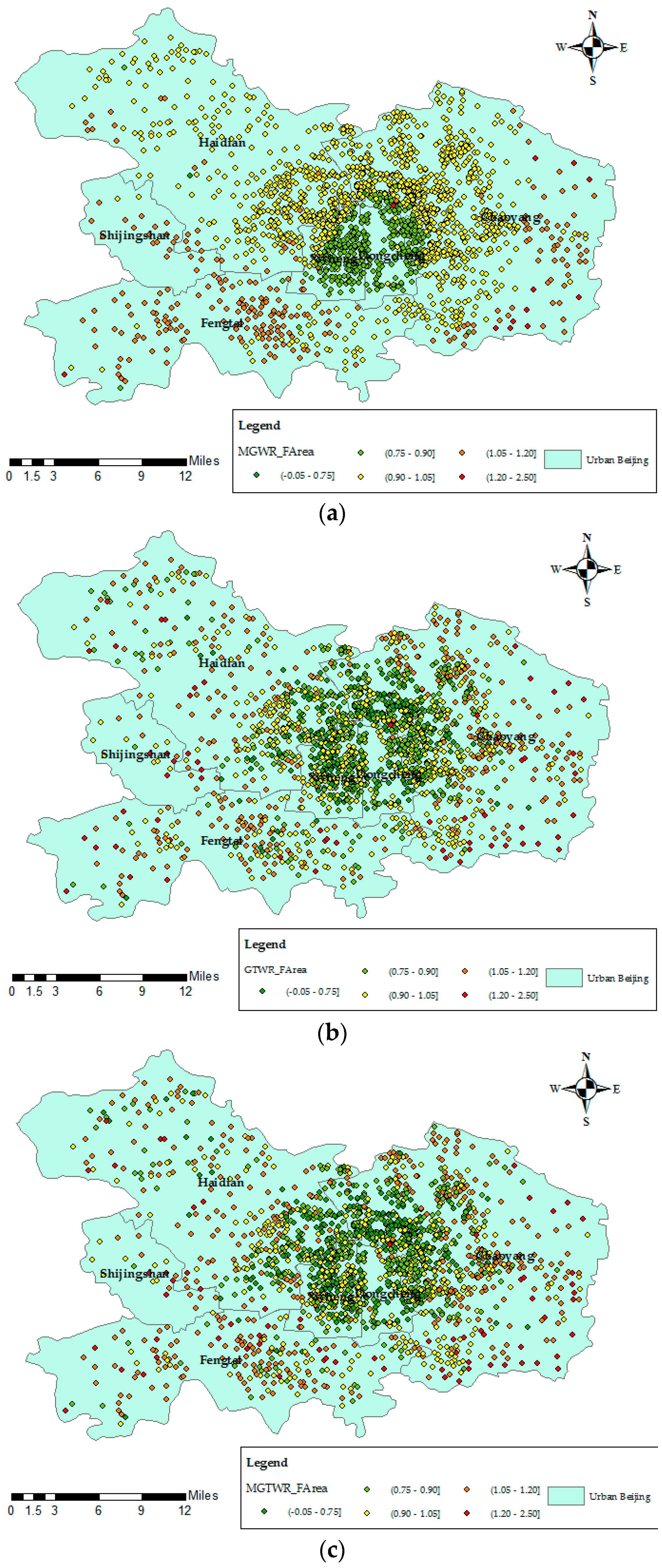
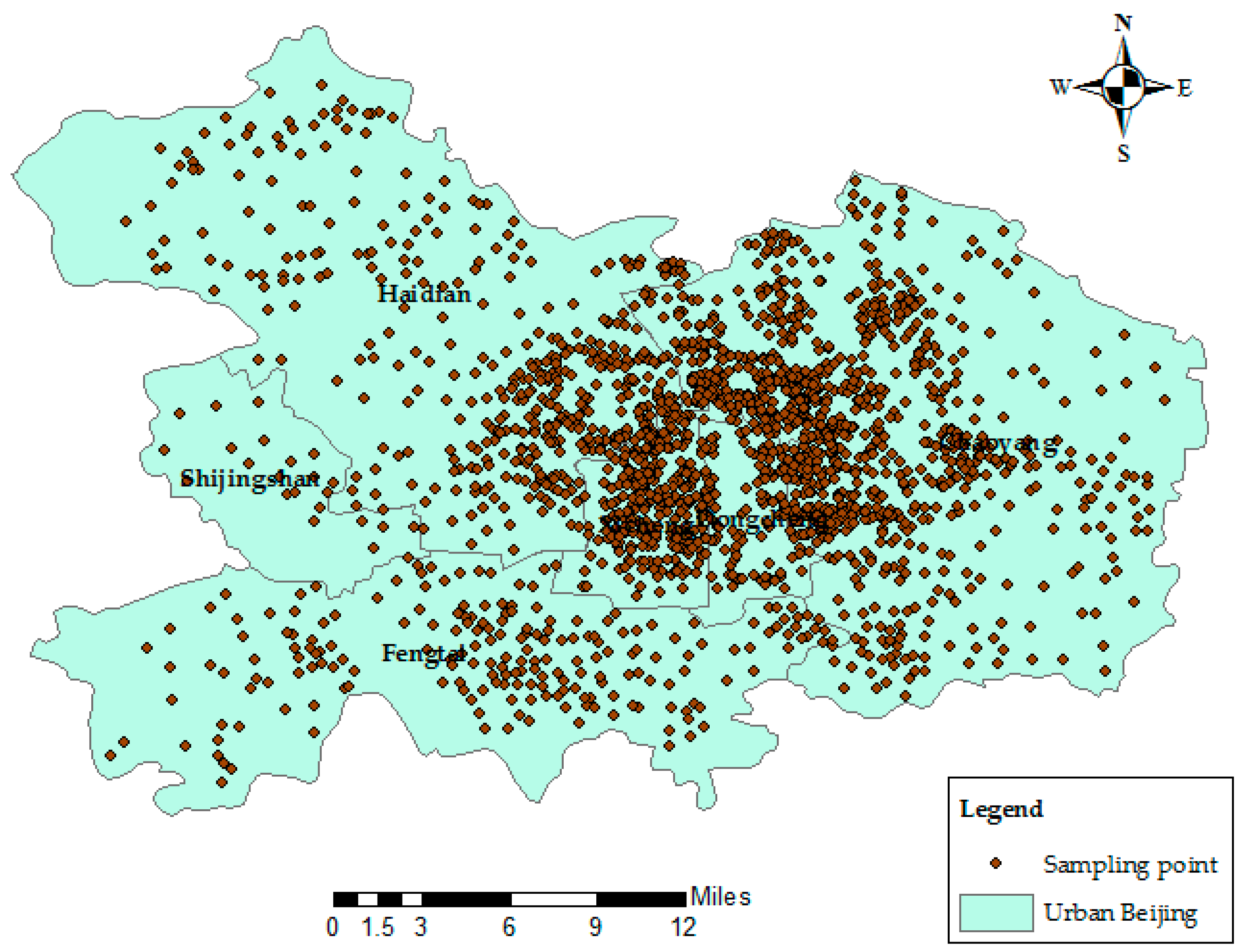
3.2. The Real Data Experiments
3.3. Discussion
- Condition 1: global stationarity and spatial non-stationarity;
- Condition 2: spatial-temporal non-stationarity;
- Condition 3: global stationarity and spatial-temporal non-stationarity.
4. Conclusions
Acknowledgments
Author Contributions
Conflicts of Interest
References
- Brunsdon, C.; Fotheringham, A.S.; Charlton, M.E. Geographically weighted regression: A method for exploring spatial nonstationarity. Geogr. Anal. 1996, 28, 281–298. [Google Scholar] [CrossRef]
- Yin, J.; Gao, Y.; Du, Z.; Wang, S. Exploring multi-scale spatiotemporal twitter user mobility patterns with a visual-analytics approach. ISPRS Int. J. Geo-Inf. 2016, 5. [Google Scholar] [CrossRef]
- Luan, H.; Quick, M.; Law, J. Analyzing local spatio-temporal patterns of police calls-for-service using Bayesian integrated nested laplace approximation. ISPRS Int. J. Geo-Inf. 2016, 5. [Google Scholar] [CrossRef]
- Subasinghe, S.; Estoque, C.R.; Murayama, Y. Spatiotemporal analysis of urban growth using GIS and remote sensing: A case study of the Colombo metropolitan area, Sri Lanka. ISPRS Int. J. Geo-Inf. 2016, 5. [Google Scholar] [CrossRef]
- Brunsdon, C.; Fotheringham, A.S.; Charlton, M. Some notes on parametric significance tests for geographically weighted regression. J. Reg. Sci. 1999, 39, 497–524. [Google Scholar] [CrossRef]
- Fotheringham, A.S.; Brunsdon, C.; Charlton, M. Geographically Weighted Regression; Wiley: Chichester, UK, 2002. [Google Scholar]
- Wang, N.; Mei, C.-L.; Yan, X.-D. Local linear estimation of spatially varying coefficient models: An improvement on the geographically weighted regression technique. Environ. Plan. A 2008, 40, 986–1005. [Google Scholar] [CrossRef]
- Cho, S.; Lambert, D.M.; Kim, S.G.; Jung, S. Extreme coefficients in geographically weighted regression and their effects on mapping. GISci. Remote Sens. 2009, 46, 273–288. [Google Scholar] [CrossRef]
- Song, W.; Jia, H.; Huang, J.; Zhang, Y. A satellite-based geographically weighted regression model for regional PM2.5 estimation over the Pearl River Delta region in China. Remote Sens. Environ. 2014, 154, 1–7. [Google Scholar] [CrossRef]
- You, W.; Zang, Z.; Zhang, L.; Li, Y.; Pan, X.; Wang, W. National-scale estimates of ground-level PM2.5 concentration in China using geographically weighted regression based on 3 km resolution MODIS AOD. Remote Sens. 2016, 8, 184. [Google Scholar] [CrossRef]
- Wheeler, D.; Tiefelsdorf, M. Multicollinearity and correlation among local regression coefficients in geographically weighted regression. J. Geogr. Syst. 2005, 7, 161–187. [Google Scholar] [CrossRef]
- Zhang, H.; Mei, C. Local least absolute deviation estimation of spatially varying coefficient models: Robust geographically weighted regression approaches. Int. J. Geogr. Inf. Sci. 2011, 25, 1467–1489. [Google Scholar] [CrossRef]
- Harris, R.; Dong, G.; Zhang, W. Using contextualized geographically weighted regression to model the spatial heterogeneity of land prices in Beijing, China. Trans. GIS 2013, 17, 901–919. [Google Scholar] [CrossRef]
- Lu, B.; Charlton, M.; Harris, P.; Fotheringham, A.S. Geographically weighted regression with a non-Euclidean distance metric: A case study using hedonic house price data. Int. J. Geogr. Inf. Sci. 2014, 28, 660–681. [Google Scholar] [CrossRef]
- Lu, B.; Charlton, M.; Brunsdon, C.; Harris, P. The Minkowski approach for choosing the distance metric in geographically weighted regression. Int. J. Geogr. Inf. Sci. 2016, 30, 351–368. [Google Scholar] [CrossRef]
- Huang, B.; Wu, B.; Barry, M. Geographically and temporally weighted regression for modeling spatio-temporal variation in house prices. Int. J. Geogr. Inf. Sci. 2010, 24, 383–401. [Google Scholar] [CrossRef]
- Wu, B.; Li, R.; Huang, B. A geographically and temporally weighted autoregressive model with application to housing prices. Int. J. Geogr. Inf. Sci. 2014, 28, 1186–1204. [Google Scholar] [CrossRef]
- Yu, D. Understanding regional development mechanisms in greater Beijing area, China, 1995–2001, from a spatial–temporal perspective. GeoJournal 2014, 79, 195–207. [Google Scholar] [CrossRef]
- Chu, H.-J.; Huang, B.; Lin, C.-Y. Modeling the spatio-temporal heterogeneity in the PM10-PM2.5 relationship. Atmos. Environ. 2015, 102, 176–182. [Google Scholar] [CrossRef]
- Bai, Y.; Wu, L.; Qin, K.; Zhang, Y.; Shen, Y.; Zhou, Y. A geographically and temporally weighted regression model for ground-level PM2.5 estimation from satellite-derived 500 m resolution AOD. Remote Sens. 2016, 8, 262. [Google Scholar] [CrossRef]
- Wrenn, D.H.; Sam, A.G. Geographically and temporally weighted likelihood regression: Exploring the spatiotemporal determinants of land use change. Reg. Sci. Urban Econ. 2014, 44, 60–74. [Google Scholar] [CrossRef]
- Fotheringham, A.S.; Crespo, R.; Yao, J. Geographical and temporal weighted regression (GTWR). Geogr. Anal. 2015, 47, 431–452. [Google Scholar] [CrossRef]
- Mei, C.-L.; He, S.-Y.; Fang, K.-T. A note on the mixed geographically weighted regression model. J. Reg. Sci. 2004, 44, 143–157. [Google Scholar] [CrossRef]
- Wei, C.-H.; Qi, F. On the estimation and testing of mixed geographically weighted regression models. Econ. Model. 2012, 29, 2615–2620. [Google Scholar] [CrossRef]
- Kang, D.; Dall’erba, S. Exploring the spatially varying innovation capacity of the US counties in the framework of Griliches’ knowledge production function: A mixed GWR approach. J. Geogr. Syst. 2016, 18, 125–157. [Google Scholar] [CrossRef]
- Badinger, H.; Egger, P. Fixed effects and random effects estimation of higher-order spatial autoregressive models with spatial autoregressive and heteroscedastic disturbances. Spat. Econ. Anal. 2014, 10, 11–35. [Google Scholar] [CrossRef]
- Akaike, H. Information Theory and an Extension of the Maximum Likelihood Principle. In Proceedings of the second International Symposium on Information Theory, Tsahkadsor, Armenia, 2–8 September 1971; pp. 267–281.
- Hurvich, C.M.; Simonoff, J.S.; Tsai, C.-L. Smoothing parameter selection in nonparametric regression using an improved Akaike information criterion. J. R. Stat. Soc. Ser. B 1998, 60, 271–293. [Google Scholar] [CrossRef]
- Páez, A.; Long, F.; Farber, S. Moving window approaches for hedonic price estimation: An empirical comparison of modelling techniques. Urban Stud. 2008, 45, 1565–1581. [Google Scholar] [CrossRef]
- Peterson, S.; Flanagan, A. Neural Network Hedonic Pricing Models in Mass Real Estate Appraisal. J. Real Estate Res. 2009. Available online: https://papers.ssrn.com/sol3/papers.cfm?abstract_id=1086702 (accessed on 24 January 2017). [Google Scholar]
- Kuşan, H.; Aytekin, O.; Özdemir, İ. The use of fuzzy logic in predicting house selling price. Expert Syst. Appl. 2010, 37, 1808–1813. [Google Scholar] [CrossRef]
- Selim, S. Determinants of house prices in Turkey: A hedonic regression model. Doğuş Üniversitesi Dergisi 2011, 9, 65–76. [Google Scholar]
- Helbich, M.; Brunauer, W.; Vaz, E.; Nijkamp, P. Spatial heterogeneity in hedonic house price models: The case of Austria. Urban Stud. 2013, 51, 390–411. [Google Scholar] [CrossRef]
- Liu, J.; Yang, Y.; Xu, S. A geographically temporal weighted regression approach with travel distance for house price estimation. Entropy 2016, 18, 303. [Google Scholar] [CrossRef]
- Leung, Y.; Mei, C.L.; Zhang, W.X. Statistical tests for spatial nonstationarity based on the geographically weighted regression model. Environ. Plan. A 2000, 32, 9–32. [Google Scholar] [CrossRef]
- Xuan, H.; Li, S.; Amin, M. Statistical inference of geographically and temporally weighted regression model. Pak. J. Stat. 2015, 31, 307–325. [Google Scholar]


| Statistic | MGWR | GTWR | MGTWR | |||
|---|---|---|---|---|---|---|
| Bandwidth | Bandwidth | τ | Bandwidth | τ | ||
| Dataset 1 | Min | 1.34 | 1.41 | 0.01 | 2.075 | 0.01 |
| Mean | 1.655 | 1.844 | 0.01 | 2.4425 | 0.01 | |
| Max | 1.83 | 2.18 | 0.01 | 2.95 | 0.01 | |
| Dataset 2 | Min | 1.69 | 1.48 | 0.129 | 1.725 | 0.2095 |
| Mean | 1.872 | 1.774 | 0.2396 | 2.0575 | 0.409 | |
| Max | 2.04 | 1.9 | 0.366 | 2.25 | 0.6085 | |
| Dataset 3 | Min | 1.69 | 1.9 | 0.287 | 2.25 | 0.6085 |
| Mean | 1.809 | 1.984 | 0.3265 | 2.5125 | 0.78805 | |
| Max | 1.9 | 2.11 | 0.445 | 2.95 | 1.207 | |
| MGWR | GTWR | MGTWR | MGTWR/MGWR Improvement | MGTWR/GTWR Improvement | |
|---|---|---|---|---|---|
| Dataset 1 | 592.1566 | 635.0128 | 589.45 | 2.7066 | 45.5628 |
| Dataset 2 | 7168.606 | 6493.464 | 6532.238 | 36.368 | −38.774 |
| Dataset 3 | 6516.37 | 6439.214 | 6403.558 | 112.812 | 35.656 |
| Abbreviation | Description | Units |
|---|---|---|
| LnPrice | Residential sales price | RMB |
| LnPRatio | Log of the resident plot ratio | — |
| LnGRatio | Log of the resident greening ratio | — |
| LnFArea | Log of the housing area | Square meter |
| LnPFee | Log of the resident property management fee | RMB/Square meter |
| LnDpriSchool | Log of the distance to the nearest primary school | Meter |
| LnDShMall | Log of the distance to the nearest shopping mall | Meter |
| Age | Age of the building (with 1980 as the base year) | Year |
| Intercept | LnPRatio | LnGRatio | LnFArea | LnPFee | LnDpriSchool | LnDShMall | Age | |
|---|---|---|---|---|---|---|---|---|
| Spatial | <0.001 * | >0.1 | <0.001 * | <0.001 * | >0.3 | <0.05 * | >0.1 | <0.05 * |
| Spatial-temporal | <0.001 * | <0.001 * | <0.001 * | <0.001 * | >0.05 | <0.001 * | <0.001 * | <0.001 * |
| Min | Lower Quartile | Mean | Median | Upper Quartile | Max | SD | |
|---|---|---|---|---|---|---|---|
| Intercept | −6.5845 | 1.1898 | 1.6174 | 1.9083 | 2.2080 | 3.1061 | 0.9080 |
| LnPRatio | −0.3655 | −0.0126 | 0.0024 | −0.0043 | 0.0084 | 0.2503 | 0.0294 |
| LnGRatio | −2.0528 | −0.1575 | −0.0177 | −0.0591 | 0.1127 | 2.1998 | 0.2201 |
| LnFArea | −0.0487 | 0.8066 | 0.9286 | 0.942 | 1.0557 | 2.4133 | 0.1731 |
| LnPFee | 0.0223 | 0.0223 | 0.0223 | 0.0223 | 0.0223 | 0.0223 | 0.0000 |
| LnDpriSchool | −0.0667 | −0.0167 | −0.0114 | −0.0104 | −0.0053 | 0.4763 | 0.0165 |
| LnDShMall | −0.0901 | 0.0105 | 0.0241 | 0.0230 | 0.0380 | 0.6799 | 0.0291 |
| MSE | R2 | R2adj | AIC | |
|---|---|---|---|---|
| MGWR | 0.0958 | 0.8135 | 0.8129 | 1113.1958 |
| GTWR | 0.078 | 0.8482 | 0.8477 | 987.7558 |
| MGTWR | 0.0691 | 0.8654 | 0.8649 | 858.9917 |
| MGTWR/MGWR Improvement | 27.87% | 6.38% | 6.40% | 254.20 |
| MGTWR/GTWR Improvement | 11.41% | 2.03% | 2.03% | 128.76 |
© 2017 by the authors. Licensee MDPI, Basel, Switzerland. This article is an open access article distributed under the terms and conditions of the Creative Commons Attribution (CC BY) license ( http://creativecommons.org/licenses/by/4.0/).
Share and Cite
Liu, J.; Zhao, Y.; Yang, Y.; Xu, S.; Zhang, F.; Zhang, X.; Shi, L.; Qiu, A. A Mixed Geographically and Temporally Weighted Regression: Exploring Spatial-Temporal Variations from Global and Local Perspectives. Entropy 2017, 19, 53. https://doi.org/10.3390/e19020053
Liu J, Zhao Y, Yang Y, Xu S, Zhang F, Zhang X, Shi L, Qiu A. A Mixed Geographically and Temporally Weighted Regression: Exploring Spatial-Temporal Variations from Global and Local Perspectives. Entropy. 2017; 19(2):53. https://doi.org/10.3390/e19020053
Chicago/Turabian StyleLiu, Jiping, Yangyang Zhao, Yi Yang, Shenghua Xu, Fuhao Zhang, Xiaolu Zhang, Lihong Shi, and Agen Qiu. 2017. "A Mixed Geographically and Temporally Weighted Regression: Exploring Spatial-Temporal Variations from Global and Local Perspectives" Entropy 19, no. 2: 53. https://doi.org/10.3390/e19020053
APA StyleLiu, J., Zhao, Y., Yang, Y., Xu, S., Zhang, F., Zhang, X., Shi, L., & Qiu, A. (2017). A Mixed Geographically and Temporally Weighted Regression: Exploring Spatial-Temporal Variations from Global and Local Perspectives. Entropy, 19(2), 53. https://doi.org/10.3390/e19020053