1. Introduction
This paper is part of a series on the problem of how to measure statistical evidence on a properly calibrated scale. In earlier work we proposed embedding the measurement problem in a novel information dynamic theory [
1,
2]. Vieland [
3] proposed that this theory is grounded in two laws: (1) a form of the likelihood principle, viewed as a conservation principle on a par with the 1st law of thermodynamics; and (2) a law involving information loss incurred by the data analytic process itself through data compression, which she related to (at least one form of) the 2nd law of thermodynamics.
By data compression we mean what Landauer [
4] called a
logically irreversible operation on a set of (statistical) data. For example, condensing a list of measurements
, into the summary statistic
represents a loss of information regarding the individual
values. In order to perform inferences regarding the mean, this compression is necessary. However, once done it cannot be undone, in that the original list of measurements cannot be reconstructed from
alone. In this sense the operation of compression is logically irreversible, and it incurs a reduction in entropy, that is, in what we might call the “system” entropy, or the entropy associated with the compressed data.
Here we consider not only the entropy remaining after data compression, but also the entropy lost, or dissipated, in the process of compression. Illustrating throughout with the binomial distribution, we show a wholly information-based connection to Landauer’s principle, and we comment on the potential importance of keeping track of this lost information as part of the data analytic process.
2. Information Decomposition under Data Compression
Following [
3], we begin by considering independent Bernoulli trials, each of which produces either a success (
S) or a failure (
F). One trial produces 1 bit (=
) of sequence information, in that after recording the outcome we know which of two possible things actually happened. For
n trials, define the total sequence information as
If one knows the exact sequence y of observations, e.g., , then one knows which choice or event occurred at each of the n trials, and thus one possesses the full sequence information represented in (1).
In contrast, if only the total number of successes (
x) is known or recorded, the information about the sequence of successes and failures is lost and cannot be recovered or reconstructed from
x alone. (Here and throughout the paper we assume that
n is also known). The data have been compressed from a full description to the summary measure
x. We refer to this as “binomial compression”. The combinatoric coefficient
gives the number of sequences compatible with the observed
x, and thus indexes the information
loss, since one no longer knows which of those sequences actually gave rise to the observed value of
x. Define the lost information as
The difference between (1) and (2) gives the “remaining” or “compressed” information,
so that
(Vieland [
3] referred to (3) as
, viewed as the change in sequence information, following the notation of Duncan and Semura [
5,
6]).
The compressed information (3) can be viewed in terms of the ratio of which is the log, that is, the ratio . When only x is known, it is as if the total information represented in (1) has been “spread out” or averaged among the possible sequences compatible with the observed x.
Intermediate setups exist that fall between the two extremes of preserving all sequence information vs. discarding all of it. For example, one can perform some of the trials, and record the number of successes (but not their sequence) within that set or “batch” of trials, then perform the rest of the trials and record the number of successes in the second batch. (e.g., there could be a first batch of 3 trials, with 2 successes, followed by a second batch of 2 trials, with 1 success). The data are compressed, but less so than in the preceding section. In these cases, equals the sum of the individual log combinatoric coefficients for each batch—a sum that cannot exceed in (2).
Note that here we are concerned with information defined in terms of the number of possible sequences of observations. Below we will generalize this concept to Shannon information and its expected value, Shannon entropy. A very different kind of information—Fisher information [
7]—plays a role in much statistical theory. While we comment briefly on one difference between Shannon information and Fisher information below, our focus here remains on information in the “number of sequences” or Shannon sense.
3. Entropy Decomposition under Data Compression
We now turn from information to Shannon entropy. As is well known, Shannon’s basic unit of information is the negative log of the probability, and Shannon entropy is the expected value of this information. For a single Bernoulli trial, the Shannon entropy [
8] becomes
, i.e., the negative expected value of
from a single trial with outcome sequence
y (
p = probability of
S in a single trial,
q = 1 –
p). When we know the full sequence information, the Shannon entropy for
n Bernouilli trials is
. Each value of
i represents one of the
possible sequences
y, and each sequence has probability
, with
x equaling the number of successes in that sequence. Combining all sequences
y with the same value of
x yields (5), which is the entropy for a single trial multiplied by
n,
Shannon [
8] (p. 10) showed that the joint entropy for two variables
x and
y can be decomposed as
To apply this to the binomial distribution, define
as the probability of count
x, and
as the probability of sequence
y, given count
x. (For example, with
,
, and
). Then Shannon’s
becomes
Here we are following the notation of Attard [
9], who decomposes the Shannon entropy using
x for the macrostates of a physical system and
y for the microstates, so that the “complete” (joint) entropy of the macro-
and microstates,
, can be expressed as the entropy of the macrostates,
, plus the conditional entropy of the microstates given the macrostates,
(see also Toffoli [
10]).
This much is familiar. What has not been noted before, to our knowledge, is how this entropy decomposition relates to the sequence information decomposition from
Section 2 above. When only the number of successes
x (and
n) is recorded, the Shannon entropy is
That is, the entropy in this situation is the quantity in Equation (5), reduced by the expected value of .
We can recognize
as corresponding to
in (2) (here
functions as a random variable), and its (negative) expected value equals
in Shannon’s decomposition:
Thus, the conditional entropy of y (the sequences, or microstates) given (i.e., consistent with) a specified count (or macrostate) x, is a straightforward generalization of in (2).
Moreover, writing (5) as
, (7) as
, and (8) as
yields
Thus, Shannon’s decomposition (6) aligns with the “total”, “comp,” and “lost” breakdown in (9), and also recapitulates the decomposition of the sequence information in (4).
Compressing the data into “batches” also functions analogously to what was seen in
Section 2: The entropy for
batches of size
equals the sum of the entropies of the individual batches
.
One can also decompose the information itself, rather than the expected information: The probabilities corresponding to the entropies in (6) or (9) are . The joint probability (as well as its log, the joint Shannon information) cleaves neatly into the “count” component, , which is a function of p, and the “sequence conditioned on count” component, , which is not a function of p.
Indeed, for the binomial distribution, the likelihood function
, for
k an arbitrary constant, is proportional to the full probability, including sequence information, despite the fact that it represents the compressed data. That is, losing the
sequence information does not entail any loss of information
about p; for given
n, all the information about
p is conveyed by
x. Thus binomial data compression, which affects the Shannon information, does not affect the Fisher information, highlighting the existence of (at least) two distinct concepts of information here. Equivalently,
L(
p) is a sufficient statistic for
p [
7,
11], so that relative quantities such as the likelihood ratio (LR) and the Kullback–Leibler divergence (KLD) [
12] are also unaffected by binomial compression. E.g., the LR comparing
and
is
, with the combinatoric term
canceled out. Thus “batching” also has no impact on the LR or the KLD, despite the close connection between the latter quantity and Shannon entropy itself.
Of course there are other ways of compressing Bernoulli data that do affect information about
p, e.g., combining genotypes into phenotypes [
13], or defining a random variable that represents the number of transitions
and
occurring in
n trials. In such situations there is genuine loss of information
about p inherent in the compression of the data; the likelihood, the LR, KLD and Fisher information are all affected as well.
4. Data Compression and Information Loss
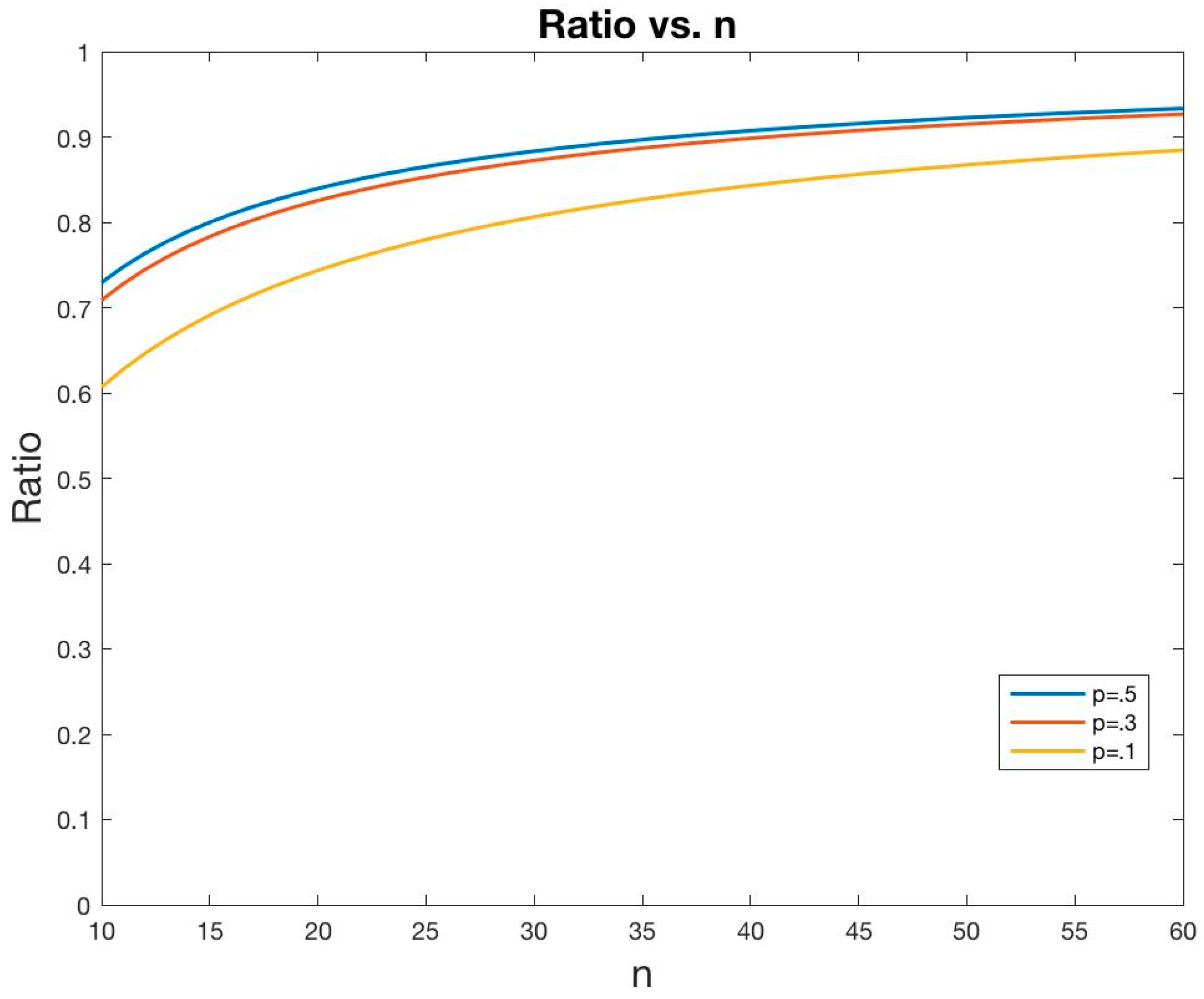
Figure 1 shows that the ratio
increases with
n, asymptotically approaching 1. The amount of “lost” entropy increases faster than does the total entropy. This is related to Landauer’s [
4] principle: logically irreversible data compression
reduces the entropy of the “system” (i.e.,
), but it also creates what physicists would call non-information-bearing degrees of freedom, or entropy dissipated into the “environment” (i.e.,
), such that there is a net increase in total entropy. Moreover, while the system entropy
increases with
n, the proportion
dissipated into the environment increases faster. We could express this by saying that the efficiency with which new data change
decreases as
increases. Here we have made no reference to physical manifestations of information or its erasure through data compression, but
Figure 1 suggests that we might need to take account of not only the remaining information, but also the lost information, when we consider the complete “dynamics” of informational systems.
Vieland [
3] proposed, following the lead of Duncan and Semura [
5], that evidence
E plays a parallel role to absolute temperature T in “linking” the bookkeeping required to track two different types of information, through the relationship
, where
k is a constant (not necessarily equal to Boltzmann’s constant),
is the total (evidential) information transferred in with new data, and
is the net loss of (combinatoric) information incurred by data compression. (In
Section 2 above we referred to
as
; we then extended this to the dissipated entropy
in
Section 3).
One distinctive property of
E as defined by this equation is that, as a function of increasing
n, it increases in a concave-down manner [
2,
14]: All other things being equal,
E increases more slowly, the stronger it is. This seems to accord with what we mean when we talk about statistical evidence. For example, adding 10 heads to a data set with (
n = 2, X = 2) increases the evidence that the coin is biased far more than does adding those same 10 heads to a data set with (
n = 200, X = 200), since in the latter case the evidence in favor of bias is already overwhelming. To our knowledge,
E is unique among statistical evidence measures in conforming to this behavior of the evidence itself. By contrast, the LR, the Bayes ratio and the
p-value all show exponential change with increasing
n in such situations. Thus in at least this one regard,
E appears to offer distinct advantages over other approaches to statistical evidence, insofar as its behavior better conforms to what we mean when we speak about evidence. This concave-down feature appears to be related to the basic relationship shown in
Figure 1, whereby the lost, or dissipated, entropy increases more quickly than the total entropy, as a function of increasing
n.
5. Discussion
In this paper we have pursued the idea of information lost through data compression, as occurs in the course of any data analysis. Following [
3] we considered a decomposition of the entropy into
,
, and
, or the total, lost and compressed (remaining) components, respectively. Using the binomial distribution, we illustrated the fact that, as Jaynes [
15] instructed us, the effects of data compression on these entropy components depends on what we know about the data generation process—e.g., whether the full sequence of results or only the total number of successes
x is recorded, or whether we have partial knowledge of which outcomes occurred in each of several sub-experiments.
We also considered the relationship between our entropy decomposition and two others: Landauer’s [
4] decomposition of physical entropy change for logically irreversible data erasure operations into information-bearing degrees of freedom (the system entropy) and remaining degrees of freedom (the medium entropy, which absorbs heat dissipated during the process); and Shannon’s [
8] decomposition of the Shannon entropy for two variables into a marginal and a conditional component (per our Equation (6); see also Attard [
9], who gave a corresponding decomposition in terms of the joint and marginal entropies for macrostates and microstates of a statistical mechanical system). What we have shown here is that there is an interpretive connection between these three decompositions. From a mathematical point of view, they have the same form.
Viewing matters through the lens of the information loss inherent in data compression let us show in addition that the ratio increases with n, that is, the amount of “lost” entropy increases faster than does the total entropy. This can be described as a decrease in the efficiency with which new data convey information, as the total amount of information increases. We noted that this accords with intuition, in the sense that we learn less from a fixed increment of new data, the more we already know.
As mentioned above, Vieland [
3] was interested in data compression in the context of deriving a new measure of statistical evidence. We noted that the information dynamic evidence measure
E [
2] is unique among alternative evidence measures (including the
p-value, likelihood ratio and Bayes factor) in increasing more slowly (being “concave-down”), all other things being equal, with increasing
n. Ordinarily, statistical analyses focus only on what we have called
itself (extending the definition to cover distributions other than the binomial). That is, statistical analyses commence
after the data have been suitably compressed into, say, the count
x of “successes” on
n trials, or the mean
of a set of numbers, etc. No account is taken of the information lost in this process. This same point applies to most statistical treatments of entropy (e.g., Kullback [
16], Soofi [
17], Osteyee and Good [
18] and many others), as well as other approaches to measurement of statistical evidence with which we are familiar (e.g., Edwards [
19]; Royall [
20]; Taper and Lele [
21]; Bickel [
22]; Stern and Pereira [
23]; Evans [
24]; Zhang [
25]; among others).
While details remain to be worked out, we believe that E’s unique “concave-down” behavior is related to our use of a complete accounting of all components of the entropy decomposition in our underlying information dynamic framework. We are unaware of any other statistical context in which tracking “lost” information, or a form of information that is dissipated during the data analytic process, plays a central role. However, given the relationships among the various forms of entropy decomposition considered in this paper, we propose as a novel postulate that keeping the books for this information lost through data compression may be essential to a complete understanding of data analysis as an information-transformation process.


