Abstract
It is a relatively well-known fact that in problems of Bayesian model selection, improper priors should, in general, be avoided. In this paper we will derive and discuss a collection of four proper uniform priors which lie on an ascending scale of informativeness. It will turn out that these priors lead us to evidences that are closely associated with the implied evidence of the Bayesian Information Criterion (BIC) and the Akaike Information Criterion (AIC). All the discussed evidences are then used in two small Monte Carlo studies, wherein for different sample sizes and noise levels the evidences are used to select between competing C-spline regression models. Also, there is given, for illustrative purposes, an outline on how to construct simple trivariate C-spline regression models. In regards to the length of this paper, only one half of this paper consists of theory and derivations, the other half consists of graphs and outputs of the two Monte Carlo studies.
1. Introduction
Using informational consistency requirements, Jaynes [1] derived the form of maximal non-informative priors for location parameters, that is, regression coefficients, to be uniform. However, this does not tell us what the limits of these uniform probability distributions should be, that is, what particular uniform distribution to use. If we are faced with a parameter estimation problem, then these limits of the uniform prior are irrelevant, as we may scale the product of the improper uniform prior and the likelihood to one, which gives us a properly normalized posterior for our regression coefficients. However, if we are faced with a problem of model selection, then the volume covered by the uniform prior is an integral part of the evidence which is used to rank the various competing regression models.
In this paper we will give the four proper uniform priors originally derived in [2]. These priors lie on an ascending scale of informativeness. It will turn out, as we discuss the Bayesian Information Criterion (BIC), the Akaike Information Criterion (AIC), and the results of a small Monte Carlo study, that these priors lead us to evidences that are closely associated with the implied evidences of the BIC and the AIC, as these evidences fill in the space between and around the BIC and AIC on a continuum of conservativeness, in terms of the number of parameters of the chosen regression analysis models.
This paper is structured as follows. First we give an introduction to the evidence construct, that “too-often-ignored half of Bayesian inference” [3], as we give an outline on how to use these evidences in Bayesian model selection. Then we describe the normal multiple regression models for both known and unknown s, after which we specify the conditions under which improper priors become problematic for model selection. This specification brings us naturally to a continuum of informativeness on which priors of regression coefficients may be located. After these preliminaries, we proceed to give the derivations of the four proper uniform priors, originally derived in [2], by way of the results in [4], which are neither grossly ignorant nor grossly knowledgeable. Having checked the coverage of these priors, we address the question what constitutes data and what constitutes prior information. We then discuss the evidences that are associated with our proper priors, as we connect these evidences to the BIC and AIC reference procedures and give the posterior probability distribution of the unknown regression coefficients and the consequent predictive probability distribution that is associated with these proper priors. In Appendix A we report on two small Monte Carlo studies with the C-spline regression models, in order to give the reader a sense for all the discussed evidences. Also, a collection of three simple trivariate C-spline regression models will be discussed in Appendix B, in order to provide the reader with a low-level, hands-on introduction into C-splines [5].
2. The Evidence and Bayesian Model Selection
Bayesian probability theory has four fundamental constructs, namely, the prior, the likelihood, the posterior, and the evidence. These constructs are related in the following way:
Most of us will be familiar with the prior, likelihood, and posterior. However, the evidence concept is less universally known, as most people come to Bayes by way of the more compact relationship [6]:
which does not make any explicit mention of the evidence construct. In what follows, we will employ the correct, though notationally more cumbersome, relation (1), and forgo of the more compact, but incomplete, Bayesian shorthand (2). This is done so the reader may develop some feeling for the evidence construct, and how this construct relates to the other three Bayesian constructs (i.e., the prior, likelihood, and posterior.)
Let be the prior of some parameter , where I is the prior information model of the unknown . Let be the probability of the data D conditional on the value of parameter and the likelihood model M which is used; the probability of the data is also known as the likelihood of the parameter . Let be the posterior distribution of the parameter , conditional on the data D, the likelihood model M, and the prior information model I. Then
where
is the evidence, that is, the marginalized likelihood of both the likelihood model M and the prior information model I.
Now, if we have a set of likelihood models (e.g., a collection of regression models) we wish to choose from, and just the one prior information model I (e.g., an ignorance model), then we may do so by computing the evidence values .
Let and be, respectively, the prior and posterior probability of the likelihood model . Then the posterior probability distribution of these likelihood models is given as
For for , the posterior probabilities (5) will reduce to the normalized evidence values:
So, if we assign equal prior probabilities to our likelihood models , then we may rank these models by way of their respective evidence values, where the model with the highest evidence value is the model which has the highest posterior probability of all the models that were taken into consideration [7,8].
3. The Normal Multiple Regression Model (Known Sigma)
Let the model M for the response vector be
where X is some predictor matrix, is the vector with regression coefficients and is the error vector to which we assign a multivariate normal distribution, that is,
or, equivalently, , where is the identity matrix and is some known standard deviation. By way of a simple Jacobian transformation from to in (8), we then may obtain the likelihood function of the s:
If we assign a uniform prior to the unknown regression coefficients [6]
where C is a yet unspecified normalizing constant, I is the prior information regarding the unknown s which we have at our disposal, and is the prior domain of the s, then the probability distribution of both and is derived as
By integrating the unknown s out of (11) over the prior domain , we obtain the evidence of model M:
The evidence (12) is used both to normalize (11) into a posterior distribution, (1), as well as to choose between competing regression models, (5) and (6). In order to evaluate the evidence (12), we rewrite (11) as [6]
where
We then factor (13) as
The last term in (15) is in the multivariate normal form [6], so it should evaluate to 1 when integrated over the s. Stated differently, for a prior domain which is centered correctly and ‘wide enough’, we have, by way of the factorization (15), that the evidence (12) tends to the equality
By way of (13), (16) and the product rule (1), we obtain the posterior of the unknown s, [6]:
This posterior of the unknown s has a mean of , (14), and a covariance matrix of .
In the parameter estimation problem, that is, the derivation of the posterior distribution (17), any reference to the normalizing constant C of the uniform prior (10) has fallen away. In contrast, in the model selection problem, that is, the derivation of the evidence (16), C is still present.
In closing, note that different predictor matrices correspond with different likelihood models in (5) and (6). It is to be understood that in what follows we will construct proper uniform priors for a generic likelihood model M which has a generic predictor matrix X, as we drop the sub-index j in both X and M in order to remove some of the notational clutter in our equations.
4. The Normal Multiple Regression Model (Unknown Sigma)
In case of unknown , we may assign the Jeffreys prior for scaling parameters [6]:
where A is some normalizing constant, to the unknown in (11), in order to lose this unknown nuisance parameter by way of integration:
where (11) and (18),
We may conveniently factorize (20) as,
The last term in (21) evaluates to 1 when integrated over , as it has the form of an inverted gamma distribution [6], from which it follows that
By integrating the unknown s out of (22) over the prior domain , we obtain the evidence of model M:
In order to evaluate the evidence (23), we rewrite (22) as [6]
We then factor (24) as
where
and where the last term in (25) is in the multivariate Student-t form [6]. So, for a prior domain which is centered correctly and “wide enough”, we have, by way of the factorization (25), that the evidence (23) tends to the equality
If we divide (24) by the evidence (27), we obtain, by way of the product rule (1), the posterior of the unknown s, [6]:
where
This posterior of the unknown s has a mean of , (14), and a covariance matrix of , (29).
Again, in the parameter estimation problem, that is, the derivation of the posterior distribution (28), any reference to the normalizing constant C of the uniform prior (10) has, seemingly, fallen away. In contrast, in the model selection problem, that is, the derivation of the evidence (27), C is still present.
5. The Problem with Improper Priors
In problems of model comparison between competing (regression) models one generally must take care not to use improper priors, be they uniform or not. Since improper priors may introduce inverse infinities in the evidence factors which do not cancel out if one proceeds to compute the posterior probabilities of the respective models [9]. We will demonstrate this fact and its consequences with a simple example in which we assign improper uniform priors to the respective regression coefficients.
Suppose that we want to compare two regression models:
where is an predictor matrix and an , with , and where both and are multivariate normally distributed , where is the identity matrix and is some known standard deviation, (8). Let the uniform prior of a regression coefficient be given as
for . If , then (31) will tend to the improper Jeffreys prior for location parameters [6]:
where “∝” is the proportionality sign that absorbs the normalizing constant . Let the uniform prior of m regression coefficients be given as, (31),
where is an m-dimensional cube which is centered at the origin. Substituting (33) into (10), we find the evidences:
for , where (27)
and is the number of columns in the predictor matrix , and is the regression model estimate (14)
If we assign equal prior probabilities to and , then we find posterior model probabilities, (6) and (34):
as , (30). So, if in (31) we let , then the posterior model probabilities (37) will tend to
It can be seen that the assigning of an improper Jeffreys’ prior to location parameters (32) will make that the regression model with the least number of regression coefficients, or, equivalently, number of predictors, is automatically chosen over any model which has more regression coefficients.
Improper priors can introduce inverse infinities in the evidence factors, as in (37), which do not cancel out if one proceeds to compute the posterior probabilities of the respective models. However, if the parameter in question is shared by all the competing models, like, for example, the parameter in (1), then the inverse infinities will cancel out, like A cancels out in (37). This is why care must be taken to let the prior for the regression coefficients , (10), be proper, while, at the same time, as both a mathematical and a modeling convenience, one may let the prior of , (18), be improper.
6. A Continuum of Informativeness
The Jeffreys prior for location parameters (32),
represents a limit of gross ignorance as we are even ignorant about the possible limits of the parameters . This gross ignorance leads to evidences that are extremely conservative in that they will always choose the regression model with least number of regression coefficients, (38).
An opposite limit of gross knowledgeableness is the empirical “sure thing” prior [3]:
where is the multivariate Dirac delta function for which we have
The evidence that corresponds with the “sure thing” prior may be derived as, (9), (14), (18), (26), (39), and (40):
where the “∝” symbol is used to absorb the factor .
Since an increase in the number of predictors m tends to decrease the length of the error vector , with a limit length of zero as the number of predictors m tends to the sample size N:
we have that, (41) and (42),
So, the gross knowledgeableness of the “sure thing” prior leads to evidences that are extremely liberal in that they will tend to choose regression models which have the largest number of regression coefficients.
In what follows we will derive a suite of priors on the continuum of informativeness that are more informed than the improper Jeffreys prior for location parameters (32) and less knowledgeable than the “sure thing” prior (39). It will be shown that the corresponding evidences, as a consequence, will be less conservative than the evidence (34) in its limit of , and less liberal than the maximum likelihood evidence (41).
7. A Proper Ignorance Prior
We now proceed to construct a more informed, proper (i.e., non-zero) inverse normalizing “constant” C for the prior (10). By way of (7) and (14), we have for a predictor matrix X of rank m that
where
and , (8). Closer inspection of (44) shows us that the parameter space of is constrained by the difference vector .
For the special case where the predictor matrix X is an vector we have that
where is the angle between the predictor vector and the difference vector . Given that , we may by way of (46) put definite bounds on :
So, if we assign a uniform distribution to the regression coefficient , then this uniform distribution is defined on a line-piece of length . It follows that for the case of just the one regression coefficient, the prior (10) is
where (48) is understood to be defined on the interval (47) which is centered at the origin.
In order to generalize (48) to the general multivariate case, we first must generalize (47) to its multivariate case. This may be done as follows [4]. Let X be a predictor matrix consisting of m independent vectors . The vectors , because of their independence, then will span a m-dimensional subspace . It follows, trivially, that we may decompose into a part that lies inside of this subspace and a part that lies outside, say,
where is the part of that is projected on and is the part of that is orthogonal to . The orthogonality of to implies that
for , whereas the fact that is a projection on implies that
where, by construction, (49), (50), and the assumed independence of the ,
Now, because of the independence of the we have that
for . So, if we take the norm of (51) we find
It follows from (54) that the angles in (52) must obey the constraint
Combining (52) and (55), we see that the regression coefficients must lie on the surface of an m-variate ellipsoid centered at the origin and with axes which have respective lengths of
Since
the axes (56) may be maximized through our prior knowledge of the maximal length of of the outcome variable :
It follows that the regression coefficients are constrained to lie in the m-variate ellipsoid that is centered at the origin and has axes of length (58). If we substitute (58) into the identity for the volume of an m-variate ellipsoid
we find that the parameter space of has a maximal prior volume of
Now, let . Then for orthogonal predictors the product of the norms is equivalent to the square root of the determinant of , that is,
which is also the volume of the parallelepiped defined by the vectors . If the predictor matrix X is non-orthogonal, then we may use a Gram–Schmidt process to transform X to the orthogonal matrix , say, where, because of invariance of the volume of a parallelepiped under orthogonalization,
So, by way of (60), (61), and (62), it follows that (47) generalizes to the statement that for general (i.e., non-orthogonal) predictor matrices X the regression coefficient vectors are constrained to lie in an m-dimensional ellipsoid which is centered on the origin and has a volume of
And the inverse of this volume gives us the corresponding multivariate generalization of the uniform prior (48):
where (64) is understood to be defined on some ellipsoid having volume (63) and a centroid located at the origin.
Because of the triangle inequality [10], we have that
From (45) and (65), it follows trivially that
As to the first term in the right-hand of (66), let be a prior assessment of the maximum absolute value of the dependent variable y. Then we may assign the following simple bound on the length of the vector :
As to the second term in the right-hand of (66), the error vector has known multivariate probability distribution (8). If we rewrite the elements in as a function of its norm and the angles [6]
where , , for , and , and which has as its Jacobian
then it may be checked that the polar transformation (68) gives, as it should,
So, by way of (69) and (70), we may map (8) from a Cartesian to a polar coordinate system. This gives the transformed probability distribution
Using the identities
for , and
we may integrate (71) over the nuisance variables and, so, obtain the univariate probability distribution of the norm ,
which has a mean
and a standard deviation
By way of (75) and (76), we may set a probabilistic bound on in (66), that is, we may let be the k-sigma upper bound
In what follows, we will assume sample sizes and, consequently, treat the right-hand approximation in (77) as an equality.
8. A More Informed Manor’s Prior
If apart from the maximum absolute value we also have prior knowledge about the minimum and maximum values of y, then we may rewrite (7) as
where is a vector of ones and is the center of the interval . Let
Then (47) becomes
It follows that for the case of just one regression coefficient, the prior (10) is given as
where(83) is understood to be defined on the interval (82) which is centered at c, (81). Let
Then, for the case where X is a predictor matrix, (82) generalizes to the statement that is constrained to lie in an m-dimensional ellipsoid which has a centroid and a volume [4]
The inverse of this volume gives us the corresponding multivariate generalization of the uniform prior (83):
Since is the center of the interval which has a range of , we have that
So it follows, (45), (65), (66), (77), (81), and (87), that
Substituting (88) into (86), we obtain the more informed Manor’s prior [2]
where it is understood that (89) is defined on some ellipsoid which has as its centroid , (84). Manor’s prior simplifies to
for , where k is some sigma-level for the upper bound (77).
9. An Even More Informed Neeley’s Prior
Alternatively, if we have prior knowledge about the mean and the variance of the dependent variable y, then, based on that information alone, by way of a maximum entropy argument [11], which also lets us assign (8) to the error vector in (7), we may assign a normal distribution as an informative prior to this dependent variable; that is,
Let
By way of (8), (91), (92), and the fact that the mean and variance of a sum of stochastics are the sum of, respectively, the means and variances of those stochastics [12], we then have
Since and both have a zero mean vector and a diagonal covariance matrix, (8) and (93), it follows from (77) that
In what follows, we will assume sample sizes and, consequently, treat the right-hand approximation in (94) as an equality. Substituting (94) into (86), we obtain the even more informed Neeley’s prior [2]
where it is understood, as in (89), that (95) is defined on some ellipsoid, which, however, now has a centroid located at
Neeley’s prior simplifies to
for , where k is some sigma-level for the upper bound (77).
10. The Parsimonious Constantineau’s Prior
By way of (7) and (14), we may, in principle, come to the inequality
where , (8). So for the special case of an predictor vector , we have that
where is the angle between the predictor vector and the error vector . Given that , we may by way of (77) and (99) put the following bounds on :
For the case where X is a predictor matrix, (100) generalizes to the statement that is constrained to lie in an m-dimensional ellipsoid which is centered on and has a volume of
The inverse of this volume gives us the parsimonious Constantineau’s prior [2]
where S is the stipulation
This prior simplifies to
for , where k is some sigma-level for the upper bound (77).
Constantineau’s prior (102) is the most parsimonious of the proposed priors, as it has the smallest k-sigma parameter space volume V. But it will materialize later on that there is an even more parsimonious “stipulation prior” already out there, be it only by implication.
11. The Coverage of the Proposed Priors
In order to demonstrate that (16) tends to hold as an equality for the proposed proper uniform priors, we only need to show that (16) does so for Constantineau’s prior (102), as this prior is the most parsimonious of the proposed priors. That is, we will need to show that the second right-hand term of (15), for all intents and purposes, evaluates to 1 when integrated over , the domain implied by (101):
Let be a transformation of the predictor matrix X such that the columns in are orthogonal, or, equivalently, is diagonal. Then (105) may be evaluated by way of the transformation
which has a Jacobian of . Because of the fact that [6]
and the orthogonality of together with (61), we may rewrite the integrand in (105) for the transformation (106) as
Also, if we go from X to the orthogonal in (108), then the prior (102) undergoes (by construction) a corresponding transformation, (61),
where k is the sigma-level of the upper bound of the length of the error vector, (77), and is the transformed stipulation
Because of the orthogonality of the , the fact that (109) is the inverse of the volume of the prior accessible parameter space, and the fact that this volume is in the form of an ellipsoid with axes of length (59)
it follows that the rotated parameter space (106) is defined by the ellipsoid
The transformation
for , has a Jacobian of
By way of (106), (108), (113), and (114), we find for the integral in (105) that
where the parameter space is defined as a sphere which has a radius and is centered at the origin, (112) and (113):
By way of the polar transformation (68) and steps (69) through (73), we find that the right-hand side of (115) evaluates as
where and are the incomplete and the ordinary (Euler) gamma functions, respectively:
Substituting (117) into (115), we find that requirement (105) translates to the equivalent requirement
And it may be checked (numerically) that this requirement holds for , (77), even in the (extreme) limit case where the number of predictors m tends to the sample size N. Moreover, it may be checked, by setting , that it is the term in Constantineau’s prior (102) which ensures that requirement (119) holds for the limit case where m tends to N.
12. What is the Data?
Before we go on, we now will discuss two questions that need addressing. The first question is whether or not the predictor matrix X is part of the data. The second question is whether or not the stipulation (103) makes the proposed parsimonious Constantineau’s prior empirical or not.
In answer to the first question, in Bayesian regression analysis the predictor variables in X are assumed to be [6]: “fixed non-stochastic variables,” or, alternatively, “random variables distributed independently of the , with a pdf not [italics by Zellner himself] involving the parameters and .” Stated differently, the likelihood is a probability of the response vector , and not of the predictor matrix X. Following this line of reasoning, the predictor matrix X should not be considered to be part of the data. Rather, X is part of the prior problem structure, in that for a given predictor matrix X a corresponding response vector is obtained in the data gathering phase. So, where in [4] (i.e., Part I of this research) it was proposed that in order to construct a parsimonious prior for regression coefficients one needed to assign a minimal value to the determinant of based on the prior information at hand, a non-trivial task. It was argued in [2] (i.e., Part II) that the predictor matrix X is not a part of the data and, consequently, may be used for the construction of proper priors.
In answer to the second question, if “we adopt the posture of the scrupulous fair judge who insists that fairness in comparing models requires that each is delivering the best performance of which it is capable, by giving each the best possible prior probability for its parameters” [11], then we may defend the use of the cheap and cheerful prior (102), with its stipulation (103), as being the prior that represents some limit of parsimony, which is not influenced by our state of ignorance regarding the dependent variable y. However, if we “consider it necessary to be cruel realists and judge each model taking into account the prior information we actually have pertaining to it, that is, we penalize a model if we do not have the best possible prior information about the dependent variable y, although that is not really a fault of the model itself” [11], then we will be forced to revert to the more solemn priors (78), (89), and (95).
13. The Corresponding Evidences
By way of (10), we may substitute (78) into (16), and so obtain the evidence value of the likelihood model M and prior information I, conditional on :
If is unknown, then, as both a mathematical and a modeling convenience (see discussion of Section 5), we may assign the improper Jeffreys prior for scaling parameters (18):
where A is some normalizing constant, to the unknown in the evidence (120), in order to integrate with respect to this unknown parameter:
where, (120) and (121),
We may conveniently factorize (123) as,
The last term in (124) evaluates to 1 when integrated over , as it has the form of an inverted gamma distribution [6]. Also, the last term in (124) will tend to a Dirac delta distribution as , [9]; that is,
So, by way of (125), the property (40), and the factorization (124), we have that the evidence (122) evaluates as
where k is the upper-bound sigma level of the maximum length of the error vector , (77). If we assume that , then the evidence (126) simplifies to
Likewise, if we substitute (89), (95), and (102) into (16), integrate over , and assume , we obtain the respective approximate evidence values:
and
and
where the “∝” symbol is used to absorb the common factors , which are shared by all the competing regression models and which cancel out as the posterior probabilities of these models are computed.
The above evidences can be deconstructed into a goodness of fit factor, which is also the implied evidence (41) of the “sure thing” prior (39):
and an Occam factor which penalizes the shrinkage of the posterior accessible parameter space of relative to the prior accessible space. Now, all Occam factors are a monotonic decreasing function in the number of predictors m. But only the Occam factors of the “cruelly realistic” evidences (127)–(129) have terms which are dependent upon our state of prior knowledge regarding the dependent variable y.
If in the construction of the priors (79), (90), or (97) we make prior value assignments that grossly overestimate the maximum absolute value, range, and standard deviation, respectively, of the dependent variable y, then the Occam factors in the corresponding evidences, (127)–(129), stand ready to punish us for making consequent prior parameter space assignments that are too voluminous. Whereas, if we make prior value assignments that grossly underestimate these aspects of the dependent variable y, then the Occam factors of the cruelly realistic evidences (127)–(129) will tend to the Occam factor of the “scrupulously fair” evidence (130), as the cruelly realistic evidences, as a consequence, tend to the scrupulously fair evidence.
For prior value assignments that approximate the underlying ‘true’ values of the maximum absolute value, range, and standard deviation, respectively, of the dependent variable y, the Occam factors of the evidences (127)–(129) tend to the inequality:
seeing that for accurate prior value assignments we have that, (125),
where is the prior standard deviation of y which is estimated by the root mean square error of a simple intercept-only regression model and is the prior model error which is estimated by the root mean square error of the full regression model.
14. Connecting the Derived Evidences with the BIC and the AIC
In order to get our bearings for the proposed priors and their consequent evidences, we will connect the Bayesian Information Criterion (BIC) and the Akaike Information Criterion (AIC) to these evidences.
The BIC is given as [13]
where, given any two estimated models, the model with the lower value of BIC is the one to be preferred. The BIC has an implied evidence of
where S is the stipulation (103)
and where we assume that the factor has been absorbed in the proportionality sign. For , the BIC evidence (135) differs from the Constantineau’s evidence (130) by an approximate factor
Let be the factor by which the lengths of the axes of the parameter space of the implied BIC prior differs from the lengths of the axes of the parameter space of Constantineau’s prior (102). Then we have that
as the lengths of the prior ellipsoid parameter spaces factor inversely into their corresponding evidences. Combining (136) and (137), and making use of the Stirling approximation
we find that the axes of the implied BIC prior tend to be longer by a factor
than the axes of Constantineau’s prior. It follows that the implied BIC prior is approximately given as, (104) and (139),
And it may be checked that the requirement (105) holds for this implied prior, as we have that the equivalent requirement (119),
holds for , where it is understood that in a regression analysis the number of parameters m may never exceed the sample size N.
The AIC is given as [13]
where, given any two estimated models, the model with the lower value of AIC is the one to be preferred. The AIC has an implied evidence of
where S is the stipulation (103). For , the AIC evidence (143) differs from Constantineau’s evidence (130) by an approximate factor
Let be the factor by which the lengths of the axes of the parameter space of the implied BIC prior differs from the lengths of the axes of the parameter space of Constantineau’s prior (102). Then we have that, (137),
Combining (144) and (145), and making use of the Stirling approximation (138), we find that the axes of the implied AIC prior tend to be shorter by a factor
than the axes of Constantineau’s prior. It follows that the implied AIC prior is approximately given as, (104) and (146),
Now, if we look at the coverage of the AIC prior (147), then we find that, (119),
even as . Moreover, it would seem that the second argument of the incomplete gamma function in (148) is the threshold level below which, for a given first argument of , the requirement (147) no longer holds for general m, as we have for that, on the one hand,
and, on the other hand,
Stated differently, it would seem that it is the implied AIC prior (147) that is optimally parsimonious, rather than Constantineau’s prior (102), as this AIC prior may very well be the uniform proper prior which has the smallest possible parameter space for which requirement (105) will always hold.
We summarize, of the three “stipulation priors”, (102), (140), and (147), the BIC prior is the most conservative in that it has an evidence that penalizes the severest for the number of parameters m, followed by Constantineau’s prior, which, though parsimonious, is not the optimally parsimonious prior, as was initially thought in part II of this research [2]. This honor may very well go to the AIC prior, should it turn out that the value of in the second argument of (148) is indeed the exact threshold point above which (119) will always hold.
15. The Corresponding Regression Model
If we combine the prior (18) of the unknown and the respective priors of the regression coefficients , (78), (89), (95), (102), (140), and (147), with the likelihood model (9), and integrate with respect to the unknown , we obtain the posterior of the unknown s, (21) through (28):
where
Stated differently, as the normalizing constant C of (10) in the priors (78), (89), (95), (102), (140), and (147), is not so much a constant as it is a function of :
we have that the degrees of freedom of the multivariate Student-t distribution (151) and, consequently, the sample error variance (152), are always N, irrespective of the number of predictors m, hence the “seemingly” interjection following (29).
16. Discussion
This research into proper uniform priors was inspired by our research into spline models [5,14]. Spline models may have hundreds of regression coefficients. So, in using these models in an actual data-analysis, one is forced to think about the most suitable bounds of the proper non-informative priors of the unknown regression parameters. Not because this will give us better parameter estimates, but simply because taking a proper prior with overly large bounds will severely punish the larger regression models.
Grappling with the problem of defining a parsimonious proper prior for regression coefficients, it was quickly realized that the proposed priors should include the square root of , so that this term could cancel out in the evidence derivations, since this term is not invariant for otherwise equivalent B- and C-spline regression analysis formulations (in which pairs of triangles in the B-spline analysis were forced to connect with continuity orders equal to the polynomial orders in order to merge these paired triangles into squares.) Moreover, it was found that dropping the square root of in an ad-hoc fashion from the regression analysis evidences proposed in [6,7] gives satisfactory results, in terms of (spline) regression model selections that commit neither gross under- nor gross over-fitting. So, the first impetus of this research was the desire to find a principled argument by which we would be allowed to drop the square root of from the evidence, a term which was problematic in that it is non-invariant under certain transformations of the predictor variables and which seemed to be not that essential for a successful model selection.
Apart from the need to include the square root of in the proper priors, or, equivalently, the need to drop this term from the evidences, it was also realized that regression coefficients are bounded by certain aspects of the predictor matrix X and the dependent variable vector . This second realization led to the finding that the prior accessible space of regression coefficients is ellipsoid in form, which then provided us in the first part of this research [4] with the sought for rational of the inclusion of the square root of in the proper priors.
Now, in the first part of this research it was implicitly assumed that the predictor matrix X is part of the data, which forced us to make a prior estimate of the (scalar) value of the square root of . This estimated value then would be weighted by the actual observed value of the square root of . But as this prior estimation is a non-trivial task [4], we were forced to think on how to justify the use of the actual observed values of the square root of , rather than the prior estimates of these values. This then led us to the second part of this research [2], in which it was observed that X may very well in practicality be obtained during the data-gathering phase, but that X formally is not part of the data, as it admits no likelihood function in ordinary regression analysis. Also, in the second part of this research there was presented a suite of proper uniform priors for the regression coefficients proper , rather than, as was realized in hindsight, a single proper uniform prior for the estimated regression coefficients given in [4].
It was found in the second part of this research that if the actual observed value of the square root of is used in the construction of the proper prior for regression coefficients, then the user only needs to assign prior values to either the maximum absolute value, or the minimum and maximum, or the standard deviation of the dependent variable y, in order to construct his cruelly realistic priors. Alternatively, if the user is willing to accept empirical overtones in his prior, by way of the stipulation that the proper uniform prior is to be centered at the to be estimated regression coefficients , the need for prior value assignments to the characteristics of the dependent variable y may be circumvented, as we construct Constantineau’s scrupulously fair stipulation prior.
In the third part of this research it has now been checked analytically that the accessible parameter space of the in [2] proposed priors cover the true values of with a probability that tends to one. It has also been found that the implied AIC prior is a viable stipulation prior, as its accessible parameter space covers the true values of with a probability one. Moreover, it may very well be that the AIC stipulation prior is optimally parsimonious as it may represent the inverse of the smallest prior volume which covers the true value of with a probability one, when centered at . It follows that Constantineau’s stipulation prior takes the middle position in terms of conservativeness, as the implied BIC stipulation prior is more conservative in terms of the penalizing for the number of parameters m, whereas the implied AIC stipulation prior is more liberal.
Also, there are given, in Appendix A below, two Monte Carlo studies on the performance of the discussed priors, in terms of their implied evidences, in C-spline regression model selection problems. It is found in these studies that, depending on the accuracy of the prior assessments of the characteristics of the dependent variable y, the priors that were proposed in the second part of this research fill in the space between the BIC and AIC on a continuum of conservativeness, in terms of the number of parameters chosen.
Acknowledgments
This project has received funding from the European Union’s Horizon 2020 research and innovation programme under grant agreement No. 723254. This paper reflects the views only of the authors, and the Commission cannot be held responsible for any use which may be made of the information contained therein.

Author Contributions
H.R. Noel van Erp and Ronald. O. Linger derivred the proper uninform priors discussed in this paper and designed the spline regression Monte Carlo experiments; Pieter H.A.J.M. van Gelder provided feedback and supervision. All authors have read and approved the final manuscript.
Conflicts of Interest
The authors declare no conflict of interest.
Appendix A. Two Monte Carlo Studies
We now will use the proposed evidences (127)–(130), together with the implied BIC and AIC evidences, (135) and (143), respectively, and the “sure thing” evidence (41), for two Monte Carlo studies which involve two-dimensional C-spline regression models. But before we do so, we first will give a short introduction to spline models.
In ordinary polynomial regression we have that the more non-linear the target function is, the higher the order of the polynomial basis d needs to be, in order to adequately capture that non-linearity [15]:
where .
The polynomial model (A1) has free parameters. There is a limit, however, on the order d that can be used in a polynomial regression analysis, as the solution will tend to degenerate from some polynomial order onward, as the inverse of , where is the polynomial predictor matrix, becomes ever more ill-conditioned with increasing polynomial order d. This limit on the polynomial order d translates directly to a limit on the number of parameters m at our disposal for capturing the non-linearity in the target function.
One way to circumvent the problem of the bounded number of free parameters m is to use a spline model. In spline models one partitions the original domain in sub-domains and on these sub-domains piecewise polynomials of order d like, for example, (A1) are fitted under the constraint that they should connect with rth order continuity on their sub-domain boundaries. The power of spline models lies in the fact that even the most non-linear of functions will tend to become linear on its sub-domains as the size of the sub-domains tends to zero. In B-spline models the sub-domains are taken to be triangles/tetrahedra [14,16], whereas in C-spline models the sub-domains are taken to be squares/cubes [5]; see Appendix B for a discussion of C-splines.
Since in a spline regression analysis piecewise polynomials are fitted to each of the sub-domains of the given partition, we have that splines models, like neural networks [17], allow for highly flexible models with large m. This is why, whenever there is the potential for measurement errors in the data, Bayesian model selection is needed to protect against the problem of over-fitting.
In closing, note that the results of the following Monte Carlo studies are presented in terms of evidences, rather than in terms of the priors from which they were derived. This is because the choice for a particular proper uniform prior in regression analysis problems translates directly to a choice for a particular evidence that is to be used in the model selection phase, (5) or (6).
Appendix A.1. Monte Carlo Study 1
In the first Monte Carlo study we sample from the target function
which is shown in Figure A1. The sampling in this first study is done with sample sizes and N = 10,000, and with Gaussian noise levels of , and 2. The evidences must choose for each of these conditions amongst 42 models with parameters.

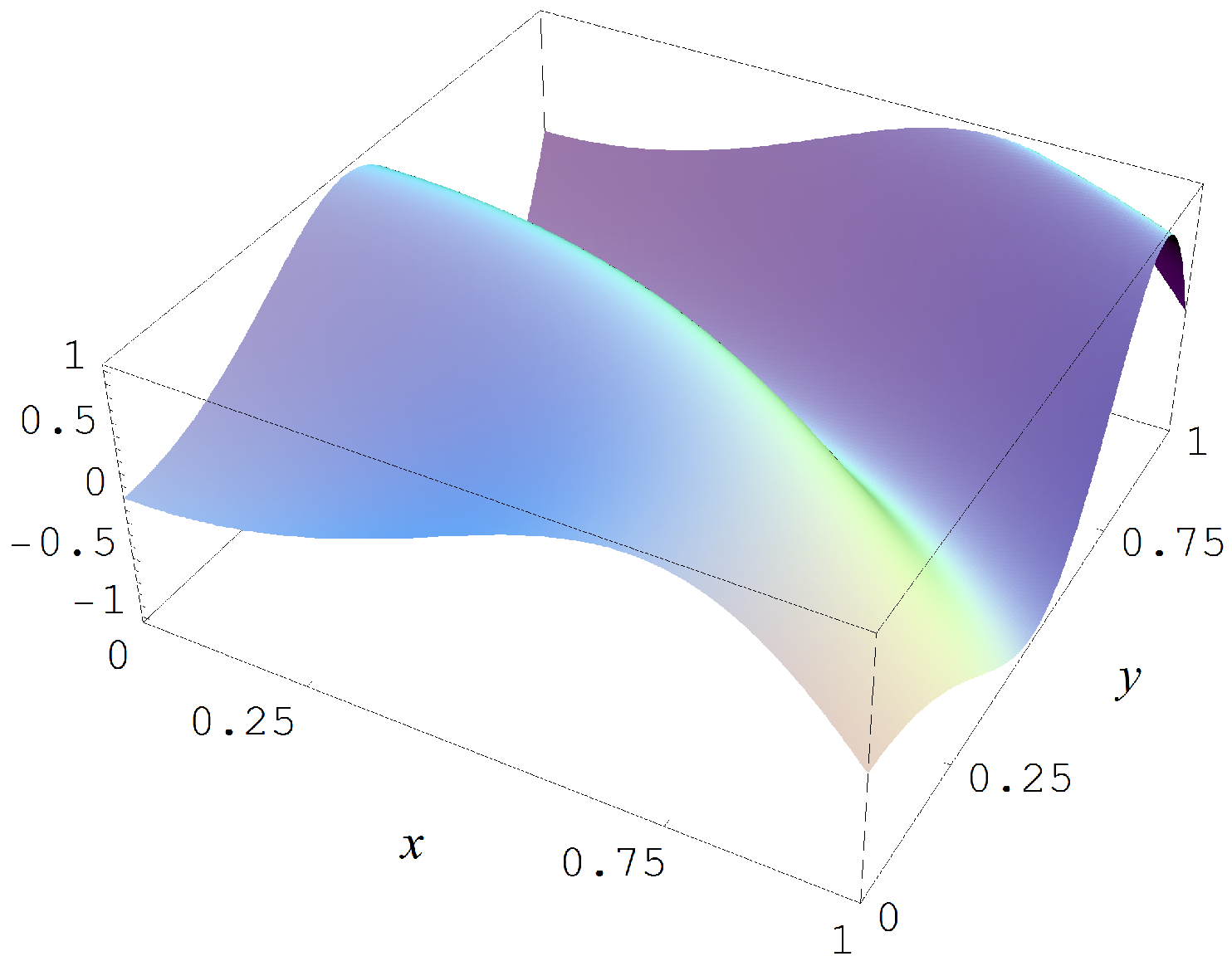
Figure A1.
Target function (A2).
Figure A1.
Target function (A2).
In Figure A2 some representative examples of large size data sets are shown for the different noise levels .
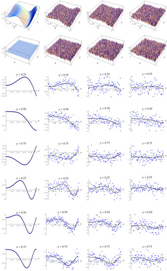

Figure A2.
Noisy data sampled from target function (A2). Columns correspond with noise levels , and 2, respectively. Rows correspond with noisy data, noisy data minus true target value, and cross sections of the target function and noisy data.
Figure A2.
Noisy data sampled from target function (A2). Columns correspond with noise levels , and 2, respectively. Rows correspond with noisy data, noisy data minus true target value, and cross sections of the target function and noisy data.
For it is found, Table A1, that the Ignorance, Manor, and BIC evidences are the most conservative of all the viable evidences in terms of the number of parameters m of the respective spline models. The Neeley and Constantineau evidences are slightly less conservative, as they choose for a model that is one order less conservative in terms of the number of parameters m, relatively to the Ignorance, Manor, and BIC evidences. The AIC evidence takes the high ground in that it is consistently less conservative in terms of the number of parameters m, relatively to the Ignorance, Manor, Neeley, Constantineau, and BIC evidences. Finally, the “sure thing” evidence just chooses the largest model available, thus, consistently (grossly) over-fitting the data. Also, it may be noted that in the absence of noise (i.e., ) all the evidences are in agreement in taking the model with the largest possible number of parameters; i.e., the model with a 7-by-7 partitioning, a polynomial order of , and a continuity order of .

Table A1.
C-spline models (geometry g, polynomial order d, continuity order r) and number of parameters m that were chosen by the discussed evidences, for and under Gaussian noise levels , and 2.
Table A1.
C-spline models (geometry g, polynomial order d, continuity order r) and number of parameters m that were chosen by the discussed evidences, for and under Gaussian noise levels , and 2.
| Evidences | Model 1 | Model 2 | Model 3 | Model 4 | ||||
|---|---|---|---|---|---|---|---|---|
| “Sure thing” (41) | 484 | 484 | 484 | 484 | ||||
| AIC (143) | 484 | 49 | 36 | 36 | ||||
| Neeley (127), Constantineau (130) | 484 | 36 | 25 | 25 | ||||
| Ignorance (127), Manor (127), BIC (135) | 484 | 36 | 25 | 16 | ||||
Data estimates: , , , and ; Data estimates: , , , and ; Data estimates: , , , and ; Data estimates: , , , and .
In Figure A3, Figure A4, Figure A5 and Figure A6, the fitted C-spline models are given per evidence (group), starting with the “sure thing” evidence and in descending order of liberalness in terms of the number of parameters m. In Figure A6 there is a possible instance of under-fitting for a noise level of (i.e., fourth column) by the model which is picked by the Ignorance, Manor, and BIC evidences.
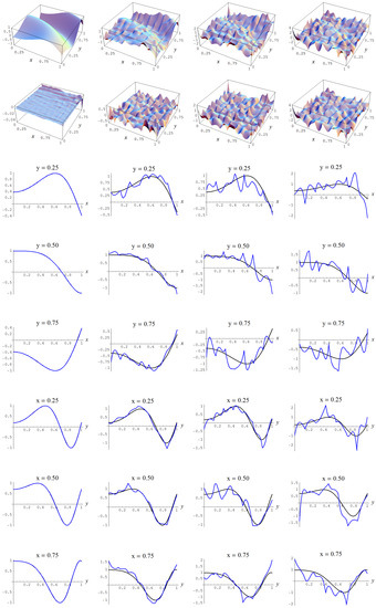
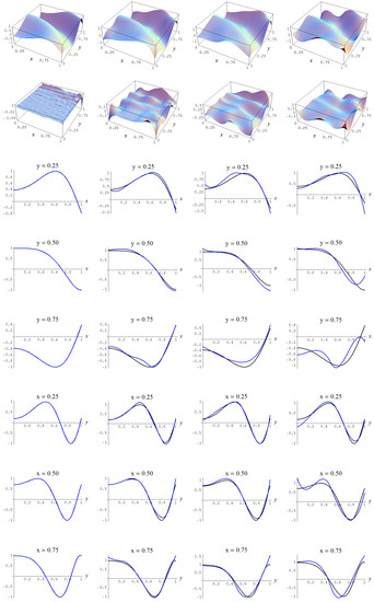
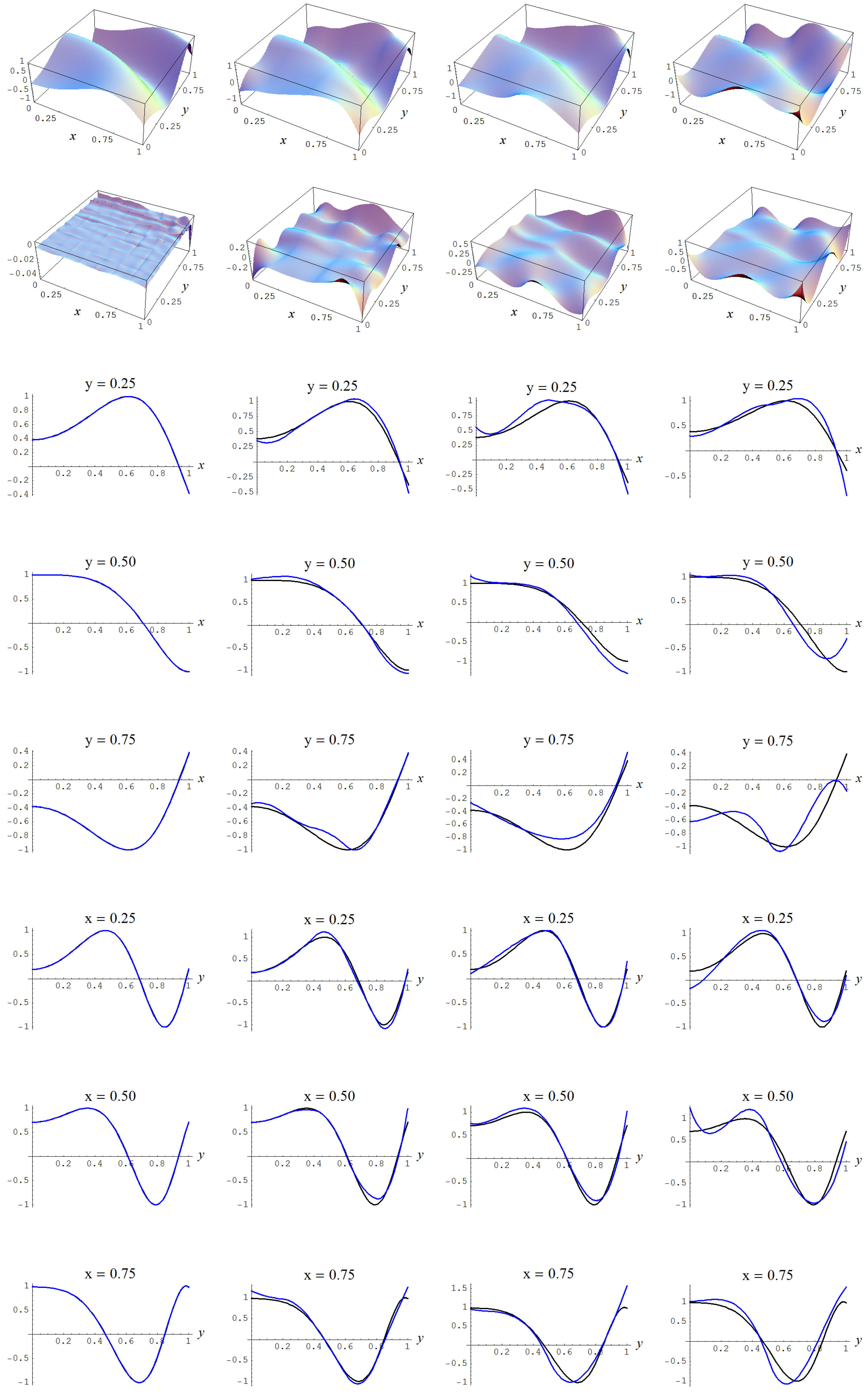
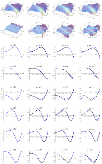
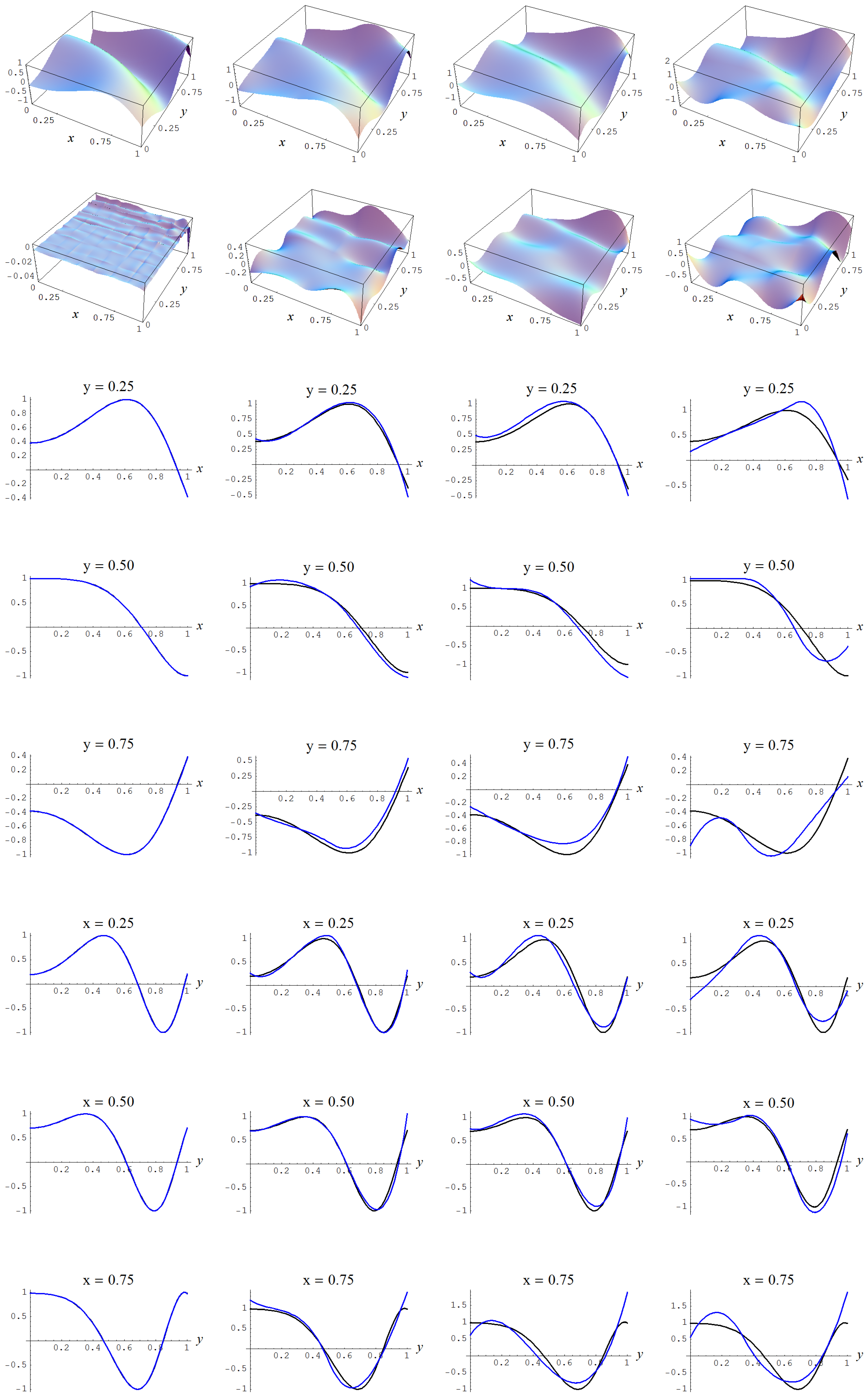
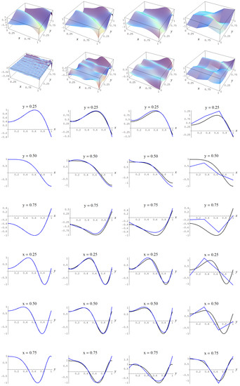
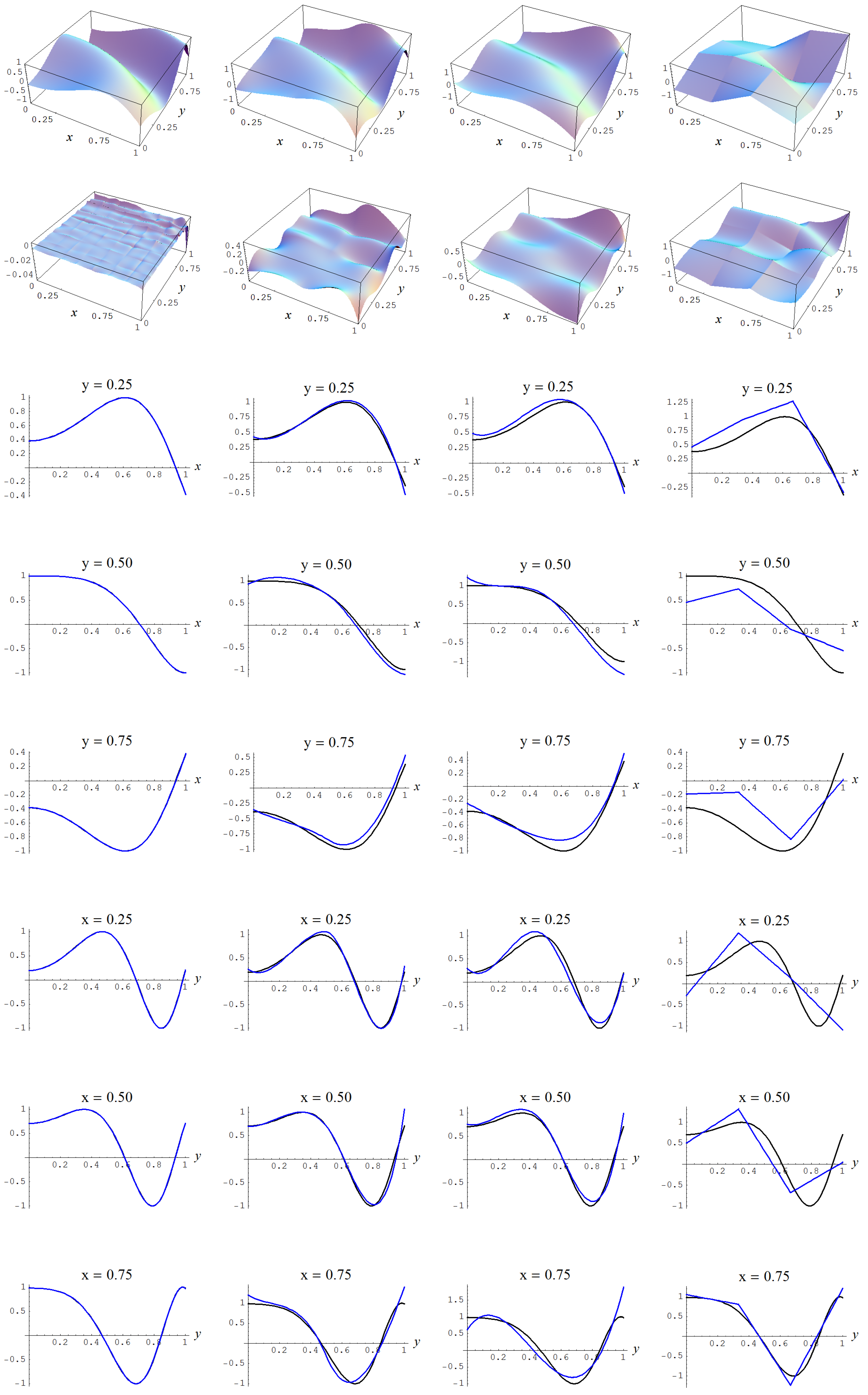
Figure A3.
Sample size and C-spline models of target function (A2) are picked by the “sure thing” evidence (41) for different noise levels. Columns correspond with noise levels , and 2, respectively. Rows correspond with spline model, residual of spline model relative to target function, and cross sections of spline model (blue) and target function (black).
Figure A4.
Sample size and C-spline models of target function (A2) are picked by the AIC evidence (143) for different noise levels. Columns correspond with noise levels , and 2, respectively. Rows correspond with spline model, residual of spline model relative to target function, and cross sections of spline model (blue) and target function (black).
Figure A5.
Sample size and C-spline models of target function (A2) are picked by the Neeley and the Constantineau evidences, (129) and (130), for different noise levels. Columns correspond with noise levels , and 2, respectively. Rows correspond with spline model, residual of spline model relative to target function, and cross sections of spline model (blue) and target function (black).
Figure A6.
Sample size and C-spline models of target function (A2) are picked by the Ignorance, Manor, and BIC evidences, (135), (127), and (128), for different noise levels. Columns correspond with noise levels , and 2, respectively. Rows correspond with spline model, residual of spline model relative to target function, and cross sections of spline model (blue) and target function (black).
In order to give the reader a more concrete sense of the discussed evidences, we give for the Gaussian noise level of the full output of the Bayesian model selection analysis in Table A2. It may be noted in these tables that the highest “sure thing” evidence must necessarily correspond with the lowest sample error standard deviation s, or, equivalently, the smallest sample error variance , since we have that this sample error variance, (152),
is an inverse root of the “sure thing” evidence (41). Likewise, let the sample variance be given as
where is the sample mean
then we have that the highest “sure thing” evidence must necessarily correspond with the highest R-square value, since we have that,
Stated differently, model selection based on R-square values is equivalent to model selection based on “sure thing” evidences (41).
Table A2.
Output model selection analysis for data sampled from target function (A2), sample size , and Gaussian error of ; given are (internally) ranked logarithms of the discussed evidences, ranked sample error standard deviations (from low to high) and R-square values, number of parameters m, and spline model specifications (geometry, polynomial-order, and continuity-order).
| Ignorance | Manor | Neeley | Constantineau | BIC | AIC | “Sure Thing” | Error Std | R-Square | m | Model Specs | |||||||||||
|---|---|---|---|---|---|---|---|---|---|---|---|---|---|---|---|---|---|---|---|---|---|
| 1 | −21,383 | 1 | −21,383 | 1 | −21,353 | 1 | −21,341 | 1 | −21,371 | 13 | −21,290 | 30 | −21,265 | 30 | 0.99 | 30 | 0.32 | 25 | 2 | 3 | 2 |
| 2 | −21,385 | 2 | −21,385 | 2 | −21,355 | 3 | −21,344 | 2 | −21,373 | 17 | −21,292 | 31 | −21,267 | 31 | 0.99 | 31 | 0.32 | 25 | 3 | 2 | 1 |
| 3 | −21,403 | 3 | −21,403 | 3 | −21,359 | 2 | −21,343 | 3 | −21,392 | 1 | −21,275 | 25 | −21,239 | 25 | 0.99 | 25 | 0.33 | 36 | 2 | 3 | 1 |
| 4 | −21,408 | 4 | −21,407 | 4 | −21,364 | 4 | −21,348 | 4 | −21,396 | 2 | −21,279 | 27 | −21,243 | 27 | 0.99 | 27 | 0.33 | 36 | 4 | 2 | 1 |
| 5 | −21,410 | 5 | −21,409 | 5 | −21,366 | 5 | −21,350 | 5 | −21,398 | 4 | −21,281 | 28 | −21,245 | 28 | 0.99 | 28 | 0.33 | 36 | 3 | 3 | 2 |
| 6 | −21,411 | 6 | −21,411 | 7 | −21,381 | 9 | −21,369 | 6 | −21,399 | 23 | −21,318 | 32 | −21,293 | 32 | 1.00 | 32 | 0.32 | 25 | 2 | 2 | 0 |
| 7 | −21,412 | 7 | −21,411 | 6 | −21,368 | 6 | −21,351 | 7 | −21,400 | 6 | −21,283 | 29 | −21,247 | 29 | 0.99 | 29 | 0.33 | 36 | 5 | 1 | 0 |
| 8 | −21,415 | 8 | −21,415 | 8 | −21,385 | 12 | −21,373 | 8 | −21,403 | 24 | −21,322 | 33 | −21,297 | 33 | 1.00 | 33 | 0.32 | 25 | 4 | 1 | 0 |
| 9 | −21,449 | 9 | −21,448 | 9 | −21,389 | 7 | −21,366 | 9 | −21,440 | 3 | −21,280 | 21 | −21,231 | 21 | 0.99 | 21 | 0.33 | 49 | 2 | 3 | 0 |
| 10 | −21,451 | 10 | −21,450 | 10 | −21,391 | 8 | −21,369 | 10 | −21,442 | 5 | −21,282 | 22 | −21,233 | 22 | 0.99 | 22 | 0.33 | 49 | 4 | 3 | 2 |
| 11 | −21,452 | 11 | −21,452 | 11 | −21,393 | 10 | −21,370 | 11 | −21,443 | 8 | −21,284 | 23 | −21,235 | 23 | 0.99 | 23 | 0.33 | 49 | 5 | 2 | 1 |
| 12 | −21,453 | 12 | −21,452 | 12 | −21,393 | 11 | −21,370 | 12 | −21,444 | 9 | −21,284 | 24 | −21,235 | 24 | 0.99 | 24 | 0.33 | 49 | 3 | 2 | 0 |
| 13 | −21,459 | 13 | −21,458 | 13 | −21,399 | 13 | −21,377 | 13 | −21,450 | 16 | −21,290 | 26 | −21,241 | 26 | 0.99 | 26 | 0.33 | 49 | 6 | 1 | 0 |
| 14 | −21,496 | 14 | −21,495 | 14 | −21,417 | 14 | −21,388 | 14 | −21,492 | 7 | −21,283 | 17 | −21,219 | 17 | 0.99 | 17 | 0.34 | 64 | 6 | 2 | 1 |
| 15 | −21,498 | 15 | −21,496 | 15 | −21,419 | 15 | −21,390 | 15 | −21,494 | 10 | −21,285 | 18 | −21,221 | 18 | 0.99 | 18 | 0.34 | 64 | 3 | 3 | 1 |
| 16 | −21,502 | 16 | −21,501 | 16 | −21,423 | 16 | −21,394 | 16 | −21,498 | 11 | −21,289 | 19 | −21,225 | 19 | 0.99 | 19 | 0.34 | 64 | 5 | 3 | 2 |
| 17 | −21,502 | 17 | −21,501 | 17 | −21,424 | 17 | −21,394 | 17 | −21,498 | 12 | −21,289 | 20 | −21,225 | 20 | 0.99 | 20 | 0.34 | 64 | 7 | 1 | 0 |
| 18 | −21,508 | 20 | −21,508 | 23 | −21,489 | 27 | −21,482 | 20 | −21,498 | 34 | −21,446 | 36 | −21,430 | 34 | 1.03 | 36 | 0.28 | 16 | 1 | 3 | 0 |
| 19 | −21,508 | 19 | −21,508 | 22 | −21,489 | 26 | −21,482 | 19 | −21,498 | 33 | −21,446 | 35 | -21,430 | 35 | 1.03 | 35 | 0.28 | 16 | 1 | 3 | 1 |
| 20 | −21,508 | 18 | −21,508 | 21 | −21,489 | 25 | −21,482 | 18 | −21,498 | 32 | −21,446 | 34 | −21,430 | 36 | 1.03 | 34 | 0.28 | 16 | 1 | 3 | 2 |
| 21 | −21,509 | 21 | −21,508 | 24 | −21,489 | 28 | −21,482 | 21 | −21,498 | 35 | −21,446 | 37 | −21,430 | 37 | 1.03 | 37 | 0.28 | 16 | 2 | 2 | 1 |
| 22 | −21,523 | 22 | −21,523 | 28 | −21,504 | 29 | −21,497 | 22 | −21,513 | 36 | −21,461 | 38 | −21,445 | 38 | 1.03 | 38 | 0.27 | 16 | 3 | 1 | 0 |
| 23 | −21,550 | 23 | −21,549 | 18 | −21,451 | 18 | −21,414 | 23 | −21,554 | 14 | −21,290 | 13 | −21,209 | 13 | 0.98 | 13 | 0.34 | 81 | 7 | 2 | 1 |
| 24 | −21,550 | 24 | −21,549 | 19 | −21,451 | 19 | −21,414 | 24 | −21,554 | 15 | −21,290 | 14 | −21,209 | 14 | 0.98 | 14 | 0.34 | 81 | 4 | 2 | 0 |
| 25 | −21,559 | 25 | −21,558 | 20 | −21,460 | 20 | −21,423 | 25 | −21,563 | 18 | −21,299 | 16 | −21,218 | 16 | 0.99 | 16 | 0.34 | 81 | 6 | 3 | 2 |
| 26 | −21,613 | 26 | −21,611 | 25 | −21,491 | 21 | −21,445 | 26 | −21,628 | 19 | −21,302 | 11 | −21,202 | 11 | 0.98 | 11 | 0.34 | 100 | 3 | 3 | 0 |
| 27 | −21,620 | 27 | −21,618 | 26 | −21,497 | 22 | −21,451 | 27 | −21,634 | 21 | −21,308 | 12 | −21,208 | 12 | 0.98 | 12 | 0.34 | 100 | 4 | 3 | 1 |
| 28 | −21,622 | 28 | −21,621 | 27 | −21,500 | 23 | −21,454 | 28 | −21,637 | 22 | −21,311 | 15 | −21,211 | 15 | 0.98 | 15 | 0.34 | 100 | 7 | 3 | 2 |
| 29 | −21,663 | 29 | −21,662 | 33 | −21,652 | 35 | −21,648 | 29 | −21,655 | 39 | −21,626 | 39 | −21,617 | 39 | 1.07 | 39 | 0.22 | 9 | 2 | 1 | 0 |
| 30 | −21,674 | 30 | −21,671 | 29 | −21,525 | 24 | −21,469 | 30 | −21,702 | 20 | −21,308 | 9 | −21,187 | 9 | 0.98 | 9 | 0.35 | 121 | 5 | 2 | 0 |
| 31 | −21,714 | 32 | −21,714 | 37 | −21,704 | 39 | −21,700 | 32 | −21,707 | 41 | −21,678 | 41 | −21,669 | 40 | 1.08 | 41 | 0.21 | 9 | 1 | 2 | 0 |
| 32 | −21,714 | 31 | −21,714 | 36 | −21,704 | 38 | −21,700 | 31 | −21,707 | 40 | −21,678 | 40 | −21,669 | 41 | 1.08 | 40 | 0.21 | 9 | 1 | 2 | 1 |
| 33 | −21,756 | 33 | −21,753 | 30 | −21,580 | 30 | −21,513 | 33 | −21,802 | 26 | −21,333 | 10 | −21,189 | 10 | 0.98 | 10 | 0.34 | 144 | 5 | 3 | 1 |
| 34 | −21,816 | 34 | −21,813 | 31 | −21,609 | 31 | −21,530 | 34 | −21,882 | 25 | −21,332 | 5 | −21,163 | 5 | 0.97 | 5 | 0.35 | 169 | 6 | 2 | 0 |
| 35 | −21,829 | 35 | −21,826 | 32 | −21,622 | 32 | −21,543 | 35 | −21,895 | 27 | −21,344 | 7 | −21,175 | 7 | 0.98 | 7 | 0.35 | 169 | 4 | 3 | 0 |
| 36 | −21,919 | 36 | −21,916 | 34 | −21,679 | 34 | −21,588 | 36 | −22,010 | 29 | −21,372 | 8 | −21,176 | 8 | 0.98 | 8 | 0.35 | 196 | 6 | 3 | 1 |
| 37 | −21,963 | 37 | −21,959 | 35 | −21,686 | 33 | −21,580 | 38 | −22,080 | 28 | −21,347 | 3 | −21,122 | 3 | 0.97 | 3 | 0.36 | 225 | 7 | 2 | 0 |
| 38 | −22,066 | 38 | −22,066 | 41 | −22,061 | 42 | −22,060 | 37 | −22,062 | 42 | −22,049 | 42 | −22,045 | 42 | 1.16 | 42 | 0.08 | 4 | 1 | 1 | 0 |
| 39 | −22,085 | 39 | −22,081 | 38 | −21,771 | 36 | −21,651 | 39 | −22,236 | 30 | −21,402 | 4 | −21,146 | 4 | 0.97 | 4 | 0.36 | 256 | 5 | 3 | 0 |
| 40 | −22,105 | 40 | −22,101 | 39 | −21,792 | 37 | −21,672 | 40 | −22,257 | 31 | −21,423 | 6 | −21,167 | 6 | 0.98 | 6 | 0.35 | 256 | 7 | 3 | 1 |
| 41 | −22,378 | 41 | −22,371 | 40 | −21,934 | 40 | −21,764 | 41 | −22,650 | 37 | −21,473 | 2 | −21,112 | 2 | 0.96 | 2 | 0.36 | 361 | 6 | 3 | 0 |
| 42 | −22,712 | 42 | −22,704 | 42 | −22,117 | 41 | −21,887 | 42 | −23,145 | 38 | −21,567 | 1 | −21,083 | 1 | 0.96 | 1 | 0.37 | 484 | 7 | 3 | 0 |
For N = 10,000 the same pattern can be discerned as for , Table A3. The Ignorance, Manor, and BIC evidences are the most conservative of all the viable evidences in terms of the number of parameters m of the respective spline models. The Neeley and Constantineau evidences are slightly less conservative, as they choose for a model that is one order less conservative in terms of the number of parameters m, relatively to the Ignorance, Manor, and BIC evidences. The AIC evidence takes the high ground in that it is consistently less conservative in terms of the number of parameters m, relatively to the Ignorance, Manor, Neeley, Constantineau, and BIC evidences. Finally, the “sure thing” evidence just chooses the largest model available, thus, consistently (grossly) over-fitting the data. And it may again be noted that in the absence of noise (i.e., ) all the evidences are in agreement in taking the model with the largest possible number of parameters.
Table A3.
C-spline models (geometry g, polynomial order d, continuity order r) and number of parameters m that were chosen by the discussed evidences, for and under Gaussian noise levels , and 2.
Table A3.
C-spline models (geometry g, polynomial order d, continuity order r) and number of parameters m that were chosen by the discussed evidences, for and under Gaussian noise levels , and 2.
| Evidences | Model | Model | Model | Model | ||||
|---|---|---|---|---|---|---|---|---|
| “Sure thing” (41) | 484 | 484 | 484 | 484 | ||||
| AIC (143) | 484 | 64 | 49 | 36 | ||||
| Neeley (127), Constantineau (130) | 484 | 49 | 36 | 25 | ||||
| Ignorance (127), Manor (127), BIC (135) | 484 | 36 | 36 | 25 | ||||
Data estimates: , , , and ; Data estimates: , , , and ; Data estimates: , , , and ; Data estimates: , , , and .
In Figure A7, Figure A8, Figure A9 and Figure A10, the fitted C-spline models are given per evidence (group), starting with the “sure thing” evidence and in descending order of liberalness in terms of the number of parameters m. In Figure A8 there is a possible instance of over-fitting for a noise level (i.e., column 3) by the model which is picked by the AIC evidence. Also, again in order to give the reader a more concrete sense of the discussed evidences, we give for the Gaussian noise level of the full output of the Bayesian model selection analysis in Table A4.
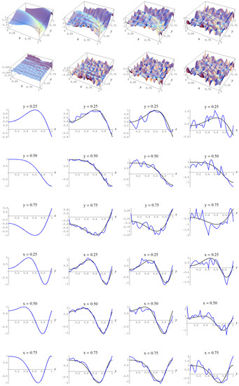

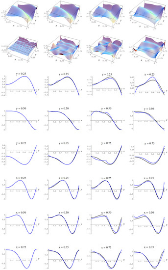
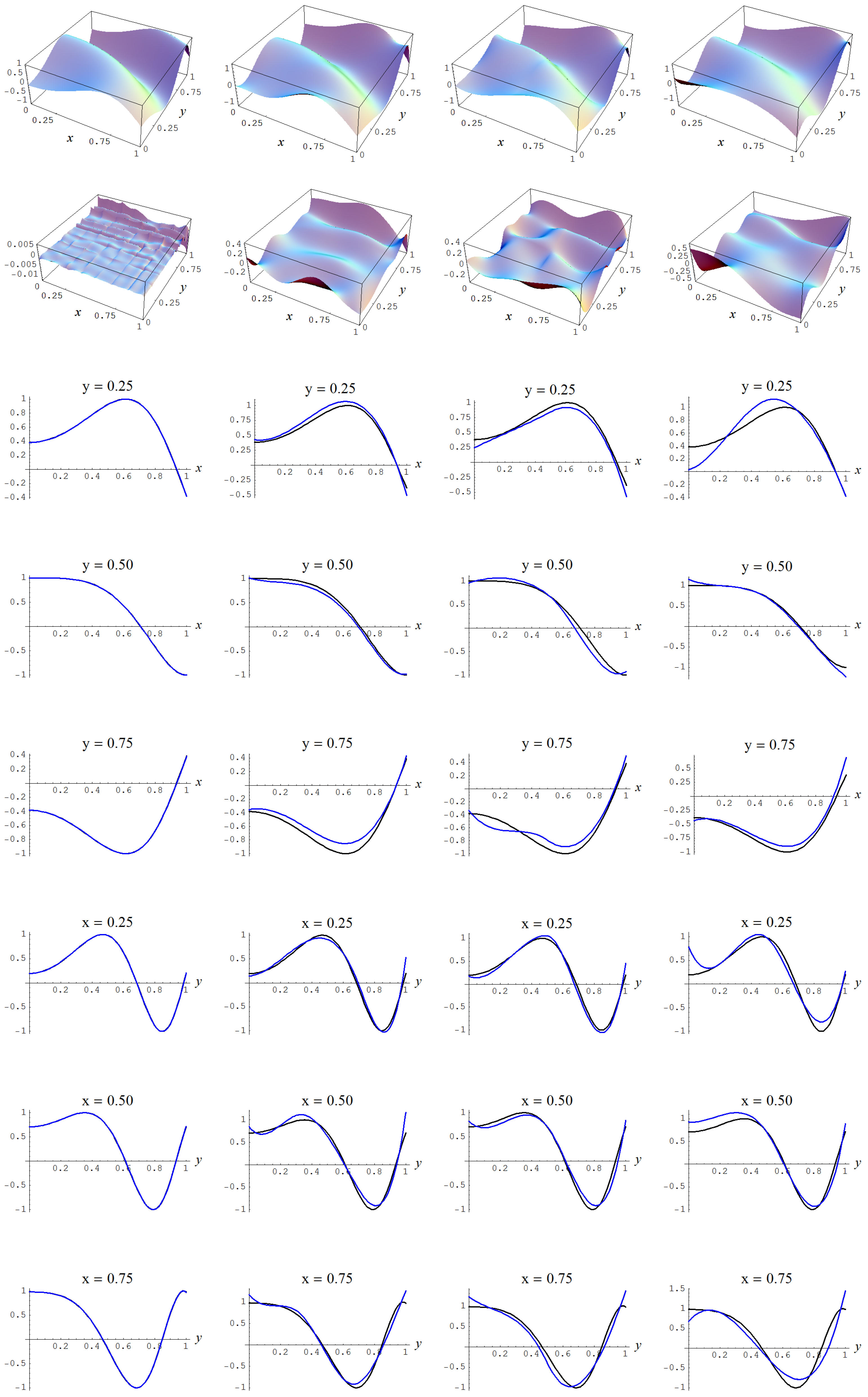
Figure A7.
Sample size 10,000 and C-spline models of target function (A2) are picked by the “sure thing” evidence (41) for different noise levels. Columns correspond with noise levels , and 2, respectively. Rows correspond with spline model, residual of spline model relative to target function, and cross sections of spline model (blue) and target function (black).
Figure A8.
Sample size 10,000 and C-spline models of target function (A2) are picked by the AIC evidence (143) for different noise levels. Columns correspond with noise levels , and 2, respectively. Rows correspond with spline model, residual of spline model relative to target function, and cross sections of spline model (blue) and target function (black).
Figure A9.
Sample size 10,000 and C-spline models of target function (A2) are picked by the Neeley and the Constantineau evidences, (129) and (130), for different noise levels. Columns correspond with noise levels , and 2, respectively. Rows correspond with spline model, residual of spline model relative to target function, and cross sections of spline model (blue) and target function (black).
Figure A10.
Sample size N = 10,000 and C-spline models of target function (A2) are picked by the Ignorance, Manor, and Bayesian Information Criterion (BIC) evidences, (135), (127), and (128), for different noise levels. Columns correspond with noise levels , and 2, respectively. Rows correspond with spline model, residual of spline model relative to target function, and cross sections of spline model (blue) and target function (black).
Table A4.
Output model selection analysis for data sampled from target function (A2), sample size N = 10,000, and Gaussian error of ; given are (internally) ranked logarithms of the discussed evidences, ranked sample error standard deviations (from low to high) and R-square values, number of parameters m, and spline model specifications (geometry, polynomial-order, and continuity-order).
| Ignorance | Manor | Neeley | Constantineau | BIC | AIC | “Sure Thing” | Error Std | R-Square | m | Model Specs | |||||||||||
|---|---|---|---|---|---|---|---|---|---|---|---|---|---|---|---|---|---|---|---|---|---|
| 1 | −46,177 | 1 | −46,176 | 1 | −46,132 | 1 | −46,115 | 1 | −46,164 | 4 | −46,035 | 26 | −45,999 | 26 | 0.99 | 26 | 0.32 | 36 | 2 | 3 | 1 |
| 2 | −46,179 | 2 | −46,179 | 4 | −46,148 | 5 | −46,137 | 2 | −46,167 | 21 | −46,076 | 30 | −46,051 | 30 | 1.00 | 30 | 0.31 | 25 | 2 | 3 | 2 |
| 3 | −46,181 | 3 | −46,181 | 5 | −46,150 | 8 | −46,138 | 3 | −46,168 | 22 | −46,078 | 31 | −46,053 | 31 | 1.00 | 31 | 0.31 | 25 | 3 | 2 | 1 |
| 4 | −46,182 | 4 | −46,182 | 2 | −46,137 | 2 | −46,121 | 4 | −46,169 | 10 | −46,040 | 27 | −46,004 | 27 | 1.00 | 27 | 0.32 | 36 | 4 | 2 | 1 |
| 5 | −46,186 | 5 | −46,186 | 3 | −46,141 | 3 | −46,125 | 5 | −46,174 | 12 | −46,044 | 28 | −46,008 | 28 | 1.00 | 28 | 0.32 | 36 | 3 | 3 | 2 |
| 6 | −46,203 | 6 | −46,203 | 6 | −46,158 | 10 | −46,142 | 6 | −46,191 | 16 | −46,061 | 29 | −46,025 | 29 | 1.00 | 29 | 0.31 | 36 | 5 | 1 | 0 |
| 7 | −46,220 | 7 | −46,219 | 7 | −46,159 | 4 | −46,137 | 7 | −46,210 | 1 | −46,033 | 21 | −45,984 | 21 | 0.99 | 21 | 0.32 | 49 | 2 | 3 | 0 |
| 8 | −46,220 | 8 | −46,220 | 8 | −46,159 | 6 | −46,137 | 8 | −46,210 | 2 | −46,034 | 22 | −45,985 | 22 | 0.99 | 22 | 0.32 | 49 | 4 | 3 | 2 |
| 9 | −46,221 | 9 | −46,221 | 9 | −46,160 | 7 | −46,138 | 9 | −46,211 | 3 | −46,034 | 23 | −45,985 | 23 | 0.99 | 23 | 0.32 | 49 | 5 | 2 | 1 |
| 10 | −46,223 | 10 | −46,223 | 10 | −46,162 | 9 | −46,140 | 10 | −46,214 | 5 | −46,037 | 24 | −45,988 | 24 | 0.99 | 24 | 0.32 | 49 | 3 | 2 | 0 |
| 11 | −46,226 | 11 | −46,225 | 11 | −46,164 | 11 | −46,142 | 11 | −46,216 | 8 | −46,039 | 25 | −45,990 | 25 | 0.99 | 25 | 0.32 | 49 | 6 | 1 | 0 |
| 12 | −46,237 | 12 | −46,237 | 16 | −46,206 | 16 | −46,195 | 12 | −46,225 | 27 | −46,135 | 32 | −46,110 | 32 | 1.01 | 32 | 0.30 | 25 | 2 | 2 | 0 |
| 13 | −46,239 | 13 | −46,239 | 17 | −46,208 | 17 | −46,197 | 13 | −46,226 | 28 | −46,136 | 33 | −46,111 | 33 | 1.01 | 33 | 0.30 | 25 | 4 | 1 | 0 |
| 14 | −46,274 | 14 | −46,274 | 12 | −46,194 | 12 | −46,165 | 14 | −46,269 | 6 | −46,038 | 17 | −45,974 | 17 | 0.99 | 17 | 0.32 | 64 | 5 | 3 | 2 |
| 15 | −46,274 | 15 | −46,274 | 13 | −46,194 | 13 | −46,165 | 15 | −46,269 | 7 | −46,038 | 18 | −45,974 | 18 | 0.99 | 18 | 0.32 | 64 | 6 | 2 | 1 |
| 16 | −46,275 | 16 | −46,275 | 14 | −46,195 | 14 | −46,166 | 16 | −46,270 | 9 | −46,039 | 19 | −45,975 | 19 | 0.99 | 19 | 0.32 | 64 | 3 | 3 | 1 |
| 17 | −46,279 | 17 | −46,278 | 15 | −46,199 | 15 | −46,170 | 17 | −46,274 | 11 | −46,043 | 20 | −45,979 | 20 | 0.99 | 20 | 0.32 | 64 | 7 | 1 | 0 |
| 18 | −46,335 | 18 | −46,335 | 18 | −46,234 | 18 | −46,197 | 18 | −46,338 | 13 | −46,046 | 13 | −45,965 | 13 | 0.99 | 13 | 0.32 | 81 | 7 | 2 | 1 |
| 19 | −46,337 | 19 | −46,337 | 19 | −46,237 | 19 | −46,200 | 19 | −46,340 | 14 | −46,048 | 15 | −45,967 | 15 | 0.99 | 15 | 0.32 | 81 | 4 | 2 | 0 |
| 20 | −46,340 | 20 | −46,339 | 20 | −46,239 | 20 | −46,202 | 20 | −46,342 | 15 | −46,050 | 16 | −45,969 | 16 | 0.99 | 16 | 0.32 | 81 | 6 | 3 | 2 |
| 21 | −46,409 | 21 | −46,409 | 21 | −46,285 | 21 | −46,239 | 21 | −46,422 | 17 | −46,062 | 11 | −45,962 | 11 | 0.99 | 11 | 0.32 | 100 | 3 | 3 | 0 |
| 22 | −46,410 | 22 | −46,409 | 22 | −46,285 | 22 | −46,240 | 22 | −46,423 | 18 | −46,062 | 12 | −45,962 | 12 | 0.99 | 12 | 0.32 | 100 | 4 | 3 | 1 |
| 23 | −46,413 | 23 | −46,412 | 23 | −46,288 | 23 | −46,243 | 23 | −46,426 | 19 | −46,066 | 14 | −45,966 | 14 | 0.99 | 14 | 0.32 | 100 | 7 | 3 | 2 |
| 24 | −46,479 | 26 | −46,479 | 30 | −46,459 | 32 | −46,452 | 26 | −46,468 | 36 | −46,410 | 36 | −46,394 | 34 | 1.03 | 36 | 0.26 | 16 | 1 | 3 | 0 |
| 25 | −46,479 | 25 | −46,479 | 29 | −46,459 | 31 | −46,452 | 25 | −46,468 | 35 | −46,410 | 35 | −46,394 | 35 | 1.03 | 35 | 0.26 | 16 | 1 | 3 | 1 |
| 26 | −46,479 | 24 | −46,479 | 28 | −46,459 | 30 | −46,452 | 24 | −46,468 | 34 | −46,410 | 34 | −46,394 | 36 | 1.03 | 34 | 0.26 | 16 | 1 | 3 | 2 |
| 27 | −46,479 | 27 | −46,479 | 24 | −46,328 | 24 | −46,274 | 29 | −46,506 | 20 | −46,070 | 10 | −45,949 | 10 | 0.99 | 10 | 0.32 | 121 | 5 | 2 | 0 |
| 28 | −46,482 | 28 | −46,482 | 31 | −46,462 | 33 | −46,456 | 27 | −46,472 | 37 | −46,414 | 37 | −46,398 | 37 | 1.04 | 37 | 0.26 | 16 | 2 | 2 | 1 |
| 29 | −46,500 | 29 | −46,499 | 32 | −46,480 | 34 | −46,473 | 28 | −46,489 | 38 | −46,431 | 38 | −46,415 | 38 | 1.04 | 38 | 0.26 | 16 | 3 | 1 | 0 |
| 30 | −46,566 | 30 | −46,565 | 25 | −46,386 | 25 | −46,321 | 30 | −46,610 | 23 | −46,090 | 9 | −45,946 | 9 | 0.99 | 9 | 0.32 | 144 | 5 | 3 | 1 |
| 31 | −46,636 | 31 | −46,635 | 26 | −46,425 | 26 | −46,348 | 31 | −46,700 | 24 | −46,091 | 5 | −45,922 | 5 | 0.99 | 5 | 0.33 | 169 | 6 | 2 | 0 |
| 32 | −46,647 | 32 | −46,647 | 27 | −46,437 | 27 | −46,360 | 32 | −46,712 | 25 | −46,103 | 7 | −45,934 | 7 | 0.99 | 7 | 0.33 | 169 | 4 | 3 | 0 |
| 33 | −46,756 | 33 | −46,755 | 33 | −46,512 | 28 | −46,423 | 36 | −46,845 | 29 | −46,139 | 8 | −45,943 | 8 | 0.99 | 8 | 0.32 | 196 | 6 | 3 | 1 |
| 34 | −46,758 | 34 | −46,758 | 37 | −46,747 | 38 | −46,744 | 33 | −46,751 | 39 | −46,718 | 39 | −46,709 | 39 | 1.07 | 39 | 0.21 | 9 | 2 | 1 | 0 |
| 35 | −46,817 | 35 | −46,817 | 34 | −46,537 | 29 | −46,434 | 37 | −46,934 | 26 | −46,123 | 3 | −45,898 | 3 | 0.98 | 3 | 0.33 | 225 | 7 | 2 | 0 |
| 36 | −46,846 | 37 | −46,846 | 40 | −46,835 | 41 | −46,831 | 35 | −46,839 | 41 | −46,806 | 41 | −46,797 | 40 | 1.08 | 41 | 0.20 | 9 | 1 | 2 | 0 |
| 37 | −46,846 | 36 | −46,846 | 39 | −46,835 | 40 | −46,831 | 34 | −46,839 | 40 | −46,806 | 40 | −46,797 | 41 | 1.08 | 40 | 0.20 | 9 | 1 | 2 | 1 |
| 38 | −46,939 | 38 | −46,938 | 35 | −46,620 | 35 | −46,503 | 38 | −47,088 | 30 | −46,165 | 4 | −45,909 | 4 | 0.99 | 4 | 0.33 | 256 | 5 | 3 | 0 |
| 39 | −46,955 | 39 | −46,954 | 36 | −46,636 | 36 | −46,520 | 39 | −47,105 | 31 | −46,182 | 6 | −45,926 | 6 | 0.99 | 6 | 0.33 | 256 | 7 | 3 | 1 |
| 40 | −47,261 | 40 | −47,259 | 38 | −46,810 | 37 | −46,644 | 41 | −47,530 | 32 | −46,229 | 2 | −45,868 | 2 | 0.98 | 2 | 0.33 | 361 | 6 | 3 | 0 |
| 41 | −47,521 | 41 | −47,521 | 42 | −47,516 | 42 | −47,515 | 40 | −47,517 | 42 | −47,502 | 42 | −47,498 | 42 | 1.16 | 42 | 0.08 | 4 | 1 | 1 | 0 |
| 42 | −47,648 | 42 | −47,646 | 41 | −47,044 | 39 | −46,821 | 42 | −48,079 | 33 | −46,334 | 1 | −45,850 | 1 | 0.98 | 1 | 0.34 | 484 | 7 | 3 | 0 |
In closing, note that for both and the cruelly realistic evidences (127)–(129), have been helped by estimating , , , and directly from the observed dependent variable y. So, if we penalize the computed evidences with a multiplication factor of , in order to compensate (see Section 5 of [3]) for the non-conservativeness of the data estimates of , , , and , it is found for N = 10,000 and that the Neely evidence will become one order of magnitude more conservative, as it picks the same model as the Ignorance, Manor, and BIC evidences, while at the same time we have that for N = 10,000 and the Ignorance and Manor evidences become one order of magnitude more conservative, thus, leaving the BIC evidence behind, as they choose the C-spline model , which has parameters.
Appendix A.2. Monte Carlo Study 2
In the second Monte Carlo study we sample from the target function
which is shown in Figure A11. The sampling in this second study is done with sample size N = 15,000, with Gaussian noise levels of , and 2, and multiplication factors of 1 and 10, respectively, for the data estimates of , , , and . The evidences must now choose amongst 78 models with parameters.
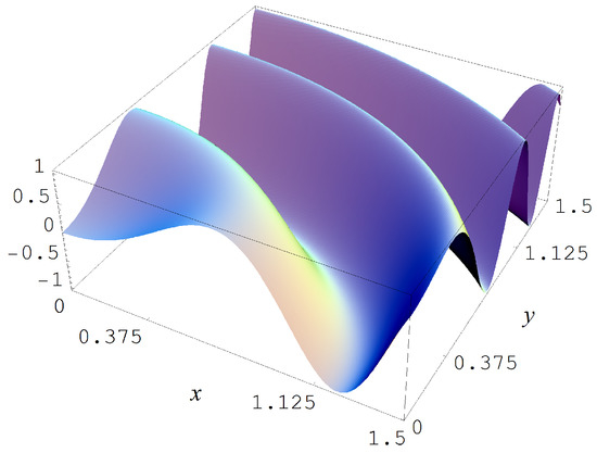
Figure A11.
Target function (A7).
Figure A11.
Target function (A7).
In Figure A12 some representative examples of large size data sets are shown for the different noise levels .
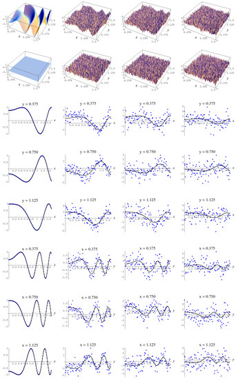
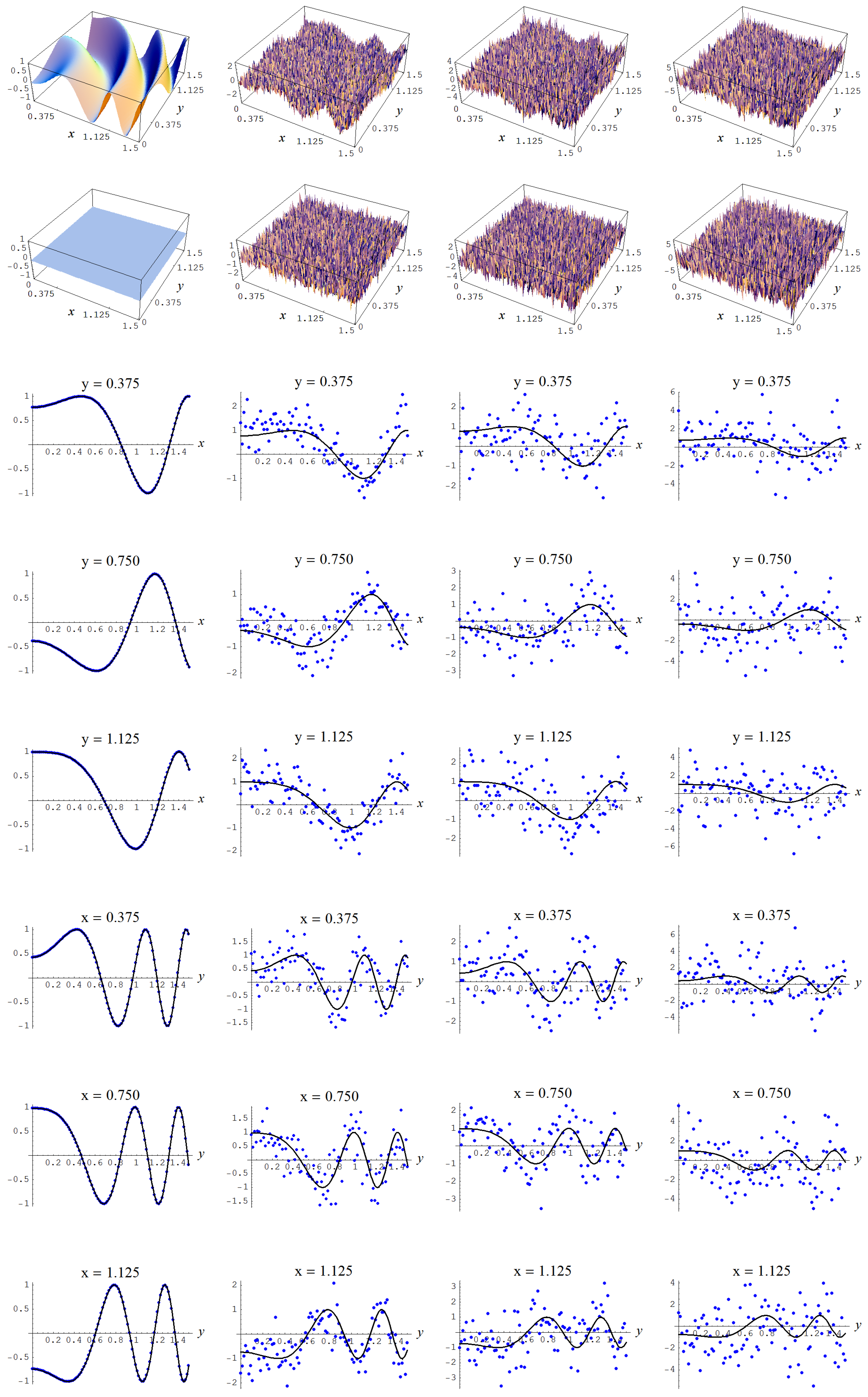
Figure A12.
Noisy data sampled from target function (A2). Columns correspond with noise levels , and 2, respectively. Rows correspond with noisy data, noisy data minus true target value, and cross sections of the target function and noisy data.
Figure A12.
Noisy data sampled from target function (A2). Columns correspond with noise levels , and 2, respectively. Rows correspond with noisy data, noisy data minus true target value, and cross sections of the target function and noisy data.
For a multiplication factor of 1, or, equivalently, a straightforward data-estimate of the characteristics of the dependent variable y, it is found, Table A5, that the Ignorance, Manor, Neeley, and BIC evidences become conservative in the absence of measurement error (i.e., ), as they choose a model with parameters, rather than the model with the maximum number of parameters which is preferred by the Constantineau, AIC, and “sure thing” evidences. Stated differently, the penalizing of an increase of parameters by the Occam factors the Ignorance, Manor, Neeley, and BIC evidences outweighs the gains in goodness of fit of said parameters.
Table A5.
C-spline models (geometry g, polynomial order d, continuity order r) and number of parameters m that were chosen by the discussed evidences, for under Gaussian noise levels , and 2, and a multiplication factor of 1 for the estimates of the characteristics of the dependent variable y.
Table A5.
C-spline models (geometry g, polynomial order d, continuity order r) and number of parameters m that were chosen by the discussed evidences, for under Gaussian noise levels , and 2, and a multiplication factor of 1 for the estimates of the characteristics of the dependent variable y.
| Evidences | Model | Model | Model | Model | ||||
|---|---|---|---|---|---|---|---|---|
| “Sure thing” (41) | 1600 | 1600 | 1600 | 1600 | ||||
| AIC (143) | 1600 | 196 | 144 | 121 | ||||
| Constantineau (130) | 1600 | 144 | 121 | 100 | ||||
| Neeley (127) | 625 | 144 | 121 | 100 | ||||
| Ignorance (127), Manor (127), | ||||||||
| BIC (135) | 625 | 144 | 100 | 64 | ||||
Data estimates times 1: , , , and ; Data estimates times 1: , , , and ; Data estimates times 1: , , , and ; Data estimates times 1: , , , and .
Apart from this deviation, we have that the pattern of model choices is roughly the same as observed in the first Monte Carlo study. The Ignorance, Manor, and BIC evidences are the most conservative of all the viable evidences in terms of the number of parameters m of the respective spline models. The Neeley and Constantineau evidences are slightly less conservative, as they choose both for and a model that is one order less conservative in terms of the number of parameters m, relatively to the Ignorance, Manor, and BIC evidences. The AIC evidence takes the high ground in that it is consistently less conservative in terms of the number of parameters m, relatively to the Ignorance, Manor, Neeley, Constantineau, and BIC evidences. Finally, the “sure thing” evidence just chooses the largest model available, thus, consistently (grossly) over-fitting the data.
In Figure A13, Figure A14, Figure A15, Figure A16 and Figure A17, the fitted C-spline models are given per evidence (group), starting with the “sure thing” evidence and in descending order of liberalness in terms of the number of parameters m. In Figure A17 there is a possible instance of under-fitting for a noise level (i.e., column 4) by the model which is picked by the Ignorance, Manor, and BIC evidences.
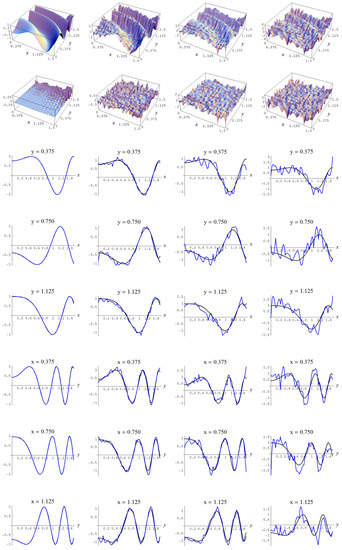
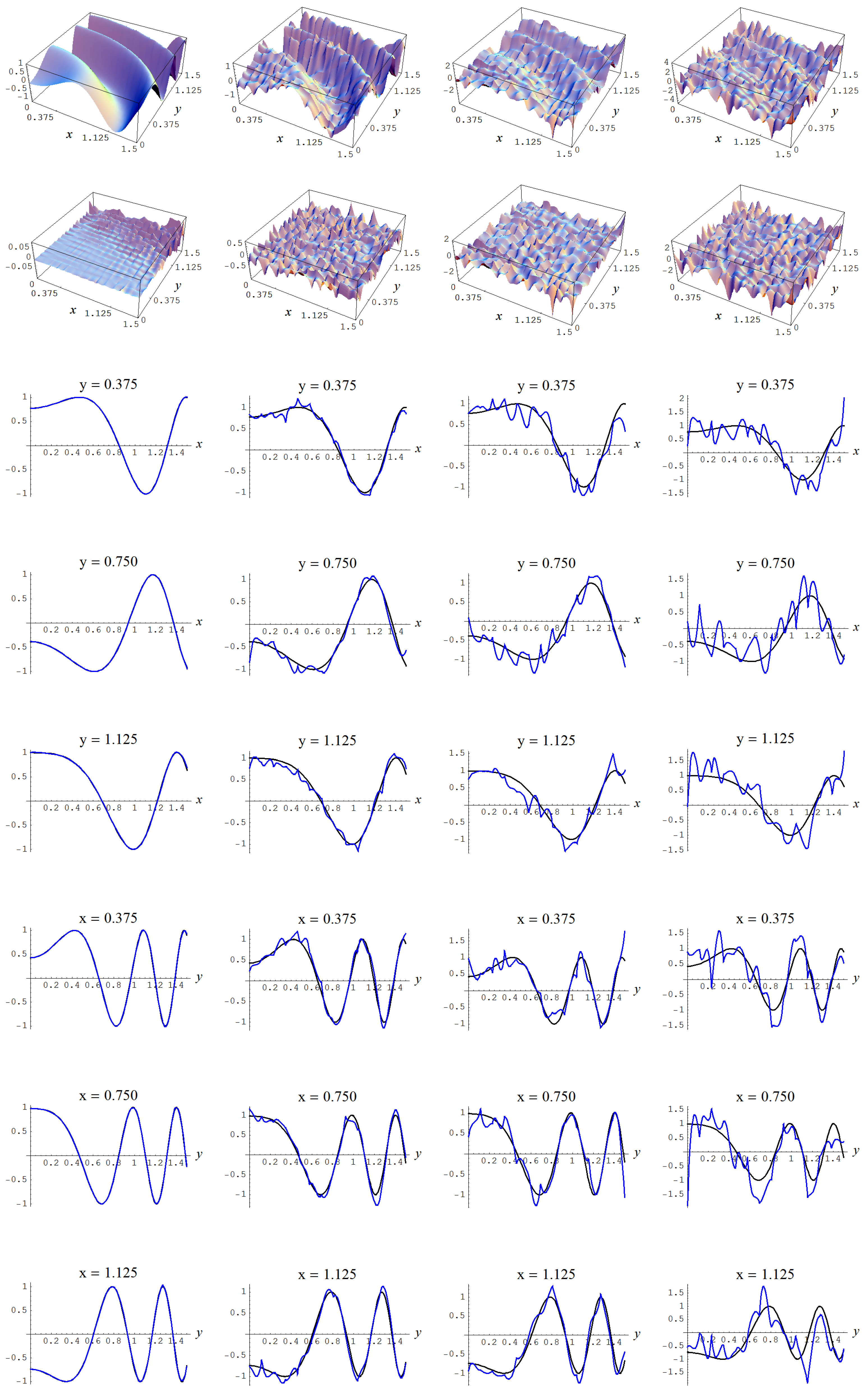
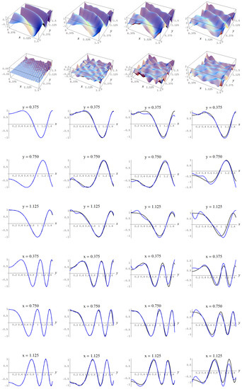
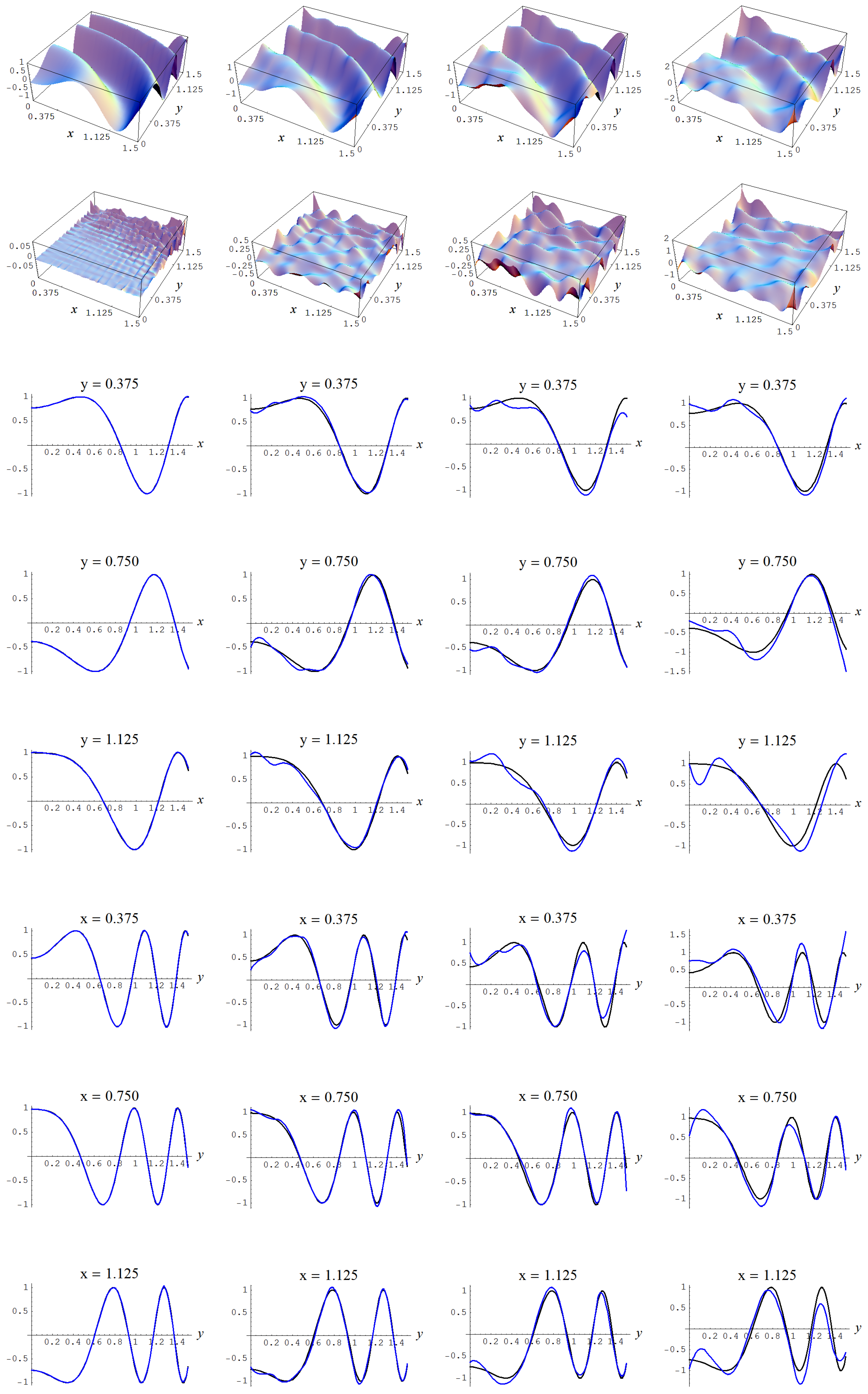
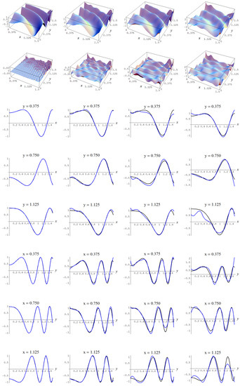
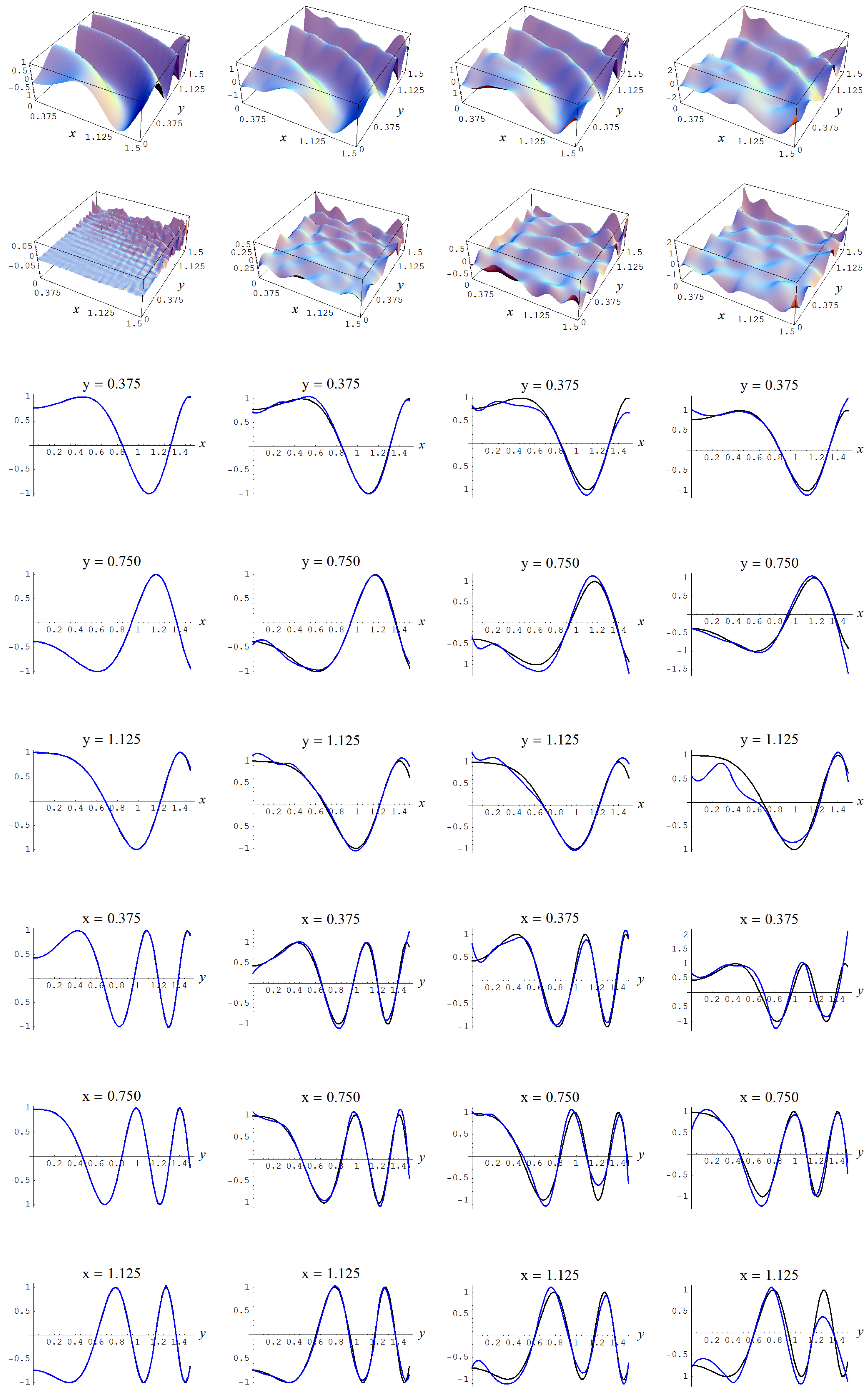
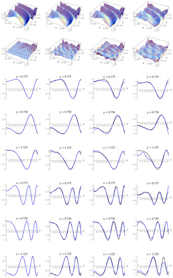
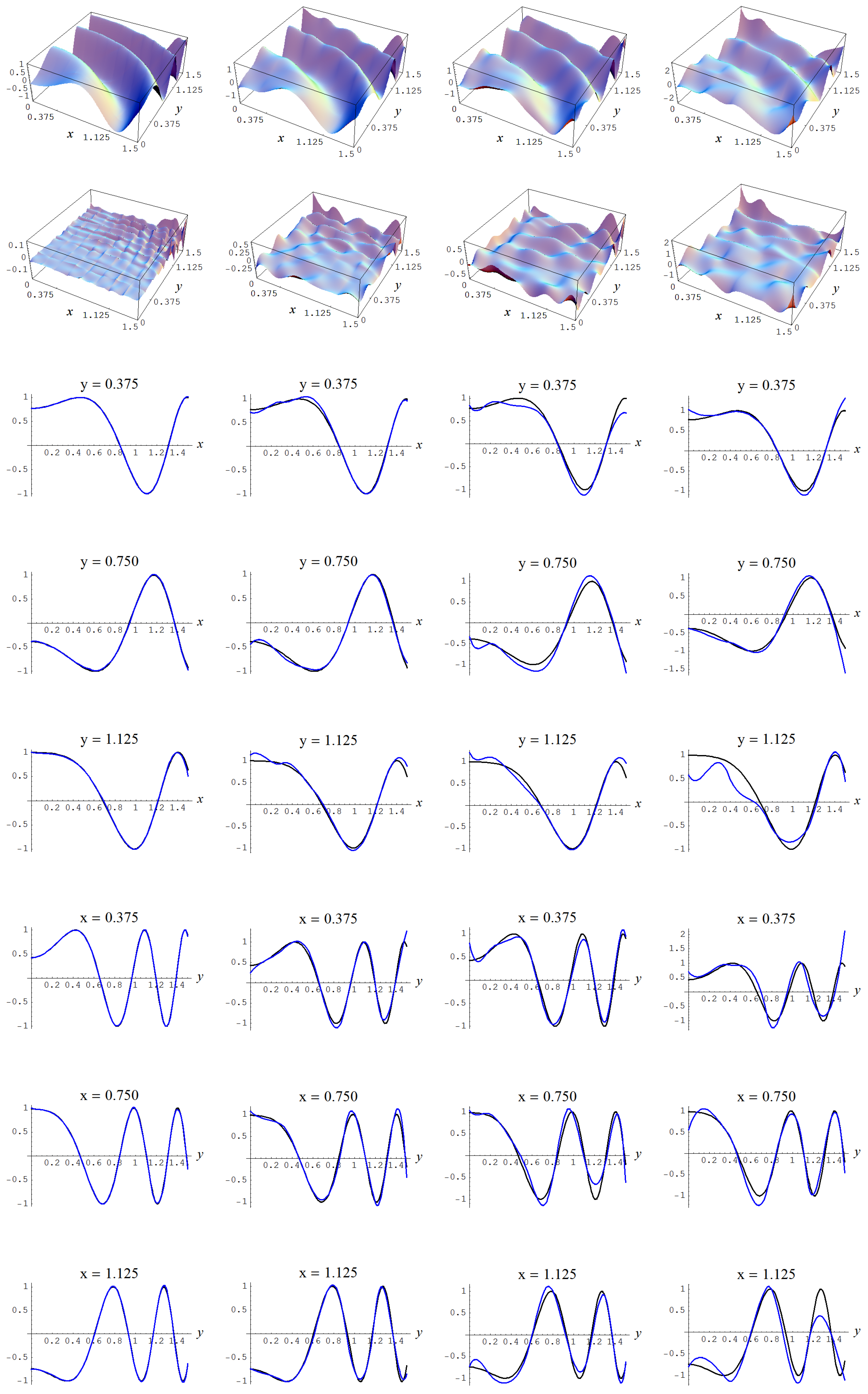
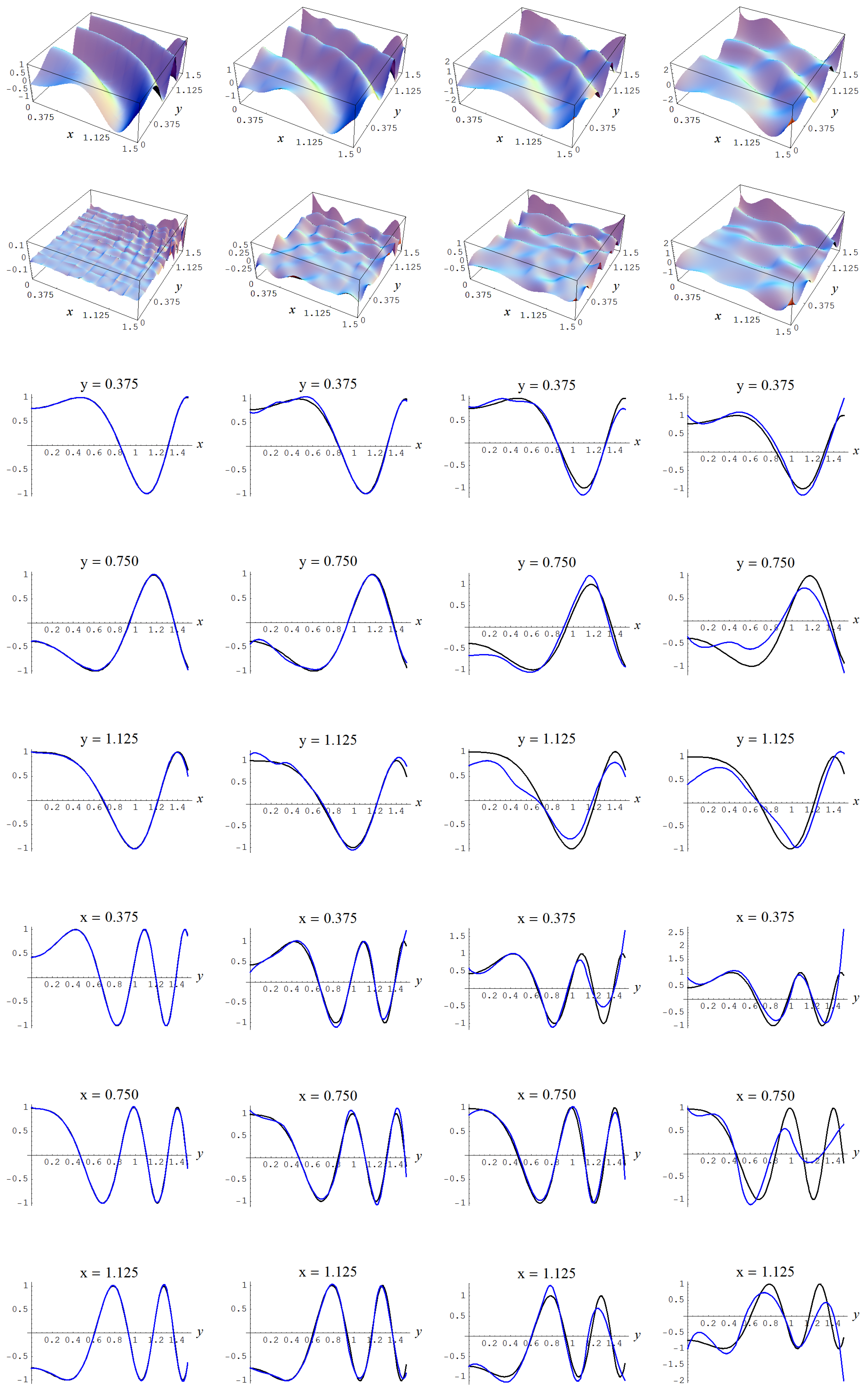
Figure A13.
Sample size N = 15,000 and C-spline models of target function (A7) are picked by the “sure thing” evidence (41) for different noise levels. Columns correspond with noise levels , and 2, respectively. Rows correspond with spline model, residual of spline model relative to target function, and cross sections of spline model (blue) and target function (black).
Figure A14.
Sample size N = 15,000 and C-spline models of target function (A7) are picked by the AIC evidence (143) for different noise levels. Columns correspond with noise levels , and 2, respectively. Rows correspond with spline model, residual of spline model relative to target function, and cross sections of spline model (blue) and target function (black).
Figure A15.
Sample size N = 15,000 and C-spline models of target function (A7) are picked by the Constantineau evidence (130) for different noise levels. Columns correspond with noise levels , and 2, respectively. Rows correspond with spline model, residual of spline model relative to target function, and cross sections of spline model (blue) and target function (black).
Figure A16.
Sample size N = 15,000 and C-spline models of target function (A7) are picked by the Neeley evidence (129) for different noise levels and for a straightforward data estimate of . Columns correspond with noise levels , and 2, respectively. Rows correspond with spline model, residual of spline model relative to target function, and cross sections of spline model (blue) and target function (black).
Figure A17.
Sample size N = 15,000 and C-spline models of target function (A7) are picked by the Ignorance, Manor, and BIC evidences, (135), (127), and (128), for different noise levels and for straightforward data estimates of , , and . Columns correspond with noise levels , and 2, respectively. Rows correspond with spline model, residual of spline model relative to target function, and cross sections of spline model (blue) and target function (black).
It is found, Table A6, that for a multiplication factor of 10 for the data estimates of , , , and , and a Gaussian noise level of the Ignorance and Manor evidences become more conservative than the BIC. Also, for Gaussian noise levels of and the Neely evidence becomes just as conservative as the BIC.
Table A6.
C-spline models (geometry g, polynomial order d, continuity order r) and number of parameters m that were chosen by the discussed evidences, for , under Gaussian noise levels , and 2, and a multiplication factor of 10 for the estimates of the characteristics of the dependent variable y.
Table A6.
C-spline models (geometry g, polynomial order d, continuity order r) and number of parameters m that were chosen by the discussed evidences, for , under Gaussian noise levels , and 2, and a multiplication factor of 10 for the estimates of the characteristics of the dependent variable y.
| Evidences | Model | Model | Model | Model | ||||
|---|---|---|---|---|---|---|---|---|
| “Sure thing” (41) | 1600 | 1600 | 1600 | 1600 | ||||
| AIC (143) | 1600 | 196 | 144 | 121 | ||||
| Constantineau (130) | 1600 | 144 | 121 | 100 | ||||
| Neeley (127) | 625 | 144 | 100 | 64 | ||||
| BIC (135) | 625 | 144 | 100 | 64 | ||||
| Ignorance (127), Manor (127) | 625 | 121 | 100 | 64 | ||||
Data estimates times 10: , , , and ; Data estimates times 10: , , , and ; Data estimates times 10: , , , and ; Data estimates times 10: , , , and .
In Figure A18 and Figure A19, the fitted C-spline models are given for the Neeley evidence and the Ignorance and Manor evidences, respectively. In Figure A19 there is a possible instance of slight under-fitting for a noise level (i.e., column 2) by the model which is picked by the Ignorance and Manor evidences.
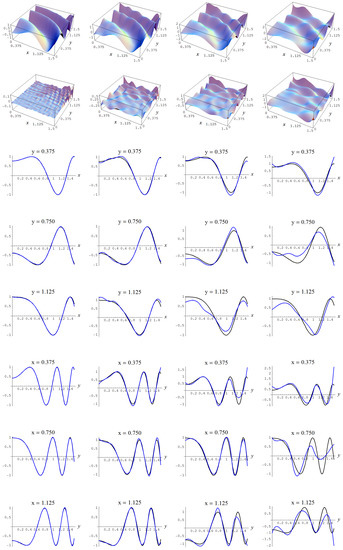

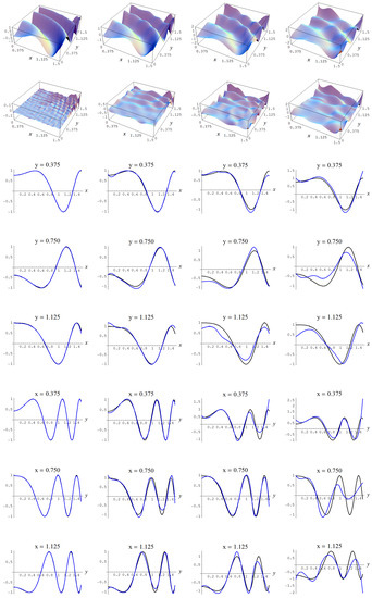
Figure A18.
Sample size and C-spline models of target function (A7) are picked by the Neeley evidence (129), for different noise levels and for a multiplication by a factor 10 of the data estimate of . Columns correspond with noise levels , and 2, respectively. Rows correspond with spline model, residual of spline model relative to target function, and cross sections of spline model (blue) and target function (black).
Figure A19.
Sample size and C-spline models of target function (A7) are picked by the Ignorance and Manorevidences, (127) and (128), for different noise levels and for a multiplication by a factor 10 of , , and . Columns correspond with noise levels , and 2, respectively. Rows correspond with spline model, residual of spline model relative to target function, and cross sections of spline model (blue) and target function (black).
The full outputs of the Bayesian model selection analyses of Table A5 and Table A6 for the Gaussian noise level of are given in Table A7, Table A8, Table A9 and Table A10, respectively.
Table A7.
First half output of the model selection analysis for data sampled from target function (A7), sample size N = 15,000, Gaussian error of , and straightforward data estimates of , , , and ; given are (internally) ranked logarithms of the discussed evidences, ranked sample error standard deviations (from low to high) and R-square values, number of parameters m, and spline model specifications (geometry, polynomial-order, and continuity-order).
| Ignorance | Manor | Neeley | Constantineau | BIC | AIC | “Sure Thing” | Error Std | R-Square | m | Model Specs | |||||||||||
|---|---|---|---|---|---|---|---|---|---|---|---|---|---|---|---|---|---|---|---|---|---|
| 1 | −72,645 | 1 | −72,642 | 3 | −72,511 | 5 | −72,465 | 1 | −72,649 | 23 | −72,268 | 44 | −72,168 | 44 | 1.00 | 44 | 0.32 | 100 | 4 | 3 | 1 |
| 2 | −72,656 | 2 | −72,653 | 1 | −72,493 | 1 | −72,438 | 3 | −72,671 | 7 | −72,210 | 39 | −72,089 | 39 | 1.00 | 39 | 0.33 | 121 | 8 | 3 | 2 |
| 3 | −72,660 | 3 | −72,657 | 2 | −72,498 | 2 | −72,443 | 4 | −72,675 | 9 | −72,215 | 41 | −72,094 | 41 | 1.00 | 41 | 0.33 | 121 | 9 | 2 | 1 |
| 4 | −72,665 | 4 | −72,663 | 7 | −72,532 | 9 | −72,486 | 2 | −72,670 | 27 | −72,289 | 45 | −72,189 | 45 | 1.00 | 45 | 0.32 | 100 | 7 | 3 | 2 |
| 5 | −72,692 | 5 | −72,689 | 6 | −72,530 | 6 | −72,475 | 6 | −72,708 | 20 | −72,247 | 42 | −72,126 | 42 | 1.00 | 42 | 0.32 | 121 | 5 | 2 | 0 |
| 6 | −72,692 | 6 | −72,690 | 10 | −72,558 | 13 | −72,513 | 5 | −72,696 | 30 | −72,316 | 46 | −72,216 | 46 | 1.01 | 46 | 0.32 | 100 | 8 | 2 | 1 |
| 7 | −72,706 | 7 | −72,703 | 4 | −72,513 | 3 | −72,447 | 10 | −72,736 | 1 | −72,188 | 33 | −72,044 | 33 | 1.00 | 33 | 0.33 | 144 | 5 | 3 | 1 |
| 8 | −72,711 | 8 | −72,708 | 5 | −72,518 | 4 | −72,452 | 12 | −72,741 | 3 | −72,193 | 34 | −72,049 | 34 | 1.00 | 34 | 0.33 | 144 | 10 | 2 | 1 |
| 9 | −72,718 | 9 | −72,716 | 9 | −72,556 | 12 | −72,502 | 9 | −72,734 | 24 | −72,273 | 43 | −72,152 | 43 | 1.00 | 43 | 0.32 | 121 | 10 | 1 | 0 |
| 10 | −72,722 | 10 | −72,720 | 19 | −72,613 | 25 | −72,577 | 7 | −72,717 | 37 | −72,409 | 49 | −72,328 | 49 | 1.01 | 49 | 0.31 | 81 | 4 | 2 | 0 |
| 11 | −72,729 | 11 | −72,728 | 21 | −72,621 | 26 | −72,585 | 8 | −72,725 | 38 | −72,417 | 50 | −72,336 | 50 | 1.01 | 50 | 0.31 | 81 | 8 | 1 | 0 |
| 12 | −72,734 | 12 | −72,731 | 15 | −72,600 | 20 | −72,555 | 11 | −72,738 | 32 | −72,357 | 47 | −72,257 | 47 | 1.01 | 47 | 0.31 | 100 | 9 | 1 | 0 |
| 13 | −72,736 | 13 | −72,733 | 8 | −72,543 | 7 | −72,478 | 15 | −72,767 | 11 | −72,218 | 38 | −72,074 | 38 | 1.00 | 38 | 0.33 | 144 | 9 | 3 | 2 |
| 14 | −72,738 | 14 | −72,735 | 17 | −72,604 | 21 | −72,559 | 13 | −72,742 | 33 | −72,362 | 48 | −72,262 | 48 | 1.01 | 48 | 0.31 | 100 | 3 | 3 | 0 |
| 15 | −72,752 | 15 | −72,749 | 11 | −72,559 | 10 | −72,494 | 16 | −72,783 | 14 | −72,234 | 40 | −72,090 | 40 | 1.00 | 40 | 0.33 | 144 | 11 | 1 | 0 |
| 16 | −72,768 | 16 | −72,767 | 25 | −72,660 | 28 | −72,624 | 14 | −72,765 | 40 | −72,456 | 51 | −72,375 | 51 | 1.02 | 51 | 0.30 | 81 | 7 | 2 | 1 |
| 17 | −72,787 | 17 | −72,783 | 12 | −72,561 | 8 | −72,483 | 17 | −72,835 | 2 | −72,192 | 27 | −72,023 | 27 | 0.99 | 27 | 0.33 | 169 | 11 | 2 | 1 |
| 18 | −72,798 | 18 | −72,794 | 13 | −72,572 | 11 | −72,494 | 20 | −72,847 | 5 | −72,203 | 31 | −72,034 | 31 | 0.99 | 31 | 0.33 | 169 | 6 | 2 | 0 |
| 19 | −72,821 | 19 | −72,817 | 14 | −72,594 | 14 | −72,517 | 22 | −72,869 | 13 | −72,226 | 35 | −72,057 | 35 | 1.00 | 35 | 0.33 | 169 | 10 | 3 | 2 |
| 20 | −72,830 | 20 | −72,826 | 16 | −72,603 | 16 | −72,526 | 23 | −72,878 | 15 | −72,234 | 36 | −72,065 | 36 | 1.00 | 36 | 0.33 | 169 | 12 | 1 | 0 |
| 21 | −72,832 | 21 | −72,828 | 18 | −72,605 | 17 | −72,528 | 24 | −72,880 | 17 | −72,237 | 37 | −72,068 | 37 | 1.00 | 37 | 0.33 | 169 | 4 | 3 | 0 |
| 22 | −72,847 | 22 | −72,845 | 29 | −72,739 | 33 | −72,703 | 18 | −72,843 | 44 | −72,535 | 52 | −72,454 | 52 | 1.02 | 52 | 0.29 | 81 | 6 | 3 | 2 |
| 23 | −72,853 | 23 | −72,852 | 32 | −72,768 | 34 | −72,740 | 19 | −72,844 | 46 | −72,600 | 53 | −72,536 | 53 | 1.03 | 53 | 0.29 | 64 | 3 | 3 | 1 |
| 24 | −72,859 | 24 | −72,858 | 33 | −72,774 | 35 | −72,746 | 21 | −72,849 | 47 | −72,606 | 54 | −72,542 | 54 | 1.03 | 54 | 0.29 | 64 | 7 | 1 | 0 |
| 25 | −72,876 | 25 | −72,872 | 20 | −72,613 | 15 | −72,523 | 26 | −72,946 | 4 | −72,200 | 25 | −72,004 | 25 | 0.99 | 25 | 0.34 | 196 | 12 | 2 | 1 |
| 26 | −72,890 | 26 | −72,886 | 22 | −72,628 | 18 | −72,538 | 27 | −72,960 | 8 | −72,214 | 26 | −72,018 | 26 | 0.99 | 26 | 0.33 | 196 | 6 | 3 | 1 |
| 27 | −72,902 | 27 | −72,897 | 23 | −72,639 | 19 | −72,549 | 28 | −72,972 | 12 | −72,225 | 29 | −72,029 | 29 | 0.99 | 29 | 0.33 | 196 | 13 | 1 | 0 |
| 28 | −72,913 | 29 | −72,912 | 36 | −72,828 | 39 | −72,800 | 25 | −72,904 | 49 | −72,660 | 55 | −72,596 | 55 | 1.03 | 55 | 0.28 | 64 | 6 | 2 | 1 |
| 29 | −72,913 | 28 | −72,909 | 24 | −72,650 | 22 | −72,561 | 29 | −72,983 | 18 | −72,237 | 32 | −72,041 | 32 | 0.99 | 32 | 0.33 | 196 | 11 | 3 | 2 |
| 30 | −72,969 | 30 | −72,963 | 26 | −72,667 | 23 | −72,563 | 30 | −73,063 | 6 | −72,207 | 20 | −71,982 | 20 | 0.99 | 20 | 0.34 | 225 | 7 | 2 | 0 |
| 31 | −72,977 | 31 | −72,971 | 27 | −72,675 | 24 | −72,571 | 31 | −73,072 | 10 | −72,215 | 23 | −71,990 | 23 | 0.99 | 23 | 0.34 | 225 | 13 | 2 | 1 |
| 32 | −73,019 | 32 | −73,014 | 28 | −72,717 | 27 | −72,614 | 33 | −73,114 | 22 | −72,257 | 30 | −72,032 | 30 | 0.99 | 30 | 0.33 | 225 | 12 | 3 | 2 |
| 33 | −73,091 | 33 | −73,085 | 30 | −72,747 | 29 | −72,630 | 34 | −73,215 | 19 | −72,240 | 21 | −71,984 | 21 | 0.99 | 21 | 0.34 | 256 | 5 | 3 | 0 |
| 34 | −73,099 | 34 | −73,098 | 40 | −73,014 | 42 | −72,987 | 32 | −73,090 | 53 | −72,847 | 56 | −72,783 | 56 | 1.05 | 56 | 0.26 | 64 | 5 | 3 | 2 |
| 35 | −73,106 | 35 | −73,101 | 31 | −72,763 | 30 | −72,646 | 35 | −73,231 | 21 | −72,256 | 24 | −72,000 | 24 | 0.99 | 24 | 0.34 | 256 | 7 | 3 | 1 |
| 36 | −73,133 | 36 | −73,127 | 34 | −72,790 | 32 | −72,672 | 38 | −73,258 | 25 | −72,283 | 28 | −72,027 | 28 | 0.99 | 28 | 0.33 | 256 | 13 | 3 | 2 |
| 37 | −73,179 | 37 | −73,173 | 35 | −72,791 | 31 | −72,658 | 40 | −73,336 | 16 | −72,235 | 14 | −71,946 | 14 | 0.99 | 14 | 0.34 | 289 | 8 | 2 | 0 |
| 38 | −73,250 | 38 | −73,249 | 43 | −73,185 | 47 | −73,165 | 36 | −73,238 | 55 | −73,051 | 57 | −73,002 | 57 | 1.06 | 57 | 0.24 | 49 | 6 | 1 | 0 |
| 39 | −73,263 | 39 | −73,262 | 44 | −73,198 | 48 | −73,178 | 37 | −73,251 | 56 | −73,064 | 58 | −73,015 | 58 | 1.06 | 58 | 0.24 | 49 | 5 | 2 | 1 |
Table A8.
Second half output of the model selection analysis for data sampled from target function (A7), sample size N = 15,000, Gaussian error of , and straightforward data estimates of , , , and ; given are (internally) ranked logarithms of the discussed evidences, ranked sample error standard deviations (from low to high) and R-square values, number of parameters m, and spline model specifications (geometry, polynomial-order, and continuity-order).
| Ignorance | Manor | Neeley | Constantineau | BIC | AIC | “Sure Thing” | Error Std | R-Square | m | Model Specs | |||||||||||
|---|---|---|---|---|---|---|---|---|---|---|---|---|---|---|---|---|---|---|---|---|---|
| 40 | −73,274 | 40 | −73,273 | 45 | −73,209 | 50 | −73,189 | 39 | −73,262 | 57 | −73,076 | 59 | −73,027 | 59 | 1.06 | 59 | 0.24 | 49 | 3 | 2 | 0 |
| 41 | −73,351 | 41 | −73,344 | 37 | −72,917 | 36 | −72,768 | 43 | −73,546 | 29 | −72,312 | 22 | −71,988 | 22 | 0.99 | 22 | 0.34 | 324 | 8 | 3 | 1 |
| 42 | −73,389 | 42 | −73,387 | 49 | −73,324 | 53 | −73,303 | 41 | −73,377 | 59 | −73,190 | 60 | −73,141 | 60 | 1.07 | 60 | 0.23 | 49 | 2 | 3 | 0 |
| 43 | −73,399 | 43 | −73,398 | 50 | −73,335 | 54 | −73,314 | 42 | −73,388 | 60 | −73,201 | 61 | −73,152 | 61 | 1.07 | 61 | 0.23 | 49 | 4 | 3 | 2 |
| 44 | −73,425 | 44 | −73,416 | 38 | −72,940 | 37 | −72,773 | 44 | −73,659 | 26 | −72,284 | 12 | −71,923 | 12 | 0.99 | 12 | 0.34 | 361 | 9 | 2 | 0 |
| 45 | −73,449 | 45 | −73,440 | 39 | −72,964 | 38 | −72,798 | 45 | −73,684 | 28 | −72,309 | 15 | −71,948 | 15 | 0.99 | 15 | 0.34 | 361 | 6 | 3 | 0 |
| 46 | −73,621 | 46 | −73,612 | 41 | −73,085 | 41 | −72,900 | 47 | −73,902 | 34 | −72,379 | 19 | −71,979 | 19 | 0.99 | 19 | 0.34 | 400 | 9 | 3 | 1 |
| 47 | −73,680 | 47 | −73,670 | 42 | −73,088 | 40 | −72,883 | 52 | −74,009 | 31 | −72,330 | 9 | −71,889 | 9 | 0.98 | 9 | 0.35 | 441 | 10 | 2 | 0 |
| 48 | −73,787 | 48 | −73,786 | 56 | −73,739 | 59 | −73,725 | 46 | −73,774 | 62 | −73,637 | 62 | −73,601 | 62 | 1.10 | 62 | 0.18 | 36 | 5 | 1 | 0 |
| 49 | −73,866 | 49 | −73,855 | 46 | −73,216 | 43 | −72,992 | 56 | −74,250 | 36 | −72,407 | 11 | −71,923 | 11 | 0.99 | 11 | 0.34 | 484 | 7 | 3 | 0 |
| 50 | −73,912 | 50 | −73,901 | 48 | −73,263 | 45 | −73,040 | 57 | −74,298 | 39 | −72,454 | 18 | −71,970 | 18 | 0.99 | 18 | 0.34 | 484 | 10 | 3 | 1 |
| 51 | −73,959 | 52 | −73,958 | 59 | −73,911 | 61 | −73,897 | 48 | −73,946 | 63 | −73,809 | 63 | −73,773 | 63 | 1.12 | 63 | 0.16 | 36 | 2 | 3 | 1 |
| 52 | −73,959 | 53 | −73,958 | 60 | −73,926 | 62 | −73,916 | 49 | −73,946 | 64 | −73,851 | 65 | −73,826 | 65 | 1.12 | 65 | 0.15 | 25 | 2 | 2 | 0 |
| 53 | −73,967 | 51 | −73,955 | 47 | −73,257 | 44 | −73,011 | 58 | −74,409 | 35 | −72,394 | 7 | −71,865 | 7 | 0.98 | 7 | 0.35 | 529 | 11 | 2 | 0 |
| 54 | −73,980 | 54 | −73,980 | 61 | −73,947 | 63 | −73,938 | 50 | −73,968 | 66 | −73,872 | 66 | −73,847 | 66 | 1.12 | 66 | 0.15 | 25 | 4 | 1 | 0 |
| 55 | −74,001 | 55 | −74,000 | 62 | −73,954 | 64 | −73,940 | 51 | −73,989 | 65 | −73,852 | 64 | −73,816 | 64 | 1.12 | 64 | 0.15 | 36 | 4 | 2 | 1 |
| 56 | −74,105 | 56 | −74,105 | 63 | −74,058 | 65 | −74,044 | 53 | −74,093 | 67 | −73,956 | 67 | −73,920 | 67 | 1.13 | 67 | 0.14 | 36 | 3 | 3 | 2 |
| 57 | −74,193 | 57 | −74,192 | 65 | −74,160 | 67 | −74,151 | 54 | −74,180 | 68 | −74,085 | 68 | −74,060 | 68 | 1.14 | 68 | 0.13 | 25 | 3 | 2 | 1 |
| 58 | −74,221 | 58 | −74,208 | 52 | −73,448 | 49 | −73,183 | 64 | −74,729 | 45 | −72,536 | 17 | −71,960 | 17 | 0.99 | 17 | 0.34 | 576 | 11 | 3 | 1 |
| 59 | −74,247 | 59 | −74,247 | 66 | −74,215 | 68 | −74,205 | 55 | −74,235 | 69 | −74,140 | 69 | −74,115 | 69 | 1.14 | 69 | 0.12 | 25 | 2 | 3 | 2 |
| 60 | −74,279 | 60 | −74,265 | 51 | −73,440 | 46 | −73,149 | 68 | −74,852 | 41 | −72,472 | 6 | −718,47 | 6 | 0.98 | 6 | 0.35 | 625 | 12 | 2 | 0 |
| 61 | −74,320 | 61 | −74,306 | 53 | −73,481 | 51 | −73,191 | 69 | −74,894 | 42 | −72,514 | 10 | −71,889 | 10 | 0.98 | 10 | 0.35 | 625 | 8 | 3 | 0 |
| 62 | −74,430 | 62 | −74,430 | 67 | −74,410 | 70 | −74,404 | 59 | −74,420 | 70 | −74,359 | 70 | −74,343 | 70 | 1.16 | 70 | 0.09 | 16 | 2 | 2 | 1 |
| 63 | −74,462 | 65 | −74,462 | 71 | −74,441 | 73 | −74,435 | 62 | −74,452 | 73 | −74,391 | 73 | −74,375 | 71 | 1.16 | 73 | 0.09 | 16 | 1 | 3 | 0 |
| 64 | −74,462 | 64 | −74,462 | 70 | −74,441 | 72 | −74,435 | 61 | −74,452 | 72 | −74,391 | 72 | −74,375 | 72 | 1.16 | 72 | 0.09 | 16 | 1 | 3 | 1 |
| 65 | −74,462 | 63 | −74,462 | 69 | −74,441 | 71 | −74,435 | 60 | −74,452 | 71 | −74,391 | 71 | −74,375 | 73 | 1.16 | 71 | 0.09 | 16 | 1 | 3 | 2 |
| 66 | −74,476 | 66 | −74,475 | 72 | −74,455 | 74 | −74,449 | 63 | −74,465 | 74 | −74,404 | 74 | −74,388 | 74 | 1.16 | 74 | 0.09 | 16 | 3 | 1 | 0 |
| 67 | −74,551 | 67 | −74,535 | 55 | −73,644 | 55 | −73,332 | 71 | −75,200 | 48 | −72,626 | 16 | −71,950 | 16 | 0.99 | 16 | 0.34 | 676 | 12 | 3 | 1 |
| 68 | −74,578 | 68 | −74,561 | 54 | −73,598 | 52 | −73,257 | 72 | −75,299 | 43 | −72,523 | 3 | −71,794 | 3 | 0.98 | 3 | 0.35 | 729 | 13 | 2 | 0 |
| 69 | −74,781 | 69 | −74,781 | 74 | −74,770 | 75 | −74,766 | 65 | −74,773 | 75 | −74,739 | 75 | −74,730 | 75 | 1.19 | 75 | 0.04 | 9 | 2 | 1 | 0 |
| 70 | −74,845 | 72 | −74,845 | 76 | −74,834 | 77 | −74,830 | 67 | −74,837 | 77 | −74,803 | 77 | −74,794 | 76 | 1.20 | 77 | 0.04 | 9 | 1 | 2 | 0 |
| 71 | −74,845 | 71 | −74,845 | 75 | −74,834 | 76 | −74,830 | 66 | −74,837 | 76 | −74,803 | 76 | −74,794 | 77 | 1.20 | 76 | 0.04 | 9 | 1 | 2 | 1 |
| 72 | −74,849 | 70 | −74,831 | 57 | −73,796 | 56 | −73,433 | 73 | −75,657 | 50 | −72,672 | 8 | −71,888 | 8 | 0.98 | 8 | 0.35 | 784 | 9 | 3 | 0 |
| 73 | −74,903 | 73 | −74,885 | 58 | −73,851 | 57 | −73,489 | 74 | −75,714 | 51 | −72,728 | 13 | −71,944 | 13 | 0.99 | 13 | 0.34 | 784 | 13 | 3 | 1 |
| 74 | −74,932 | 74 | −74,932 | 77 | −74,927 | 78 | −74,926 | 70 | −74,928 | 78 | −74,913 | 78 | −74,909 | 78 | 1.20 | 78 | 0.02 | 4 | 1 | 1 | 0 |
| 75 | −75,377 | 75 | −75,355 | 64 | −74,086 | 58 | −73,638 | 75 | −76,462 | 52 | −72,802 | 5 | −71,841 | 5 | 0.98 | 5 | 0.35 | 961 | 10 | 3 | 0 |
| 76 | −75,965 | 76 | −75,938 | 68 | −74,412 | 60 | −73,872 | 76 | −77,375 | 54 | −72,973 | 4 | −71,817 | 4 | 0.98 | 4 | 0.35 | 1156 | 11 | 3 | 0 |
| 77 | −76,591 | 77 | −76,560 | 73 | −74,751 | 66 | −74,111 | 77 | −78,374 | 58 | −73,161 | 2 | −71,792 | 2 | 0.98 | 2 | 0.35 | 1369 | 12 | 3 | 0 |
| 78 | −77,238 | 78 | −77,201 | 78 | −75,086 | 69 | −74,335 | 78 | −79,441 | 61 | −73,349 | 1 | −71,749 | 1 | 0.98 | 1 | 0.36 | 1600 | 13 | 3 | 0 |
Table A9.
First half output of the model selection analysis for data sampled from target function (A7), sample size N = 15,000, Gaussian error of , and times 10 data estimates of , , , and ; given are (internally) ranked logarithms of the discussed evidences, ranked sample error standard deviations (from low to high) and R-square values, number of parameters m, and spline model specifications (geometry, polynomial-order, and continuity-order).
| Ignorance | Manor | Neeley | Constantineau | BIC | AIC | “Sure Thing” | Error Std | R-Square | m | Model Specs | |||||||||||
|---|---|---|---|---|---|---|---|---|---|---|---|---|---|---|---|---|---|---|---|---|---|
| 1 | −72,859 | 1 | −72,856 | 1 | −72,715 | 5 | −72,465 | 1 | −72,649 | 23 | −72,268 | 44 | −72,168 | 44 | 1.00 | 44 | 0.32 | 100 | 4 | 3 | 1 |
| 2 | −72,879 | 2 | −72,877 | 2 | −72,736 | 9 | −72,486 | 2 | −72,670 | 27 | −72,289 | 45 | −72,189 | 45 | 1.00 | 45 | 0.32 | 100 | 7 | 3 | 2 |
| 3 | −72,895 | 3 | −72,893 | 7 | −72,779 | 25 | −72,577 | 7 | −72,717 | 37 | −72,409 | 49 | −72,328 | 49 | 1.01 | 49 | 0.31 | 81 | 4 | 2 | 0 |
| 4 | −72,903 | 4 | −72,900 | 8 | −72,787 | 26 | −72,585 | 8 | −72,725 | 38 | −72,417 | 50 | −72,336 | 50 | 1.01 | 50 | 0.31 | 81 | 8 | 1 | 0 |
| 5 | −72,906 | 5 | −72,903 | 5 | −72,763 | 13 | −72,513 | 5 | −72,696 | 30 | −72,316 | 46 | −72,216 | 46 | 1.01 | 46 | 0.32 | 100 | 8 | 2 | 1 |
| 6 | −72,915 | 6 | −72,911 | 3 | −72,741 | 1 | −72,438 | 3 | −72,671 | 7 | −72,210 | 39 | −72,089 | 39 | 1.00 | 39 | 0.33 | 121 | 8 | 3 | 2 |
| 7 | −72,919 | 7 | −72,916 | 4 | −72,746 | 2 | −72,443 | 4 | −72,675 | 9 | −72,215 | 41 | −72,094 | 41 | 1.00 | 41 | 0.33 | 121 | 9 | 2 | 1 |
| 8 | −72,942 | 8 | −72,939 | 14 | −72,826 | 28 | −72,624 | 14 | −72,765 | 40 | −72,456 | 51 | −-72,375 | 51 | 1.02 | 51 | 0.30 | 81 | 7 | 2 | 1 |
| 9 | −72,948 | 9 | −72,945 | 10 | −72,804 | 20 | −72,555 | 11 | −72,738 | 32 | −72,357 | 47 | −72,257 | 47 | 1.01 | 47 | 0.31 | 100 | 9 | 1 | 0 |
| 10 | −72,951 | 10 | −72,948 | 6 | −72,778 | 6 | −72,475 | 6 | −72,708 | 20 | −72,247 | 42 | −72,126 | 42 | 1.00 | 42 | 0.32 | 121 | 5 | 2 | 0 |
| 11 | −72,952 | 11 | −72,949 | 11 | −72,809 | 21 | −72,559 | 13 | −72,742 | 33 | −72,362 | 48 | −72,262 | 48 | 1.01 | 48 | 0.31 | 100 | 3 | 3 | 0 |
| 12 | −72,977 | 12 | −72,974 | 9 | −72,804 | 12 | −72,502 | 9 | −72,734 | 24 | −72,273 | 43 | −72,152 | 43 | 1.00 | 43 | 0.32 | 121 | 10 | 1 | 0 |
| 13 | −72,990 | 13 | −72,988 | 17 | −72,898 | 34 | −72,740 | 19 | −72,844 | 46 | −72,600 | 53 | −72,536 | 53 | 1.03 | 53 | 0.29 | 64 | 3 | 3 | 1 |
| 14 | −72,996 | 14 | −72,994 | 19 | −72,904 | 35 | −72,746 | 21 | −72,849 | 47 | −72,606 | 54 | −72,542 | 54 | 1.03 | 54 | 0.29 | 64 | 7 | 1 | 0 |
| 15 | −73,015 | 15 | −73,011 | 12 | −72,809 | 3 | −72,447 | 10 | −72,736 | 1 | −72,188 | 33 | −72,044 | 33 | 1.00 | 33 | 0.33 | 144 | 5 | 3 | 1 |
| 16 | −73,019 | 16 | −73,015 | 13 | −72,813 | 4 | −72,452 | 12 | −72,741 | 3 | −72,193 | 34 | −72,049 | 34 | 1.00 | 34 | 0.33 | 144 | 10 | 2 | 1 |
| 17 | −73,020 | 17 | −73,018 | 18 | −72,904 | 33 | −72,703 | 18 | −72,843 | 44 | −72,535 | 52 | −72,454 | 52 | 1.02 | 52 | 0.29 | 81 | 6 | 3 | 2 |
| 18 | −73,045 | 18 | −73,041 | 15 | −72,839 | 7 | −72,478 | 15 | −72,767 | 11 | −72,218 | 38 | −72,074 | 38 | 1.00 | 38 | 0.33 | 144 | 9 | 3 | 2 |
| 19 | −73,050 | 19 | −73,048 | 25 | −72,958 | 39 | −72,800 | 25 | −72,904 | 49 | −72,660 | 55 | −72,596 | 55 | 1.03 | 55 | 0.28 | 64 | 6 | 2 | 1 |
| 20 | −73,060 | 20 | −73,057 | 16 | −72,854 | 10 | −72,494 | 16 | −72,783 | 14 | −72,234 | 40 | −72,090 | 40 | 1.00 | 40 | 0.33 | 144 | 11 | 1 | 0 |
| 21 | −73,149 | 21 | −73,145 | 20 | −72,907 | 8 | −72,483 | 17 | −72,835 | 2 | −72,192 | 27 | −72,023 | 27 | 0.99 | 27 | 0.33 | 169 | 11 | 2 | 1 |
| 22 | −73,160 | 22 | −73,156 | 21 | −72,918 | 11 | −72,494 | 20 | −72,847 | 5 | −72,203 | 31 | −72,034 | 31 | 0.99 | 31 | 0.33 | 169 | 6 | 2 | 0 |
| 23 | −73,183 | 23 | −73,178 | 22 | −72,941 | 14 | −72,517 | 22 | −72,869 | 13 | −72,226 | 35 | −72,057 | 35 | 1.00 | 35 | 0.33 | 169 | 10 | 3 | 2 |
| 24 | −73,191 | 24 | −73,187 | 23 | −72,949 | 16 | −72,526 | 23 | −72,878 | 15 | −72,234 | 36 | −72,065 | 36 | 1.00 | 36 | 0.33 | 169 | 12 | 1 | 0 |
| 25 | −73,193 | 25 | −73,189 | 24 | −72,951 | 17 | −72,528 | 24 | −72,880 | 17 | −72,237 | 37 | −72,068 | 37 | 1.00 | 37 | 0.33 | 169 | 4 | 3 | 0 |
| 26 | −73,236 | 26 | −73,234 | 32 | −73,144 | 42 | −72,987 | 32 | −73,090 | 53 | −72,847 | 56 | −72,783 | 56 | 1.05 | 56 | 0.26 | 64 | 5 | 3 | 2 |
| 27 | −73,296 | 27 | −73,291 | 26 | −73,016 | 15 | −72,523 | 26 | −72,946 | 4 | −72,200 | 25 | −72,004 | 25 | 0.99 | 25 | 0.34 | 196 | 12 | 2 | 1 |
| 28 | −73,310 | 28 | −73,305 | 27 | −73,030 | 18 | −72,538 | 27 | −72,960 | 8 | −72,214 | 26 | −72,018 | 26 | 0.99 | 26 | 0.33 | 196 | 6 | 3 | 1 |
| 29 | −73,322 | 29 | −73,316 | 28 | −73,041 | 19 | −72,549 | 28 | −72,972 | 12 | −72,225 | 29 | −72,029 | 29 | 0.99 | 29 | 0.33 | 196 | 13 | 1 | 0 |
| 30 | −73,333 | 30 | −73,328 | 29 | −73,052 | 22 | −72,561 | 29 | −72,983 | 18 | −72,237 | 32 | −72,041 | 32 | 0.99 | 32 | 0.33 | 196 | 11 | 3 | 2 |
| 31 | −73,354 | 31 | −73,353 | 35 | −73,284 | 47 | −73,165 | 36 | −73,238 | 55 | −73,051 | 57 | −73,002 | 57 | 1.06 | 57 | 0.24 | 49 | 6 | 1 | 0 |
| 32 | −73,367 | 32 | −73,366 | 37 | −73,297 | 48 | −73,178 | 37 | −73,251 | 56 | −73,064 | 58 | −73,015 | 58 | 1.06 | 58 | 0.24 | 49 | 5 | 2 | 1 |
| 33 | −73,379 | 33 | −73,377 | 38 | −73,308 | 50 | −73,189 | 39 | −73,262 | 57 | −73,076 | 59 | −73,027 | 59 | 1.06 | 59 | 0.24 | 49 | 3 | 2 | 0 |
| 34 | −73,450 | 34 | −73,444 | 30 | −73,128 | 23 | −72,563 | 30 | −73,063 | 6 | −72,207 | 20 | −71,982 | 20 | 0.99 | 20 | 0.34 | 225 | 7 | 2 | 0 |
| 35 | −73,459 | 35 | −73,452 | 31 | −73,137 | 24 | −72,571 | 31 | −73,072 | 10 | −72,215 | 23 | −71,990 | 23 | 0.99 | 23 | 0.34 | 225 | 13 | 2 | 1 |
| 36 | −73,493 | 36 | −73,492 | 41 | −73,423 | 53 | −73,303 | 41 | −73,377 | 59 | −73,190 | 60 | −73,141 | 60 | 1.07 | 60 | 0.23 | 49 | 2 | 3 | 0 |
| 37 | −73,501 | 37 | −73,495 | 33 | −73,179 | 27 | −72,614 | 33 | −73,114 | 22 | −72,257 | 30 | −72,032 | 30 | 0.99 | 30 | 0.33 | 225 | 12 | 3 | 2 |
| 38 | −73,504 | 38 | −73,502 | 42 | −73,433 | 54 | −73,314 | 42 | −73,388 | 60 | −73,201 | 61 | −73,152 | 61 | 1.07 | 61 | 0.23 | 49 | 4 | 3 | 2 |
| 39 | −73,639 | 39 | −73,632 | 34 | −73,273 | 29 | −72,630 | 34 | −73,215 | 19 | −72,240 | 21 | −71,984 | 21 | 0.99 | 21 | 0.34 | 256 | 5 | 3 | 0 |
Table A10.
Second half output of the model selection analysis for data sampled from target function (A7), sample size N = 15,000, Gaussian error of , and times 10 data estimates of , , , and ; given are (internally) ranked logarithms of the discussed evidences, ranked sample error standard deviations (from low to high) and R-square values, number of parameters m, and spline model specifications (geometry, polynomial-order, and continuity-order).
| Ignorance | Manor | Neeley | Constantineau | BIC | AIC | “Sure Thing” | Error Std | R-Square | m | Model Specs | |||||||||||
|---|---|---|---|---|---|---|---|---|---|---|---|---|---|---|---|---|---|---|---|---|---|
| 40 | −73,655 | 40 | −73,648 | 36 | −73,288 | 30 | −72,646 | 35 | −73,231 | 21 | −72,256 | 24 | −72,000 | 24 | 0.99 | 24 | 0.34 | 256 | 7 | 3 | 1 |
| 41 | −73,681 | 41 | −73,674 | 39 | −73,315 | 32 | −72,672 | 38 | −73,258 | 25 | −72,283 | 28 | −72,027 | 28 | 0.99 | 28 | 0.33 | 256 | 13 | 3 | 2 |
| 42 | −73,798 | 42 | −73,790 | 40 | -73,385 | 31 | −72,658 | 40 | −73,336 | 16 | −72,235 | 14 | −71,946 | 14 | 0.99 | 14 | 0.34 | 289 | 8 | 2 | 0 |
| 43 | −73,863 | 43 | −73,862 | 46 | −73,811 | 59 | −73,725 | 46 | −73,774 | 62 | −73,637 | 62 | −73,601 | 62 | 1.10 | 62 | 0.18 | 36 | 5 | 1 | 0 |
| 44 | −74,012 | 44 | −74,011 | 48 | −73,976 | 62 | −73,916 | 49 | −73,946 | 64 | −73,851 | 64 | −73,826 | 64 | 1.12 | 64 | 0.15 | 25 | 2 | 2 | 0 |
| 45 | −74,033 | 45 | −74,033 | 51 | −73,997 | 63 | −73,938 | 50 | −73,968 | 65 | −73,872 | 65 | −73,847 | 65 | 1.12 | 65 | 0.15 | 25 | 4 | 1 | 0 |
| 46 | −74,035 | 46 | −74,034 | 49 | −73,983 | 61 | −73,897 | 48 | −73,946 | 63 | −73,809 | 63 | −73,773 | 63 | 1.12 | 63 | 0.16 | 36 | 2 | 3 | 1 |
| 47 | −74,045 | 47 | −74,036 | 43 | −73,582 | 36 | −72,768 | 43 | −73,546 | 29 | −72,312 | 22 | −71,988 | 22 | 0.99 | 22 | 0.34 | 324 | 8 | 3 | 1 |
| 48 | −74,154 | 48 | −74,153 | 52 | −74,103 | 64 | −74,017 | 52 | −74,066 | 66 | −73,929 | 66 | −73,893 | 66 | 1.13 | 66 | 0.15 | 36 | 4 | 2 | 1 |
| 49 | −74,198 | 49 | −74,188 | 44 | −73,681 | 37 | −72,773 | 44 | −73,659 | 26 | −72,284 | 12 | −71,923 | 12 | 0.99 | 12 | 0.34 | 361 | 9 | 2 | 0 |
| 50 | −74,222 | 50 | −74,212 | 45 | −73,705 | 38 | −72,798 | 45 | −73,684 | 28 | −72,309 | 15 | −71,948 | 15 | 0.99 | 15 | 0.34 | 361 | 6 | 3 | 0 |
| 51 | −74,246 | 51 | −74,245 | 54 | −74,210 | 67 | −74,151 | 54 | −74,180 | 68 | −74,085 | 68 | −74,060 | 68 | 1.14 | 68 | 0.13 | 25 | 3 | 2 | 1 |
| 52 | −74,257 | 52 | −74,256 | 53 | −74,206 | 66 | −74,120 | 53 | −74,169 | 67 | −74,032 | 67 | −73,996 | 67 | 1.13 | 67 | 0.13 | 36 | 3 | 3 | 2 |
| 53 | −74,300 | 53 | −74,299 | 57 | −74,264 | 68 | −74,205 | 55 | −74,235 | 69 | −74,140 | 69 | −74,115 | 69 | 1.14 | 69 | 0.12 | 25 | 2 | 3 | 2 |
| 54 | −74,464 | 54 | −74,464 | 59 | −74,441 | 70 | −74,404 | 59 | −74,420 | 70 | −74,359 | 70 | −74,343 | 70 | 1.16 | 70 | 0.09 | 16 | 2 | 2 | 1 |
| 55 | −74,478 | 55 | −74,467 | 47 | −73,905 | 41 | −72,900 | 47 | −73,902 | 34 | −72,379 | 19 | −71,979 | 19 | 0.99 | 19 | 0.34 | 400 | 9 | 3 | 1 |
| 56 | −74,496 | 58 | −74,496 | 62 | −74,473 | 73 | −74,435 | 62 | −74,452 | 73 | −74,391 | 73 | −74,375 | 71 | 1.16 | 73 | 0.09 | 16 | 1 | 3 | 0 |
| 57 | −74,496 | 57 | −74,496 | 61 | −74,473 | 72 | −74,435 | 61 | −74,452 | 72 | −74,391 | 72 | −74,375 | 72 | 1.16 | 72 | 0.09 | 16 | 1 | 3 | 1 |
| 58 | −74,496 | 56 | −74,496 | 60 | −74,473 | 71 | −74,435 | 60 | −74,452 | 71 | −74,391 | 71 | −74,375 | 73 | 1.16 | 71 | 0.09 | 16 | 1 | 3 | 2 |
| 59 | −74,509 | 59 | −74,509 | 63 | −74,487 | 74 | −74,449 | 63 | −74,465 | 74 | −74,404 | 74 | −74,388 | 74 | 1.16 | 74 | 0.09 | 16 | 3 | 1 | 0 |
| 60 | −74,625 | 60 | −74,613 | 50 | −73,994 | 40 | −72,883 | 51 | −74,009 | 31 | −72,330 | 9 | −71,889 | 9 | 0.98 | 9 | 0.35 | 441 | 10 | 2 | 0 |
| 61 | −74,800 | 61 | −74,800 | 67 | −74,787 | 75 | −74,766 | 65 | −74,773 | 75 | −74,739 | 75 | −74,730 | 75 | 1.19 | 75 | 0.04 | 9 | 2 | 1 | 0 |
| 62 | −74,864 | 63 | −74,864 | 69 | −74,851 | 77 | −74,830 | 67 | −74,837 | 77 | −74,803 | 77 | −74,794 | 76 | 1.20 | 77 | 0.04 | 9 | 1 | 2 | 0 |
| 63 | −74,864 | 62 | −74,864 | 68 | −74,851 | 76 | −74,830 | 66 | −74,837 | 76 | −74,803 | 76 | −74,794 | 77 | 1.20 | 76 | 0.04 | 9 | 1 | 2 | 1 |
| 64 | −74,903 | 64 | −74,890 | 55 | −74,210 | 43 | −72,992 | 56 | −74,250 | 36 | −72,407 | 11 | −71,923 | 11 | 0.99 | 11 | 0.34 | 484 | 7 | 3 | 0 |
| 65 | −74,941 | 66 | −74,941 | 70 | −74,935 | 78 | −74,926 | 70 | −74,928 | 78 | −74,913 | 78 | −74,909 | 78 | 1.20 | 78 | 0.02 | 4 | 1 | 1 | 0 |
| 66 | −74,949 | 65 | −74,935 | 56 | −74,256 | 45 | −73,040 | 57 | −74,298 | 39 | −72,454 | 18 | −71,970 | 18 | 0.99 | 18 | 0.34 | 484 | 10 | 3 | 1 |
| 67 | −75,101 | 67 | −75,086 | 58 | −74,344 | 44 | −73,011 | 58 | −74,409 | 35 | −72,394 | 7 | −71,865 | 7 | 0.98 | 7 | 0.35 | 529 | 11 | 2 | 0 |
| 68 | −75,455 | 68 | −75,439 | 64 | −74,630 | 49 | −73,183 | 64 | −74,729 | 45 | −72,536 | 17 | −71,960 | 17 | 0.99 | 17 | 0.34 | 576 | 11 | 3 | 1 |
| 69 | −75,619 | 69 | −75,602 | 65 | −74,724 | 46 | −73,149 | 68 | −74,852 | 41 | −72,472 | 6 | −71,847 | 6 | 0.98 | 6 | 0.35 | 625 | 12 | 2 | 0 |
| 70 | −75,659 | 70 | −75,642 | 66 | −74,765 | 51 | −73,191 | 69 | −74,894 | 42 | −72,514 | 10 | −71,889 | 10 | 0.98 | 10 | 0.35 | 625 | 8 | 3 | 0 |
| 71 | −75,999 | 71 | −75,980 | 71 | −75,031 | 55 | −73,332 | 71 | −75,200 | 48 | −72,626 | 16 | −71,950 | 16 | 0.99 | 16 | 0.34 | 676 | 12 | 3 | 1 |
| 72 | −76,141 | 72 | −76,121 | 72 | −75,097 | 52 | −73,257 | 72 | −75,299 | 43 | −72,523 | 3 | −71,794 | 3 | 0.98 | 3 | 0.35 | 729 | 13 | 2 | 0 |
| 73 | −76,529 | 73 | −76,508 | 73 | −75,407 | 56 | −73,433 | 73 | −75,657 | 50 | −72,672 | 8 | −71,888 | 8 | 0.98 | 8 | 0.35 | 784 | 9 | 3 | 0 |
| 74 | −76,583 | 74 | −76,561 | 74 | −75,461 | 57 | −73,489 | 74 | −75,714 | 51 | −72,728 | 13 | −71,944 | 13 | 0.99 | 13 | 0.34 | 784 | 13 | 3 | 1 |
| 75 | −77,436 | 75 | −77,410 | 75 | −76,061 | 58 | −73,638 | 75 | −76,462 | 52 | −72,802 | 5 | −71,841 | 5 | 0.98 | 5 | 0.35 | 961 | 10 | 3 | 0 |
| 76 | −78,443 | 76 | −78,412 | 76 | −76,789 | 60 | −73,872 | 76 | −77,375 | 54 | −72,973 | 4 | −71,817 | 4 | 0.98 | 4 | 0.35 | 1156 | 11 | 3 | 0 |
| 77 | −79,526 | 77 | −79,489 | 77 | −77,567 | 65 | −74,111 | 77 | −78,374 | 58 | −73,161 | 2 | −71,792 | 2 | 0.98 | 2 | 0.35 | 1369 | 12 | 3 | 0 |
| 78 | −80,668 | 78 | −80,625 | 78 | −78,379 | 69 | −74,335 | 78 | −79,441 | 61 | −73,349 | 1 | −71,749 | 1 | 0.98 | 1 | 0.36 | 1600 | 13 | 3 | 0 |
Appendix B. Introducing C-Splines
Appendix B.1. A Simple Trivariate C-Spline Model
If we have predictors from a three dimensional domain , where , and a corresponding dependent variable v, then the simplest non-trivial spline model is the model which partitions the cube of the three dimensional domain in sub-cubes, has polynomial order 1 with no interactions, that is,
and continuity of order 0 (i.e., piecewise polynomials themselves need to connect, but not their derivatives.) It is found that this particular spline model corresponds with the C-spline basis [5]:
where each of the rows u correspond with a particular sub-domain in .
Let and k be the x-, y-, and z-axis sub-domain coordinates, respectively. Then we have that the row number u of is the following function of the sub-domain coordinates
where the coordinates for a given sub-domain can be found as
Now, if we have a data set with sample size N, then we may go iteratively through this data set, as we determine for each entry in the predictor matrix the corresponding coordinates , by way of (A11):
These coordinates then map to the row , by way of (A10):
We then substitute the values into the vector , which gives us . Finally, we set the nth row of the spline predictor matrix to
As we follow this procedure for , we end up with a spline predictor matrix . If we regress this spline predictor matrix on the dependent variable vector , we obtain the spline regression coefficients
If we combine the functions (A10) and (A11), so as to obtain the sub-domain number directly as a function of x, y, and z,
then the C-spline model on the domain for the expected value (156), with a 2-by-2-by-2 geometry, a polynomial order 1 with no interactions, and continuity order 0 may be written down as the inner product, (A9) and (A12),
In Figure A20 we give a demonstration of the spline equivalent (A14) of the polynomial (A8), by way of the spline basis (A9), where we (arbitrarily and as a reference for the reader) let
Figure A20.
Example of the trivariate C-spline model for (A8), for , , and , respectively.
Figure A20.
Example of the trivariate C-spline model for (A8), for , , and , respectively.
Note that 8 trivariate piecewise polynomials of order 1 with no interactions ordinarily would make for parameters, whereas just the one trivariate piecewise polynomial (A8) over the total unpartitioned domain makes for parameters. Seeing that (A9) consists of parameters, it follows that the constraint for connectedness of the polynomials has incurred a cost of
free parameters relative to the unconstrained case, or, alternatively, a gain of
free parameters relative to the case where one polynomial is defined over the whole of the domain.
Appendix B.2. Enforcing Connectivity
The sub-domains
connect at . The sub-domains and are associated with the sub-domain numbers and , respectively, (A13). It follows that and have corresponding C-spline basis vectors (A9)
and
If we approach the z-boundary of the 4th and the 8th sub-domain, or, equivalent, if we let in the domains and , from below and above, respectively, then it may be checked that the above C-spline basis vectors converge to the same vector:
and
It follows that the C-spline model (A14) will connect at the z-boundary of the sub-domains and , for any regression coefficient vector , as the z-boundary is crossed from below and the inner product goes from
to
and vise versa. It may be checked that this holds for all possible boundary crossings in the domain . Stated differently, the C-spline model (A14) enforces the piecewise polynomials to connect at their domain boundaries by way of its C-spline basis (A9).
Appendix B.3. Adding Polynomial Interaction and Power Terms
Now, the C-spline model (A14) enforces the piecewise polynomials to connect at their domain boundaries by way of its C-spline basis (A9). So, it follows that any product of the columns in (A9) must also enforce this connectedness; to be more specific, if we want to introduce an interaction between x and y, then we just need to multiply the two x-columns with the two y-columns of (A9) in the following manner:
or, equivalently, as any linear combination of columns also will adhere to the constraint of connectivity,
And it may be checked that the addition of these columns to the spline basis (A9) will still result in an enforcement of the constraint of connectedness. (Similarly, one may also row reduce the spline basis (A9), should one wish to do so.)
By way of induction, it follows that the number of columns in the introduction of the spline polynomials interactions , , , and to (A8),
will result in a spline basis which has
free parameters. In Figure A21 we give a demonstration of the added flexibility of the spline equivalent (A14) of the polynomial (A16) for a random .
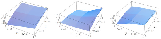

Figure A21.
Example of the trivariate C-spline model for (A16), for , , and , respectively.
Figure A21.
Example of the trivariate C-spline model for (A16), for , , and , respectively.
Also, the term may be simply constructed as by taking the kth power of the two x-columns with the two y-columns of (A9)
It follows that the addition of , , and and the subtraction of the term to (A16)
will result in a spline basis which has
free parameters. In Figure A22 we give a demonstration of the added flexibility of the spline equivalent (A14) of the polynomial (A17) for a random .
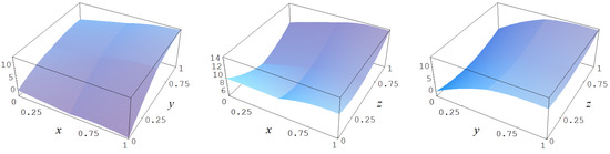
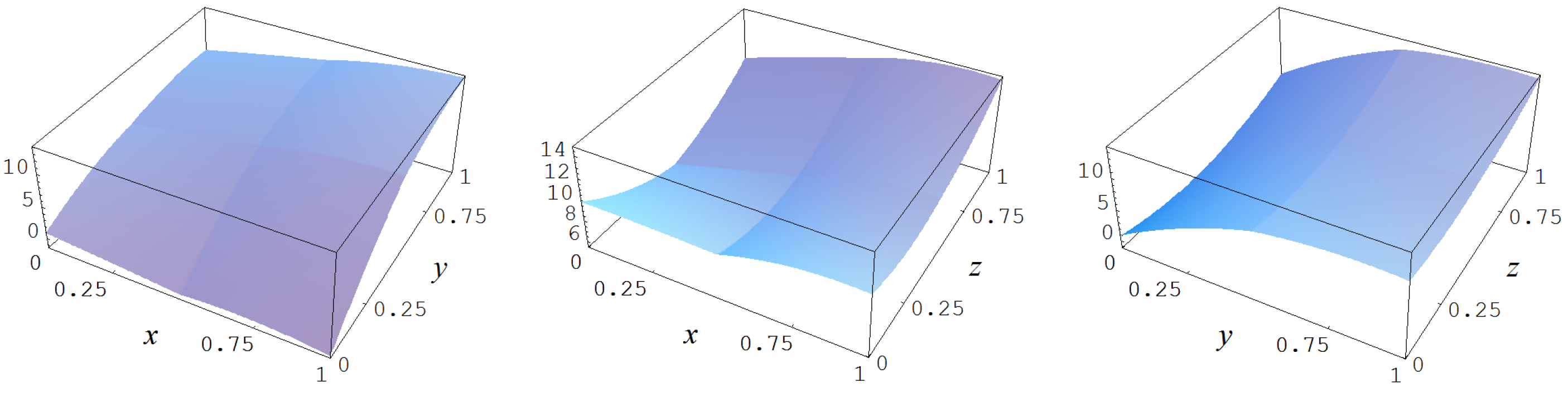
Figure A22.
Example of the trivariate C-spline model for (A17), for , , and , respectively.
Figure A22.
Example of the trivariate C-spline model for (A17), for , , and , respectively.
References
- Jaynes, E.T. Prior Probabilities. IEEE Trans. Syst. Sci. Cybern. 1968, 4, 227–241. [Google Scholar] [CrossRef]
- Van Erp, H.R.N.; Linger, R.O.; van Gelder, P.H.A.J.M. Deriving Proper Uniform Priors for Regression Coefficients, Part II. AIP Conf. Proc. 2011, 1305, 101. [Google Scholar]
- Skilling, J. This Physicist’s View of Gelman’s Bayes. Bayesian Anal. 2008. Available online: http://www.stat.columbia.edu/gelman/stuff_for_blog/rant2.pdf (accessed on 27 April 2017).
- Van Erp, H.R.N.; van Gelder, P.H.A.J.M. Deriving Proper Uniform Priors for Regression Coefficients. In Bayesian Inference and Maximum Entropy Methods in Science and Engineering; Mohammad-Djafari, A., Bercher, J., Bessiere, P., Eds.; American Institute of Physics: College Park, MD, USA, 2012; pp. 101–106. [Google Scholar]
- Van Erp, H.R.N.; Linger, R.O.; van Gelder, P.H.A.J.M. Constructing Cartesian Splines. arXiv, 2014; arXiv:1409.5955v1. [Google Scholar]
- Zellner, A. An Introduction to Bayesian Inference in Econometrics; J. Wiley & Sons, Inc.: New York, NY, USA, 1971. [Google Scholar]
- MacKay, D.J.C. Information Theory, Inference, and Learning Algorithms; Cambridge University Press: Cambridge, UK, 2003. [Google Scholar]
- Knuth, K.H.; Habeck, M.; Malakar, N.K.; Mubeen, A.M.; Placek, B. Bayesian Evidence and Model Selection. arXiv, 2014; arXiv:1411.3013v1. [Google Scholar]
- Bretthorst, L.G. Bayesian Spectrum Analysis and Parameter Estimation; Springer: New York, NY, USA, 1988; Volume 48. [Google Scholar]
- Lay, D.C. Linear Algebra and Its Applications; Addison-Wesley Publishing Company: Boston, MA, USA, 2000. [Google Scholar]
- Jaynes, E.T. Probability Theory: The Logic of Science; Cambridge University Press: Cambridge, UK, 2003. [Google Scholar]
- Lindgren, B.W. Statistical Theory; Chapman & Hall, Inc.: New York, NY, USA, 1993. [Google Scholar]
- Kass, R.; Raftery, A. Bayes Factors. J. Am. Stat. Assoc. 1995, 90, 773–795. [Google Scholar] [CrossRef]
- Linger, R.O.; van Erp, H.R.N.; van Gelder, P.H.A.J.M. Constructing Explicit B-Spline Bases. arXiv, 2014; arXiv:1409.3824v1. [Google Scholar]
- Ivakhenko, A.G. Group Method of Data Handling—A Rival of the Method of Stochastic Approximation. Sov. Autom. Control 1966, 13, 43–71. [Google Scholar]
- Awanou, G. Energy Methods in 3D Spline Approximations of Navier-Stokes Equations. Ph.D. Thesis, University of Georgia, Athens, GA, USA, 2003. [Google Scholar]
- MacKay, D.J.C. Bayesian Non-Linear Modelling with Neural Networks. University of Cambridge Programme for Industry, Modelling Phase Transformations in Steels, 1995. Available online: http://citeseerx.ist.psu.edu/viewdoc/summary?doi=10.1.1.48.1325 (accessed on 27 April 2017).
© 2017 by the authors. Licensee MDPI, Basel, Switzerland. This article is an open access article distributed under the terms and conditions of the Creative Commons Attribution (CC BY) license (http://creativecommons.org/licenses/by/4.0/).