3.1. Stabilizer Representation
From Theorem 1, propagation of the stabilizer state
can be represented by considering the state’s Wigner function:
. In this way,
and
specify a linear system of equations in terms of
and
. The first
n rows of
are the coefficients of
in
and the last
n rows of
are the coefficients of
in
:
The Kronecker delta function sets this linear system of equations equal to
. In this way, an affine map—a linear transformation displaced from the origin by
—is defined. This system of equations must be updated after every unitary propagation and measurement.
Since the Wigner functions
of stabilizer states propagate under
as
, it follows that
(The importance of vector
and when it must be updated will become evident when we consider random measurements.) Hence, after
n operations
,
,
…,
,
The matrices are ordered chronologically left-to-right instead of right-to-left.
Since
is symplectic,
where
Thus, the the stability matrices
for
,
and
given in Equations (
12)–(
14) differ from their inverses only by sign changes in their off-diagonal elements:
and
We assume the quantum state is initialized in the computational basis state
and so initially we should set
and
. The initial stabilizer state is
. However, it will become clear when we discuss measurements that it is practically useful to instead set
thereby setting
—not a true Wigner function. This new matrix
is equivalent to the last matrix if the first
n rows in
and
are ignored—the same as ignoring
. In fact, we have two Wigner functions here: one defined by the first
n rows and another by the last
n rows. We proceed in this manner, ignoring the first
n rows, until their usefulness becomes apparent to us.
For n qudits unitary propagation requires dits of storage to track and . More precisely, since is a matrix and is an -vector, dits of storage are necessary.
3.2. Unitary Propagation
contains the coefficients of the linear equations relating to . Each row is one equation relating or to . When manipulating rows of we shall refer to the linear equations that these rows define.
Examining Equations (
19)–(
21), we see that the inverse stability matrices of the generator gates
,
and
are the sum of an identity matrix and a matrix with a finite number of non-zero off-diagonal elements. The number of these off-diagonal elements is independent of the number of qudits,
n. Hence, multiplying
with a new stability matrix in Equation (
16) and evaluating the matrix multiplication is equivalent to performing a finite number of
n-vector dot products and so requires
operations. Therefore, keeping track of propagation of stabilizer states by Clifford gates can be simulated with
operations.
Let us examine these unitary operations more closely. Defining ⊕ and ⊖ to be mod d addition and subtraction respectively, we find:
Phase gate on qudit i (). For all , set .
Hadamard gate on qudit i (). For all , negate mod d, and then swap and .
CNOT from control i to target j (). For all , set and .
This confirms that unitary propagation in this scheme requires operations.
3.3. Measurement
The outcome of a measurement
on a stabilizer state can be either random or deterministic. As described above, the bottom half of
defines
for
, each of which is a linear combination of
and
. The entries in the
th row of
give the coefficient of
and
in
for
. If the coefficient of
in any
is non-zero then the measurement
will be random. If all coefficients of
are zero for
, then the measurement of
will be deterministic. This can be seen from the fact that if our stabilizer state
is an eigenstate of
, then
for some
and (discrete) Wigner functions do not change under a global phase. Thus, measuring
leaves the Wigner function of
invariant if the measurement is deterministic. Since
is a boost operator that increments the momentum of a state by one, its effect on the linear system of equations specified by the Wigner function is:
Thus, if the lower half of the
ith column of
is zero, then
leaves the Wigner function invariant (and so the measurement is deterministic). Verifying that these coefficients are all zero takes
operations for each
.
In other words, to see if a given measurement of is random or deterministic, a search must be performed for non-zero elements. If such a non-zero element exists, then the measurement is random since it means that the final momentum of qudit i affects the state of the stabilizer and so its position must be undetermined (by Heisenberg’s uncertainty principle). If no such finite element exists, then the measurement is deterministic. We now describe the algorithm in detail for these two cases:
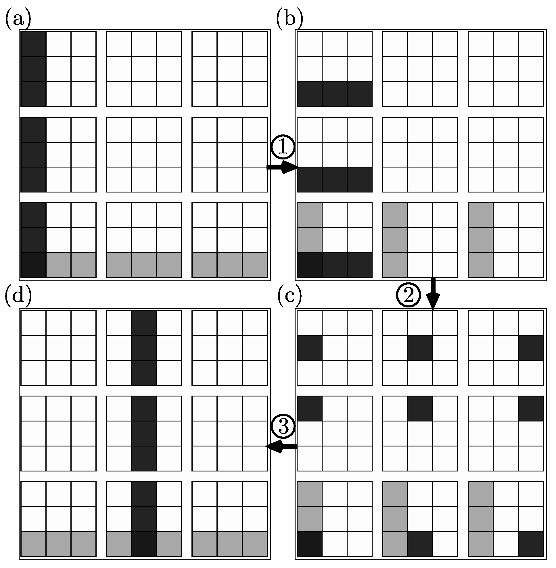
Case 1: Random Measurement
Let the th row in the bottom half of have a non-zero entry in the ith column, . Since the random measurement will project qudit i onto a position state, we will replace the th row with (the uniformly random outcome of this measurement). After this projection onto a position state, none of the other qudits’ positions should depend on qudit i’s momentum, . To accomplish this, before we replace row , we solve its equation for and substitute every instance of in the linear system of equations with this solution. As a result, every equation will no longer depend on and we can go ahead and replace the th row with .
There is one more thing to do, which will be important for deterministic measurements: replace the jth row with the old th row. This sets , which becomes the only remaining equation explicitly dependent on . In other words, , similar to the beginning when we set by setting . However, now we also preserve any dependence has on the other qudits incurred during unitary propagation. In other words, we preserve ’s dependence upon the other qudits, but only in the Wigner function specified by the top n rows, which we ignore otherwise.
After replacing the equation specified by row of and with a randomly chosen measurement outcome (i.e., ), the identification of rows and are exchanged, so that the former now specifies while the latter specifies . has also been updated by replacing the jth row in the first half of , with the th row we just changed. Again, this row now describes while the ith row now specifies . Overall, this takes operations since we are replacing rows with entries.
Case 2: Deterministic Measurement
Since the measurement is deterministic,
and
do not change. The
n equations specified by the bottom half of
can be used to solve for
—the deterministic measurement outcome. In general, this can also be done by inverting
and evaluating
for
. Aaronson and Gottesman themselves noted that such a matrix inversion is possible, but practically takes
operations. (However, we are not certain if Aaronson and Gottesman were referring to the
matrix corresponding to the
part of their tableau when they discuss matrix inversion in [
2].)
Fortunately, there is another method that scales as
and requires use of the
n equations represented by the top
n rows of
, which were included in our description by setting
. The linear system of
n equations represented by
can be written as
where we are interested in linear combinations of the bottom half,
, to solve for the measurement outcome
:
where
.
Lemma 1. The coefficient in front of in the row of that specifies , , is equal to the coefficient in front of that makes up in Equation (26). Equivalently, Proof. Under evolution under the Clifford group operators,
since
is symplectic. This means that we can express the matrix inversion as follows:
Therefore,
, and so
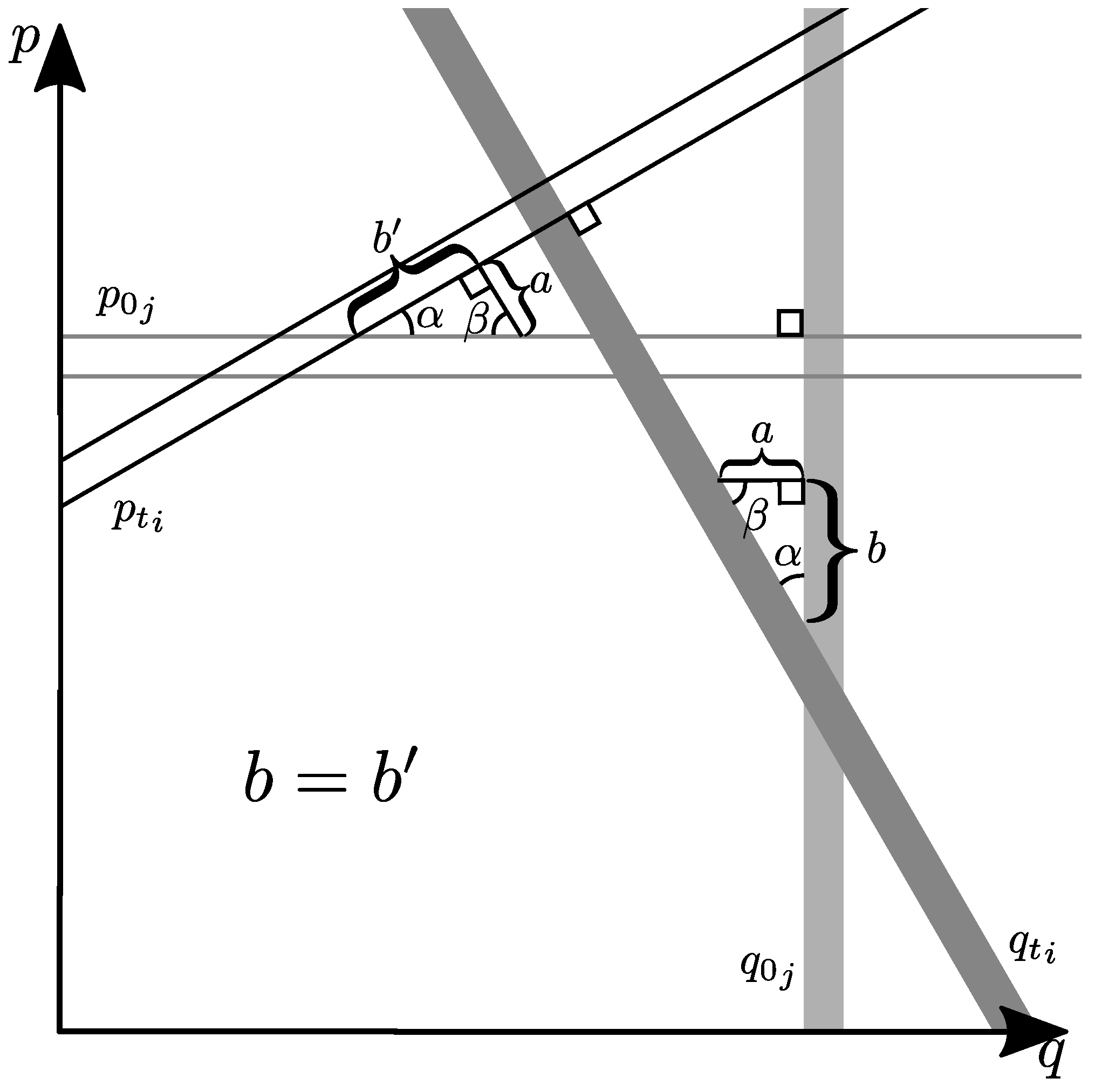
This property can also be seen in the drawing of phase space shown in
Figure 1. There, initial perpendicular
and
manifolds are drawn along with harmonically evolved
and
manifolds, which remain perpendicular to each other and make an angle
to the first
and
manifolds, respectively. The projection of
onto
can be represented as the length
b of a right triangle’s adjacent side to the angle
, with an opposite side set to some length
a. The projection of
onto
is similarly represented by the length
of a right triangle’s adjacent side to the angle
, with an opposite side also set to length
a. It follows that the third angle
in both triangles must be the same, and so by the law of sines
Therefore,
and so these two projections are equal to one another. In the discrete Weyl phase space such manifolds must lie along grid phase points and obey the periodicity in
and
, but the premise is the same. ☐
Overall, the procedure outlined in Lemma 1 for deterministic measurements takes
operations since Equation (
27) is a sum of
vectors made up of
components. Therefore, the overall measurement protocol takes
operations. Note that this formulation of the algorithm shows that it is the symplectic structure on phase space and the linear transformation under harmonic evolution that allows the inversion (Equation (32)) to be performed efficiently.


