Group-Constrained Maximum Correntropy Criterion Algorithms for Estimating Sparse Mix-Noised Channels

Abstract

A group-constrained maximum correntropy criterion (GC-MCC) algorithm is proposed on the basis of the compressive sensing (CS) concept and zero attracting (ZA) techniques and its estimating behavior is verified over sparse multi-path channels. The proposed algorithm is implemented by exerting different norm penalties on the two grouped channel coefficients to improve the channel estimation performance in a mixed noise environment. As a result, a zero attraction term is obtained from the expected $l_0$ and $l_1$ penalty techniques. Furthermore, a reweighting factor is adopted and incorporated into the zero-attraction term of the GC-MCC algorithm which is denoted as the reweighted GC-MCC (RGC-MMC) algorithm to enhance the estimation performance. Both the GC-MCC and RGC-MCC algorithms are developed to exploit well the inherent sparseness properties of the sparse multi-path channels due to the expected zero-attraction terms in their iterations. The channel estimation behaviors are discussed and analyzed over sparse channels in mixed Gaussian noise environments. The computer simulation results show that the estimated steady-state error is smaller and the convergence is faster than those of the previously reported MCC and sparse MCC algorithms.

1. Introduction

With the rapid rise of various wireless technologies, wireless transmissions have been widely developed in various fields such as mobile communications and satellite communication systems [1,2]. However, the signal might be distorted due to the diffraction, refraction, reflection or deviation from obstacles such as buildings, mountains and so on, resulting in transmission delays and other adverse effects. In the wireless communication transmission channels, the selective fading will lead to delays, which is also known as multi-path effects. In fact, the multi-path channel is always sparse [3,4,5], which means that most of the channel impulse response (CIR) coefficients are small while only a few of them are large in magnitude [6]. Since the CIR is sparse, many channel estimation algorithms have been presented to utilize this characteristic to improve the communication quality [2,7]. It is known that the adaptive filtering (AF) algorithm can be used for implementing channel estimation. Thus, various AF algorithms have been reported and used for channel estimation. Among these AF algorithms, the most typical algorithm is the least mean square (LMS) which is invented by B. Widrow. The LMS algorithm has been extensively investigated in channel estimation and noise cancellation owing to its simple implementation, high stability and fast convergence speed [4,8]. However, its performance is not satisfactory for sparse channel estimation with a low signal to noise ratio (SNR).

Recently, the compressive sampling (CS) concept has been introduced into AF algorithms to handle the sparse signals [9,10]. After that, Y. Chen et al. put forward to the zero attracting LMS (ZA-LMS) and reweighting ZA-LMS (RZA-LMS) algorithms [11]. ZA-LMS and RZA-LMS algorithms are implemented by integrating $l_1$-norm and reweighting $l_1$-norm into the LMS’s cost function, respectively. These two algorithms achieve lower steady-error and faster convergence speed than that of the basic LMS algorithm for handling sparse signals owing to the constructed zero attractors. Moreover, $l_0$-norm and $l_p$-norm have also been employed and introduced into the LMS’s cost function to improve the performance of the ZA- and RZA-LMS algorithms in the sparse signal processing area [12,13,14,15,16]. All of those norm-constrained LMS algorithms can effectively exploit sparse characteristics of the in-nature sparse channels. However, they have a common drawback, i.e., their sensitivity to the input signal scaling (ISS) and noise interferences. In order to reduce the effects of the ISS, several improved AF algorithms have been presented by using high order error criteria or mixed error norms such as least mean fourth (LMF), least mean squares-fourth (LMS/F) and so on [17,18,19,20]. Similarly, their related sparse forms have also been developed based on the above mentioned norm penalties [17,21,22,23,24,25,26,27]. However, those AF algorithms and their related sparse forms are not good enough for dealing with the sparse channel under non-Gaussian or mixed noise environments.

In recent years, information theoretic quantities were used for implementing cost function in adaptive systems. The effective entropy-based AF algorithms include the maximum correntropy criterion (MCC) and the minimum error entropy (MEE) [28,29,30,31,32]. In [28], it is shown that the MEE is more complex than the MCC algorithm in the computational overhead. Therefore, the MCC algorithm has been extensively developed in non-Gaussian environments [29,31,32]. Furthermore, the MCC has low complexity which is nearly the same as that of the LMS-like algorithms. However, the performance of the MCC algorithm may be degraded for sparse signal processing. In order to enhance the MCC algorithm for handling sparse signal and sparse system identification, $l_1$-norm and reweighting $l_1$-norm constraints have been exerted on the channel coefficient vector and integrated into the MCC’s cost function. Similar to the ZA-LMS and RZA-LMS algorithms, the zero attracting MCC (ZA-MCC) and reweighting ZA-MCC (RZA-MCC) algorithms [33] were obtained within the zero attracting framework. Then, the normalized MCC (NMCC) algorithm was also presented [34,35] by referring to the normalized least mean square (NLMS) algorithm. Recently, W. Ma proposed a correntropy-induced metric (CIM) penalized MCC algorithm in [33], and Y. Li presented a soft parameter function (SPF) constrained MCC algorithm [34]. The CIM and SPF are also one kind of $l_0$-norm approximation to form sparse MCC algorithms, and the SPF-MCC is given in the appendix. As for these improved MCC algorithms, the $l_0$-norm, CIM and SPF penalties are incorporated into the MCC’s cost function to devise desired zero attractors. In the ZA-MCC algorithm, the zero attractor gives uniform penalty on all the channel coefficients, while the $l_0$-norm approximation MCC algorithms will increase the complexity.

In this paper, a group-constrained maximum correntropy criterion (GC-MCC) algorithm based on the CS concept and zero attracting (ZA) techniques is proposed in order to fully exploit the sparseness characteristics of the multi-path channels. The GC-MCC algorithm is derived by incorporating a non-uniform norm into the MCC’s cost function and the non-uniform norm is split into two groups according to the mean of the magnitudes of the channel coefficients. For the large channel coefficients group, the $l_0$-norm penalty is used, while the $l_1$-norm penalty is implemented for the small channel group. Then, a reweighting technique is utilized in the GC-MCC algorithm to develop the reweighted GC-MCC (RGC-MCC) algorithm. The performance of the GC- and RGC-MCC algorithms is evaluated and discussed for estimating mix-noised sparse channels. The GC- and RGC-MCC algorithms achieve superior performance in both steady-error and convergence for sparse channel estimations with different sparsity levels. Simulation results show that the GC- and RGC-MCC algorithms can effectively enhance the sparse channel estimation by using the proposed group constraints and can provide smaller steady-state errors and faster convergence for application in a mixed noise environment.

The structure of this paper is summarized as follows. In Section 2, the MCC and its related sparse algorithms are briefly reviewed. Section 3 introduces the GC-MCC and RGC-MCC algorithms, and mathematically derives them. In Section 4, simulations that show the effectiveness of the proposed GC-MCC and RCG-MCC algorithms are presented. Finally, our work is summarized in Section 5.

2. Review of the MCC and Its Related Sparse Algorithms

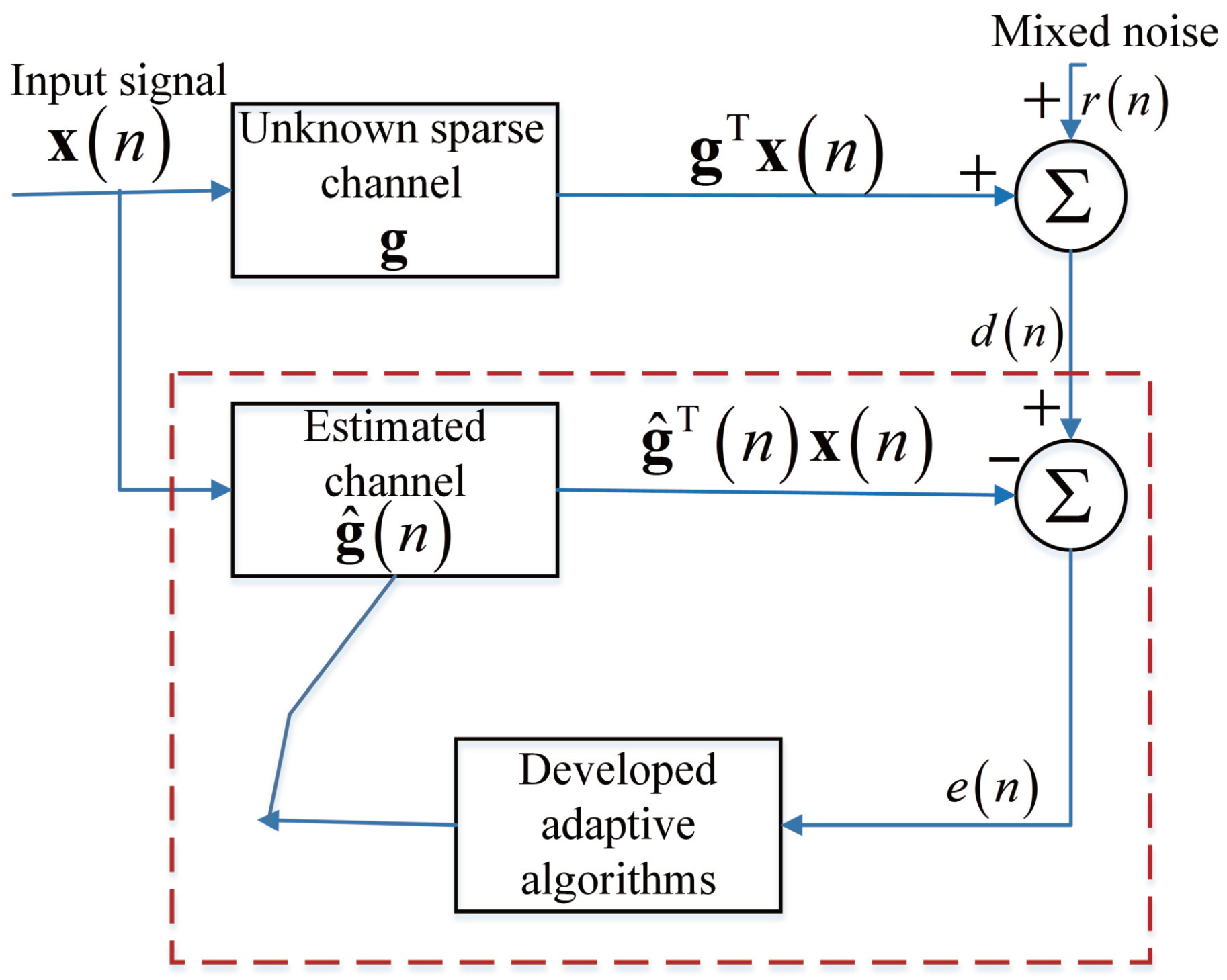
We consider a typical channel estimation system based on the MCC algorithm, which is given in Figure 1. $\mathbf{x}\left(n\right)$ is the input training signal with a length of M, which is surveyed to an unknown sparse channel whose vector form is $\mathbf{g}={\left[g_1,g_2,\dots ,g_M\right]}^{{}^T}$. As a sparse channel, most of the channel coefficients in the unknown sparse channel $\mathbf{g}$ are zeros or near-zeros. Herein, we use K to represent the number of nonzero coefficients in the unknown sparse channel $\mathbf{g}$. Then, the desired signal can be written as

$$d\left(n\right)={\mathbf{g}}^T\mathbf{x}\left(n\right)+r\left(n\right),$$

(1)

where $r\left(n\right)$ is a mixed Gaussian noise which is independent of the input training signal $\mathbf{x}\left(n\right)$. Moreover, the instantaneous estimation error at n-th iteration is defined as

$$e\left(n\right)=d\left(n\right)-{\widehat{\mathbf{g}}}^T\left(n\right)\mathbf{x}\left(n\right),$$

(2)

where $\widehat{\mathbf{g}}\left(n\right)$ denotes the estimated channel vector. The MCC-based channel estimation is to obtain the minimization of the iterative instantaneous estimation error $e\left(n\right)$, and hence, we can estimate the unknown sparse channel $\mathbf{g}$.

Figure 1. Structure diagram of sparse channel estimation.

The MCC algorithm is using the localized similarity to solve the following problem

$$\begin{array}{c}\min \frac{1}{2}{∥\widehat{\mathbf{g}}\left(n+1\right)-\widehat{\mathbf{g}}\left(n\right)∥}^2\hfill \\ \mathrm{subject}\mathrm{to}\widehat{e}\left(n\right)=\left[1-\alpha \exp \left(-\frac{e^2\left(n\right)}{2{\sigma }^2}\right)\right]e\left(n\right)\hfill \end{array},$$

(3)

where $\widehat{e}\left(n\right)=d\left(n\right)-{\widehat{\mathbf{g}}}^T\left(n+1\right)\mathbf{x}\left(n\right)$, and $\sigma >0$ is a trade off parameter. Additionally, ${∥•∥}^2$ represents the Euclidean norm [36], and $\alpha ={\beta }_{\mathrm{MCC}}{∥\mathbf{x}\left(n\right)∥}^2$, where ${\beta }_{\mathrm{MCC}}$ is the step-size of the MCC algorithm. Based on Equation (3), we can write MCC’s cost function as

$$J_0\left(n\right)=\frac{1}{2}{∥\widehat{\mathbf{g}}\left(n+1\right)-\widehat{\mathbf{g}}\left(n\right)∥}^2+{\lambda }_{\mathrm{MCC}}\left(\widehat{e}\left(n\right)-\left[1-\alpha \exp \left(-\frac{e^2\left(n\right)}{2{\sigma }^2}\right)\right]e\left(n\right)\right),$$

(4)

where ${\lambda }_{\mathrm{MCC}}$ is the multiplier parameter. By utilizing the Lagrange multiplier method (LMM), we can obtain the partial derivatives of $\widehat{\mathbf{g}}\left(n+1\right)$ and ${\lambda }_{\mathrm{MCC}}$ in Equations (5) and (6)

$$\widehat{\mathbf{g}}\left(n+1\right)-\widehat{\mathbf{g}}\left(n\right)-{\lambda }_{\mathrm{MCC}}\mathbf{x}\left(n\right)=0,$$

(5)

$$\widehat{e}\left(n\right)-\left[1-\alpha \exp \left(-\frac{e^2\left(n\right)}{2{\sigma }^2}\right)\right]e\left(n\right)=0.$$

(6)

Then, we get ${\lambda }_{\mathrm{MCC}}$

$${\lambda }_{\mathrm{MCC}}=\alpha \frac{\exp \left(-\frac{e^2\left(n\right)}{2{\sigma }^2}\right)e\left(n\right)}{{∥\mathbf{x}\left(n\right)∥}^2}.$$

(7)

Substituting (7) into (5), the updating equation with the vector formed of the MCC algorithm is

$$\widehat{\mathbf{g}}\left(n+1\right)=\widehat{\mathbf{g}}\left(n\right)+{\beta }_{\mathrm{MCC}}\exp \left(-\frac{e^2\left(n\right)}{2{\sigma }^2}\right)e\left(n\right)\mathbf{x}\left(n\right).$$

(8)

It can be seen that the recursion of the MCC algorithm is similar to the LMS algorithm, except the exponential term. Similarly, the MCC algorithm does not utilize the intrinsic sparsity property of the sparse channels. Motivated by the ZA-LMS and RZA-LMS algorithms, sparse MCC algorithms have been presented and they are named as zero attracting MCC (ZA-MCC) and reweighting ZA-MCC (RZA-MCC) [33]. For the ZA-MCC algorithm, it is implemented by integrating a $l_1$-norm into MCC’s cost function, and solving [33]

$$\begin{array}{c}\min \frac{1}{2}{∥\widehat{\mathbf{g}}\left(n+1\right)-\widehat{\mathbf{g}}\left(n\right)∥}^2+{\theta }_{\mathrm{ZA}}{∥\widehat{\mathbf{g}}\left(n+1\right)∥}_1\hfill \\ \mathrm{subject}\mathrm{to}\widehat{e}\left(n\right)=\left[1-\alpha \exp \left(-\frac{e^2\left(n\right)}{2{\sigma }^2}\right)\right]e\left(n\right)\hfill \end{array},$$

(9)

where ${∥•∥}_1$ is the $l_1$-norm, and a regularization parameter ${\theta }_{\mathrm{ZA}}$ is used for controlling its ability. Based on the LMM, the ZA-MCC’s cost function is [33]

$$J_1\left(n\right)=\frac{1}{2}{∥\widehat{\mathbf{g}}\left(n+1\right)-\widehat{\mathbf{g}}\left(n\right)∥}^2+{\theta }_{\mathrm{ZA}}{∥\widehat{\mathbf{g}}\left(n+1\right)∥}_1+{\lambda }_{\mathrm{ZA}}\left(\widehat{e}\left(n\right)-\left[1-\alpha \exp \left(-\frac{e^2\left(n\right)}{2{\sigma }^2}\right)\right]e\left(n\right)\right),$$

(10)

where ${\lambda }_{\mathrm{ZA}}$ is the multiplier parameter of the ZA-MCC algorithm. By using LMM, the updating Equation of the ZA-MCC algorithm is [33]

$$\widehat{\mathbf{g}}\left(n+1\right)=\widehat{\mathbf{g}}\left(n\right)+{\beta }_{\mathrm{ZA}}\exp \left(-\frac{e^2\left(n\right)}{2{\sigma }^2}\right)e\left(n\right)\mathbf{x}\left(n\right)-{\theta }_{\mathrm{ZA}}\mathrm{sgn}\left[\widehat{\mathbf{g}}\left(n\right)\right],$$

(11)

where ${\theta }_{\mathrm{ZA}}$ is a zero attracting ability controlling parameter that is used for giving a tradeoff between the estimation error and $l_1$-norm constraint, and ${\beta }_{\mathrm{ZA}}$ is the step-size of the ZA-MCC algorithm. However, we noticed that the zero attraction term $-{\theta }_{\mathrm{ZA}}\mathrm{sgn}\left[\widehat{\mathbf{g}}\left(n\right)\right]$ uniformly attracts all the channel coefficients to zero. Therefore, its performance might be degraded when it deals with less sparse channels. Then, a reweighting factor is introduced into the zero attraction term $-{\theta }_{\mathrm{ZA}}\mathrm{sgn}\left[\widehat{\mathbf{g}}\left(n\right)\right]$, resulting in a RZA-MCC algorithm whose updating equation is [33]

$$\widehat{\mathbf{g}}\left(n+1\right)=\widehat{\mathbf{g}}\left(n\right)+{\beta }_{\mathrm{RZA}}\exp \left(-\frac{e^2\left(n\right)}{2{\sigma }^2}\right)e\left(n\right)\mathbf{x}\left(n\right)-{\theta }_{\mathrm{RZA}}\frac{\mathrm{sgn}\left[\widehat{\mathbf{g}}\left(n\right)\right]}{1+\epsilon \left|\widehat{\mathbf{g}}\left(n\right)\right|},$$

(12)

where $\epsilon$, ${\theta }_{\mathrm{RZA}}$ and ${\beta }_{\mathrm{RZA}}$ are the reweighting controlling factor, zero attraction controlling parameter and the RZA-MCC’s step-size, respectively. It can be seen from the upgrading equation that $-{\theta }_{\mathrm{RZA}}\frac{\mathrm{sgn}\left[\widehat{\mathbf{g}}\left(n\right)\right]}{1+\epsilon \left|\widehat{\mathbf{g}}\left(n\right)\right|}$ acts as the zero attractor which exerts different zero attraction to the channel coefficients that depends on their magnitudes.

3. The Proposed Group-Constrained Sparse MCC Algorithms

From the above discussion, we found that the zero attractor $-{\theta }_{\mathrm{ZA}}\mathrm{sgn}\left[\widehat{\mathbf{g}}\left(n\right)\right]$ is realized by incorporating the $l_1$-norm penalty in the MCC’s cost function, and it can speed up the convergence and reduce the channel estimation error. Moreover, the $l_0$-norm-constrained MCC algorithm can further improve the performance since the $l_0$-norm can count the number of the non-zero channel coefficients. However, the complexity is significantly increased due to the calculation of the $l_0$-norm approximation and its constraint. In order to fully exploit the sparsity property of the multi-path channel, we propose a group-constrained MCC algorithm by exerting the $l_0$-norm penalty on the group of large channel coefficients and forcing the $l_1$-norm penalty on the group of small channel coefficients. Herein, a non-uniform norm is used to split the non-uniform penalized algorithms into a large group and a small group, and the non-uniform norm is defined as [37,38]

$${∥\widehat{\mathbf{g}}\left(n\right)∥}_p^p=\sum _{i=1}^M{\left|{\widehat{\mathrm{g}}}_i\left(n\right)\right|}^p,0\le p\le 1,$$

(13)

which is a $l_0$-norm when $p\to 0$

$$\underset{p\to 0}{lim}{∥\widehat{\mathbf{g}}\left(n\right)∥}_p^p={∥\widehat{\mathbf{g}}\left(n\right)∥}_0,$$

(14)

and it is a $l_1$-norm when p is infinitely close to 1

$$\underset{p\to 1}{lim}{∥\widehat{\mathbf{g}}\left(n\right)∥}_p^p={∥\widehat{\mathbf{g}}\left(n\right)∥}_1.$$

(15)

Herein, the uniform-norm given in Equation (13) is a variable norm which is controlled by the parameter p. When p is very close to zero, the proposed norm in Equation (13) can be regarded as a $l_0$-norm. As for $p=$ 1, the norm in Equation (13) is the $l_1$-norm. Then, the constructed non-uniform norm in Equation (13) is introduced into the MCC’s cost function to devise our proposed GC-MCC algorithm, and GC-MCC is to solve

$$\begin{array}{c}\min \frac{1}{2}{∥\widehat{\mathbf{g}}\left(n+1\right)-\widehat{\mathbf{g}}\left(n\right)∥}^2+{\theta }_{\mathrm{GC}}{∥\widehat{\mathbf{g}}(n+1)∥}_{p,M}^p\hfill \\ \mathrm{subject}\mathrm{to}\widehat{e}\left(n\right)=\left[1-\alpha \exp \left(-\frac{e^2\left(n\right)}{2{\sigma }^2}\right)\right]e\left(n\right)\hfill \end{array},$$

(16)

where ${∥\widehat{\mathbf{g}}(n+1)∥}_{p,M}^p$ is a kind of ${∥\widehat{\mathbf{g}}(n+1)∥}_p^p$, which uses a different value of p for each channel coefficient at M-th position in the sparse channels, here with the introduction of $\mathbf{p}=\left[p_1,p_2,\dots ,p_M\right]$, and ${\theta }_{\mathrm{GC}}$ is a regularization parameter. Then, the cost function of the GC-MCC algorithm is

$$J_{\mathrm{GC}}\left(n\right)=\frac{1}{2}{∥\widehat{\mathbf{g}}\left(n+1\right)-\widehat{\mathbf{g}}\left(n\right)∥}^2+{\theta }_{\mathrm{GC}}{∥\widehat{\mathbf{g}}(n+1)∥}_{p,M}^p+{\lambda }_{\mathrm{GC}}\left(\widehat{e}\left(n\right)-\left[1-\alpha \exp \left(-\frac{e^2\left(n\right)}{2{\sigma }^2}\right)\right]e\left(n\right)\right).$$

(17)

In Equation (17), ${\lambda }_{\mathrm{GC}}$ is a multiplier. Based on the LMM, the gradients of $J_{\mathrm{GC}}\left(n\right)$ with respect to $\widehat{\mathbf{g}}\left(n+1\right)$ and ${\lambda }_{\mathrm{GC}}$ are

$$\frac{\partial J_{\mathrm{GC}}\left(n\right)}{\partial \widehat{\mathbf{g}}\left(n+1\right)}=0,$$

(18)

and

$$\frac{\partial J_{\mathrm{GC}}\left(n\right)}{\partial {\lambda }_{\mathrm{GC}}}=0.$$

(19)

Then, we can get

$${\widehat{\mathrm{g}}}_i\left(n+1\right)={\widehat{\mathrm{g}}}_i\left(n\right)-{\theta }_{\mathrm{GC}}\frac{p_i·\mathrm{sgn}\left[{\widehat{\mathrm{g}}}_i\left(n+1\right)\right]}{{\left|{\widehat{\mathrm{g}}}_i\left(n+1\right)\right|}^{1-p_i}}+{\lambda }_{\mathrm{GC}}{x}_i\left(n\right),$$

(20)

and

$$\widehat{e}\left(n\right)=\left[1-\alpha \exp \left(-\frac{e^2\left(n\right)}{2{\sigma }^2}\right)\right]e\left(n\right),$$

(21)

where $p_i$ is the i-th element of matrix $\mathbf{p}$. From Equations (20) and (21), we can obtain ${\lambda }_{\mathrm{GC}}$

$${\lambda }_{\mathrm{GC}}=\frac{\alpha \exp \left(-\frac{e^2\left(n\right)}{2{\sigma }^2}\right)e\left(n\right)+{\theta }_{\mathrm{GC}}\frac{p_i·\mathrm{sgn}\left[{\widehat{\mathrm{g}}}_i\left(n+1\right)\right]}{{\left|{\widehat{\mathrm{g}}}_i\left(n+1\right)\right|}^{1-p_i}}{x}_i^{\mathrm{T}}\left(n\right)}{{∥x_i\left(n\right)∥}^2}.$$

(22)

Substituting ${\lambda }_{\mathrm{GC}}$ into Equation (20), the updated equation of the proposed GC-MCC algorithm is

$${\widehat{\mathrm{g}}}_i\left(n+1\right)={\widehat{\mathrm{g}}}_i\left(n\right)+{\beta }_{\mathrm{GC}}\exp \left(-\frac{e^2\left(n\right)}{2{\sigma }^2}\right)e\left(n\right)x_i\left(n\right)-{\theta }_{\mathrm{GC}}\frac{p_i·\mathrm{sgn}\left[{\widehat{\mathrm{g}}}_i\left(n+1\right)\right]}{{\left|{\widehat{\mathrm{g}}}_i\left(n+1\right)\right|}^{1-p_i}}\left(1-\frac{x_i\left(n\right)x_i^{\mathrm{T}}\left(n\right)}{{∥x_i\left(n\right)∥}^2}\right)$$

(23)

where ${\beta }_{\mathrm{GC}}$ is a step-size for GC-MCC algorithm. It can be seen from Equation (23), the matrix $\mathbf{p}=\left[p_1,p_2,\dots ,p_M\right]$ can assign different $p_i$ to each channel coefficients. To better exert the $p_i$ to the channel coefficients, the channel coefficients are classified according to their magnitudes. From the measurement and the previous investigations of the sparse channels [2,6,7,10,11,12,13,14,15,16,21,22,23,24,26,27], we found that few channel coefficients are active non-zero ones, while most of the channel coefficients are inactive zero or near-zero ones. Thus, we propose a threshold to categorize the channel coefficients into two groups. Herein, a classify criterion which is used as the threshold is proposed based on the absolute value expectation of $\widehat{\mathbf{g}}\left(n\right)$ and it is defined as

$$y\left(n\right)=\mathrm{E}\left[\left|{\widehat{\mathrm{g}}}_i\left(n\right)\right|\right],\forall 1\le i<M.$$

(24)

Then, we categorize the channel coefficients into two groups in terms of the criterion in (24). When the channel coefficients ${\widehat{\mathrm{g}}}_i\left(n\right)>y\left(n\right)$, the channel coefficients belong to the “large” group, while ${\widehat{\mathrm{g}}}_i\left(n\right)<y\left(n\right)$, the channel coefficients are located in the “small” group. In fact, a threshold is proposed to split the variable norm into the “large” group and the “small” group, where the threshold is implemented using the mean of the estimated channel coefficients. If the channel coefficients are greater than this threshold, they are the “large” group. Otherwise, the channel coefficients belong to the “small” group when the channel coefficients are smaller than this threshold. For the “large” group, $l_0$-norm penalty is used to count the number of active channel coefficients, and $l_1$-norm penalty is adopted to uniformly attract inactive coefficients to zero for the “small” group. To effectively integrate these two groups into (23), we define [37]

$$f_i=\frac{\mathrm{sgn}\left[y\left(n\right)-\left|{\widehat{\mathrm{g}}}_i\left(n\right)\right|\right]+1}{2},\forall 1\le i<M.$$

(25)

Therefore, $f_i$ is set to be 0 when ${\widehat{\mathrm{g}}}_i\left(n\right)>y\left(n\right)$, while $f_i$ will be 1 for ${\widehat{\mathrm{g}}}_i\left(n\right)<y\left(n\right)$. Finally, the updated equation of the GC-MCC is

$${\widehat{\mathrm{g}}}_i\left(n+1\right)={\widehat{\mathrm{g}}}_i\left(n\right)+{\beta }_{\mathrm{GC}}\exp \left(-\frac{e^2\left(n\right)}{2{\sigma }^2}\right)e\left(n\right)x_i\left(n\right)-{\theta }_{\mathrm{GC}}{f}_i\mathrm{sgn}\left[{\widehat{\mathrm{g}}}_i\left(n+1\right)\right]\left(1-\frac{x_i\left(n\right)x_i^{\mathrm{T}}\left(n\right)}{{∥x_i\left(n\right)∥}^2}\right).$$

(26)

In Equation (26), $\frac{x_i\left(n\right)x_i^{\mathrm{T}}\left(n\right)}{{∥x_i\left(n\right)∥}^2}$ is far less than 1, so it can be ignored. Thus, the updating recursion of the GC-MCC algorithm is rewritten as

$$\widehat{\mathbf{g}}\left(n+1\right)=\widehat{\mathbf{g}}\left(n\right)+{\beta }_{\mathrm{GC}}\exp \left(-\frac{e^2\left(n\right)}{2{\sigma }^2}\right)e\left(n\right)\mathbf{x}\left(n\right)-{\theta }_{\mathrm{GC}}\mathbf{F}\mathrm{sgn}\left[\widehat{\mathbf{g}}\left(n\right)\right].$$

(27)

The last term $-{\theta }_{\mathrm{GC}}\mathbf{F}\mathrm{sgn}\left[\widehat{\mathbf{g}}\left(n\right)\right]$ is the proposed zero attraction term which exerts different zero attracting on the two grouped channel coefficients. We can see that both the $l_0$-norm and $l_1$-norm constraints are implemented on the channel coefficients in the GC-MCC algorithm, which is different from the ZA-MCC and $l_0$-MCC algorithms. For the GC-MCC channel estimation, our proposed zero attractor can distinguish the value of coefficients and categorize the channel coefficients into two groups. The proposed GC-MCC algorithm can achieve small steady-state error and fast convergence due to the term $-{\theta }_{\mathrm{GC}}\mathbf{F}\mathrm{sgn}\left[\widehat{\mathbf{g}}\left(n\right)\right]$.

To further enhance the performance of our proposed GC-MCC algorithm, a reweighting factor is introduced into the GC-MCC’s update equation to implement the RGC-MCC algorithm, which is similar to the RZA-LMS algorithm. Thus, the RGC-MCC’s updating equation is

$$\widehat{\mathbf{g}}\left(n+1\right)=\widehat{\mathbf{g}}\left(n\right)+{\beta }_{\mathrm{RGC}}\exp \left(-\frac{e^2\left(n\right)}{2{\sigma }^2}\right)e\left(n\right)\mathbf{x}\left(n\right)-{\theta }_{\mathrm{RGC}}\mathbf{F}\frac{\mathrm{sgn}\left[\widehat{\mathbf{g}}\left(n\right)\right]}{1+{\epsilon }_1\left|\widehat{\mathbf{g}}\left(n\right)\right|},$$

(28)

where ${\theta }_{\mathrm{RGC}}$ is the zero attraction controlling parameter, ${\epsilon }_1$ is the reweighting controlling parameter and ${\beta }_{\mathrm{RGC}}$ is a step-size of the RGC-MCC algorithm.

With the help of $-{\theta }_{\mathrm{RGC}}\mathbf{F}\frac{\mathrm{sgn}\left[\widehat{\mathbf{g}}\left(n\right)\right]}{1+{\epsilon }_1\left|\widehat{\mathbf{g}}\left(n\right)\right|}$, our proposed RGC-MCC algorithm can assign well different values $p_i$ to channel coefficients according to the magnitudes of the channel coefficients. Moreover, we can properly select the value of ${\epsilon }_1$ to obtain a better channel estimation performance. In fact, the proposed GC-MCC and RZA-GC-MCC algorithms are the extension of the ZA-MCC and RZA-MCC algorithms. However, the proposed GC-MCC and RGC-MCC are different with the proposed ZA-MCC, RZA-MCC and $l_0$-norm penalized MCC algorithms. Our contributions are summarized herein. The GC-MCC algorithm is realized by incorporating a variable norm in Equation (13) into the cost function of the traditional MCC algorithm, where the variable norm is controlled by the parameter p. To distinguish the large channel coefficients and the small channel coefficients, a mean of the estimated channel coefficients shown in Equation (24) is proposed to provide a threshold. Then, the variable norm is split into two groups by comparing the channel coefficients with the threshold. As a result, a large group is given when ${\widehat{g}}_i\left(n\right)>y\left(n\right)$, while a small group is created when ${\widehat{g}}_i\left(n\right)<y\left(n\right)$. For the channel coefficients in the large group, we use a $l_0$-norm to count the number of the non-zero channel coefficients. As for the channel coefficients in the small group, $l_1$-norm penalty is used for attracting the zero or near-zero channel coefficients to zero quickly. It is found that a norm penalty matrix with values in its diagonal is proposed in Equation (25) to implement the $l_0$ and $l_1$ in the GC-MCC algorithm, which is also different with the conventional $l_0$- and $l_1$- norm constraints. Then, we use a reweighting factor to enhance the zero attracting ability in the GC-MCC algorithm to generate the RGC-MCC algorithm. Both the GC-MCC and RGC-MCC algorithms are developed to exploit well the inherent sparseness properties of the multi-path channels due to the expected zero-attraction terms in their iterations. The channel estimation behaviors will be discussed over sparse channels in mixed Gaussian noise environments in the next section.

4. Computational Simulations and Discussion of Results

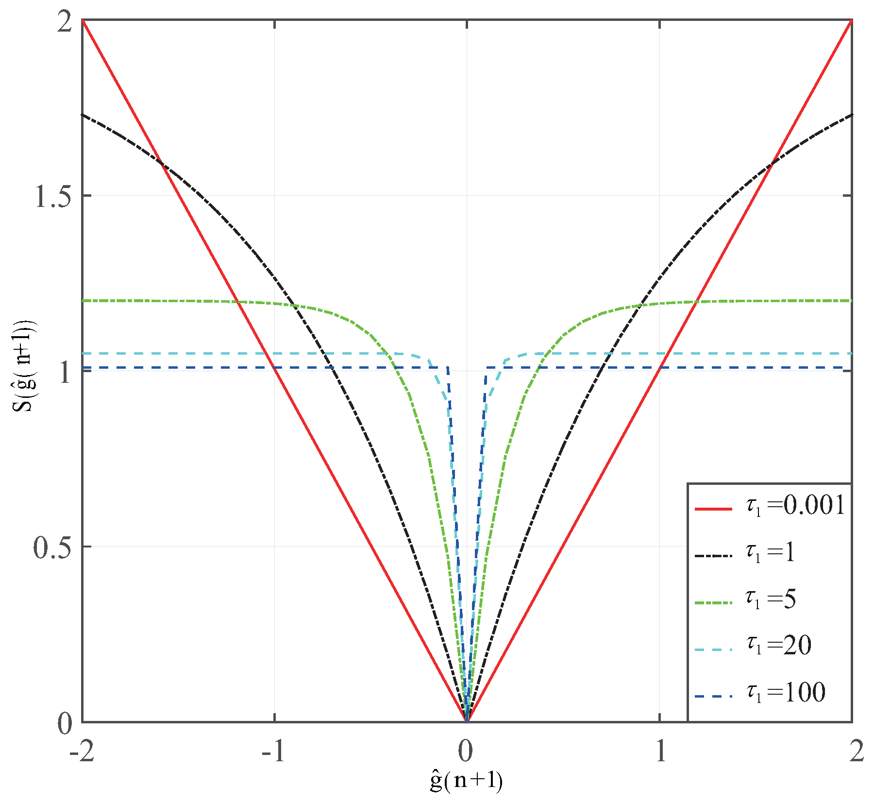
In this section, we will construct several experiments to verify the GC- and RGC-MCC’s channel estimation performance. The steady-state channel estimation error and the convergence are considered to give an evaluation of the proposed GC- and RGC-MCC algorithms. The results are also compared with the MCC, NMCC, ZA-, RZA- and SPF-MCC algorithms. From the discussion, we know that the CIM and SPF are $l_0$-norm approximations. Thus, we first set up an experiment to discuss the zero attraction ability of the CIM, SPF and $l_0$-norm approximation. The zero attraction ability of these $l_0$-norm approximations is shown in Figure 2. The related parameters in these $l_0$-norm approximations are ${\tau }_1$, ${\sigma }_1$ and $\tau$. It can be seen that the zero attraction ability of the SPF is close to the $l_0$-norm for larger ${\tau }_1$, while the zero attraction ability of the CIM approximates to $l_0$-norm when ${\sigma }_1$ is small. From these results, we found that the SPF can give an accurate approximation and can provide a better zero attraction when ${\tau }_1=\tau =5$ and ${\sigma }_1=0.05$. For ${\tau }_1=\tau =1$ and ${\sigma }_1=0.08$, the zero attraction ability of SPF is weak. However, it can give an adaption for a wider range of sparse channel estimation applications. It can be concluded that the zero attraction ability of the zero attractor produced by SPF is superior. Thus, we will choose SPF-MCC to give a comparison with our proposed GC-MCC and RGC-MCC algorithms in terms of the steady-state error and convergence.

Figure 2. Zero attraction ability of the zero attracting term produced by soft parameter function (SPF), $l_0$-norm and correntropy-induced metric (CIM) penalties.

All of the experiments are constructed under a mix-Gaussian noise environment, and the mixed noise model has been used in the previous study and is a better description of the real wireless communication environment. The mixed noise model is given by [34,36]

$$\left(1-\chi \right)N\left({\mu }_1,{\nu }_1^2\right)+\chi N\left({\mu }_2,{\nu }_2^2\right),$$

(29)

where $N\left({\mu }_i,{\nu }_i^2\right)\left(i=1,2\right)$ represent the Gaussian distribution, and parameters ${\mu }_i$, ${\nu }_i^2$ and $\chi$ are the means, variances and mixing parameter, respectively. In all the experiments, we set $\left({\mu }_1,{\mu }_2,{\nu }_1^2,{\nu }_2^2,\chi \right)=\left(0,0,0.05,20,0.05\right)$. The estimated performance of our proposed GC-MCC and RGC-MCC algorithms is given by mean square deviation (MSD), which is defined as

$$\mathrm{MSD}\left(\widehat{\mathbf{g}}\left(n\right)\right)=\mathrm{E}\left[{∥\mathbf{g}-\widehat{\mathbf{g}}\left(n\right)∥}^2\right].$$

(30)

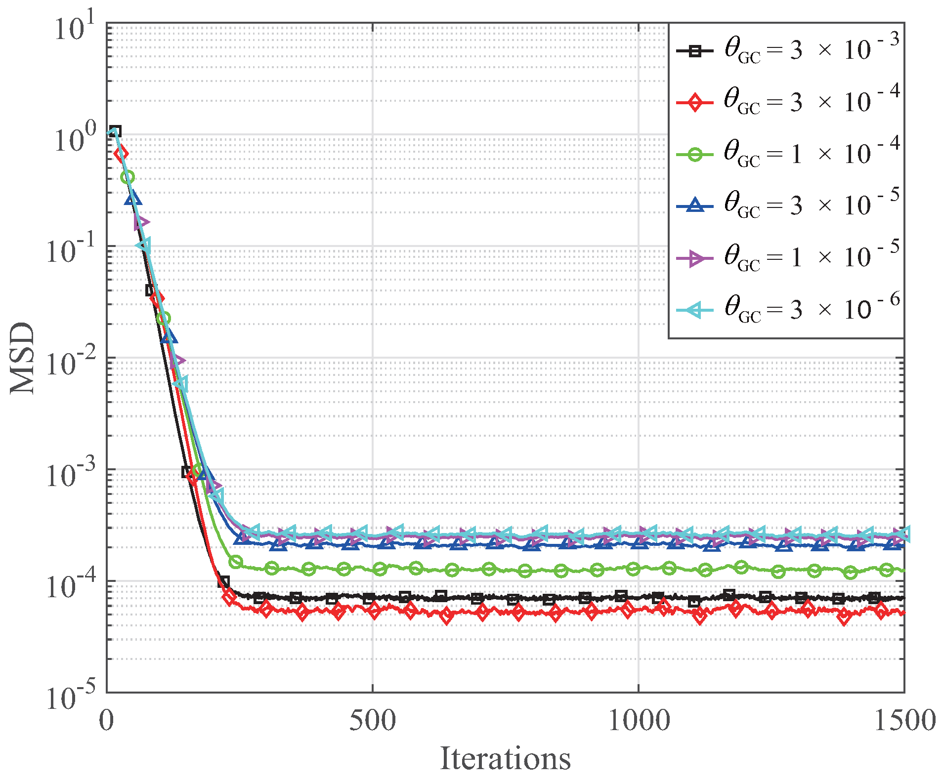
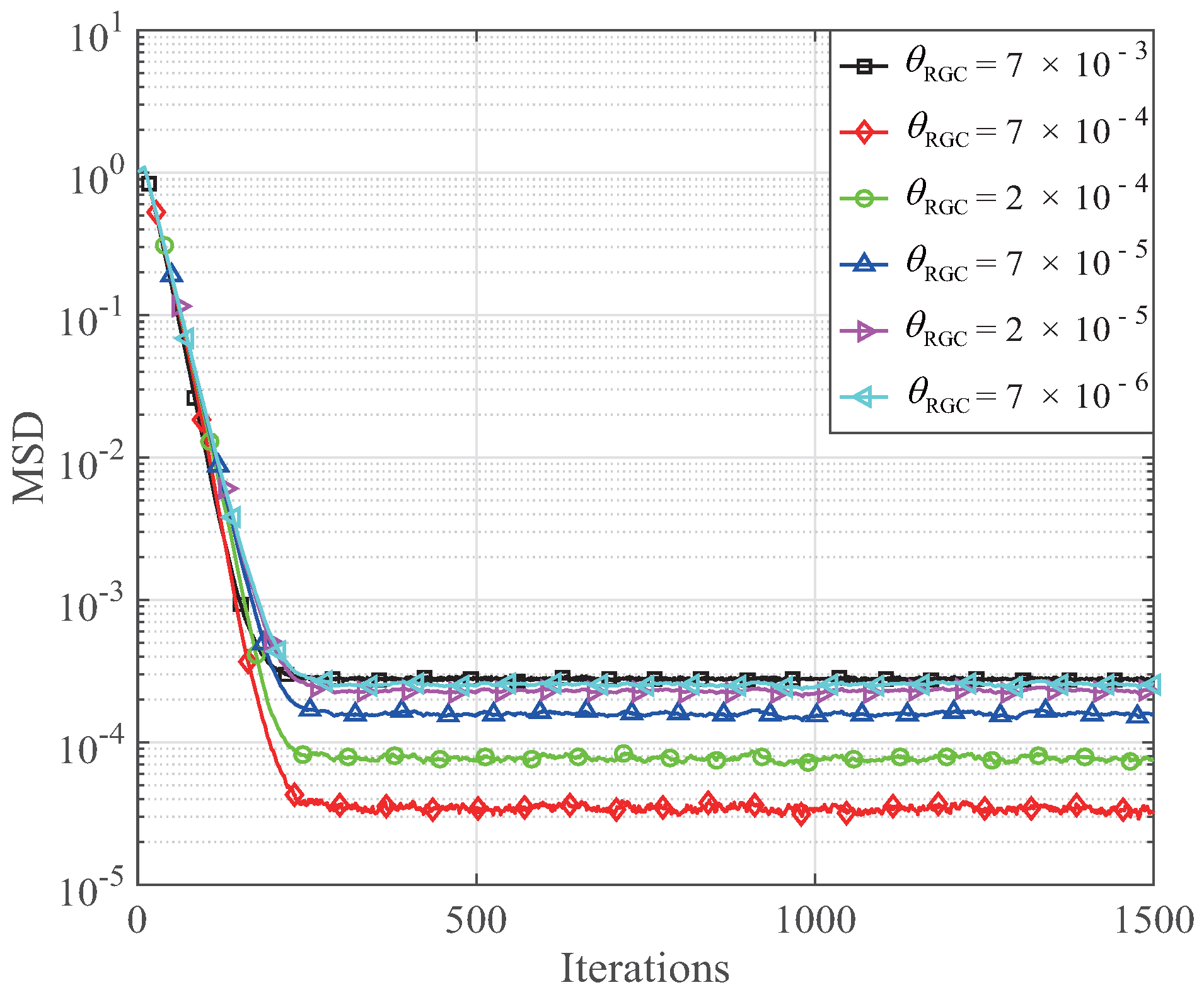
For all the simulations, 300 Monte Carlo runs are performed for obtaining each point in all mentioned algorithms. Herein, the total length of the unknown channel is $M=16$ and the number of the non-zero channel coefficients is K. The signal-to-noise ratio (SNR) is 30 dB. Those non-zero channel coefficients are randomly distributed within the length of the channel. Since the regularization parameters have an important effect on the performance of the proposed GC-MCC and RGC-MCC algorithms, the effects of regularization parameters ${\theta }_{\mathrm{GC}}$, ${\theta }_{\mathrm{RGC}}$ and ${\beta }_{\mathrm{GC}/\mathrm{RGC}}$ are investigated and given in Figure 3, Figure 4 and Figure 5.

Figure 3. Effects of ${\theta }_{\mathrm{GC}}$ on the mean square deviation (MSD) of the proposed GC-MCC algorithm.

Figure 4. Effects of ${\theta }_{\mathrm{RGC}}$ on the MSD of the proposed RGC-MCC algorithm.

Figure 5. MSD performance of the proposed GC-MCC and RGC-MCC algorithms with different $\beta$.

In this experiment, the step size of the GC-MCC and RGC-MCC is 0.026, ${\epsilon }_1=5$ and K = 1. The influence of ${\theta }_{\mathrm{GC}}$ on the MSDs of the GC-MCC algorithm is shown in Figure 3, while the influence of ${\theta }_{\mathrm{RGC}}$ on the MSDs of the RGC-MCC algorithm is shown in Figure 4. From Figure 3 and Figure 4, the steady-state error with respect to the MSDs of the GC-MCC is reduced with the decrease of the ${\theta }_{\mathrm{GC}}$ ranging from ${\theta }_{\mathrm{GC}}=3\times {10}^{-3}$ to ${\theta }_{\mathrm{GC}}=3\times {10}^{-4}$. Then, the steady-state error of the GC-MCC algorithm becomes worse when the ${\theta }_{\mathrm{GC}}$ continues to reduce. When ${\theta }_{\mathrm{GC}}=3\times {10}^{-4}$, the GC-MCC algorithm achieves the smallest steady-state MSD. As for the RGC-MCC algorithm, the MSD is reduced when ${\theta }_{\mathrm{RGC}}$ ranges from ${\theta }_{\mathrm{RGC}}=7\times {10}^{-3}$ to ${\theta }_{\mathrm{RGC}}=7\times {10}^{-4}$. Then, the MSD of the RGC-MCC algorithm is increased with a continuous decrement of ${\theta }_{\mathrm{RGC}}$. The RGC-MCC algorithm achieves the smallest steady-state MSD for ${\theta }_{\mathrm{RGC}}=7\times {10}^{-4}$. Therefore, we take ${\theta }_{\mathrm{GC}}=3\times {10}^{-4}$ and ${\theta }_{\mathrm{RGC}}=7\times {10}^{-4}$ into consideration to ensure the best channel estimation performance of the proposed GC-MCC and RGC-MCC algorithms. Next, the effect of the $\beta$ that includes ${\beta }_{\mathrm{GC}}$ and ${\beta }_{\mathrm{RGC}}$ on the proposed GC-MCC and RGC-MCC algorithms is given in Figure 5. It can be seen that the MSD of the RGC-MCC is worse than the GC-MCC when the step size is less than 0.013, while the RGC-MCC is better than the GC-MCC when $\beta >0.013$. It is noted that the steady-state errors of the GC-MCC and RGC-MCC algorithms become worse as the parameter $\beta$ increases. Therefore, we should carefully choose the step size and the zero attraction controlling parameters to achieve a good estimation performance for handling sparse channel estimations. The effects of the reweighting controlling parameter are given in Figure 6. It can be seen that the reweighting controlling parameter mainly affects the small channel coefficients when ${\epsilon }_1$ increases from 4 to 25. It means that the reweighted zero attractor mainly exerts effects on the magnitudes which are comparable to $1/{\epsilon }_1$, while little shrinkage is penalized on the channel coefficients that are far greater than $1/{\epsilon }_1$. In the RGC-MCC algorithm, the reweighting controlling parameter exerts strong zero attracting on the small group to provide a fast convergence.

Figure 6. Effects of ${\epsilon }_1$ on the MSD of the proposed GC-MCC and RGC-MCC algorithm.

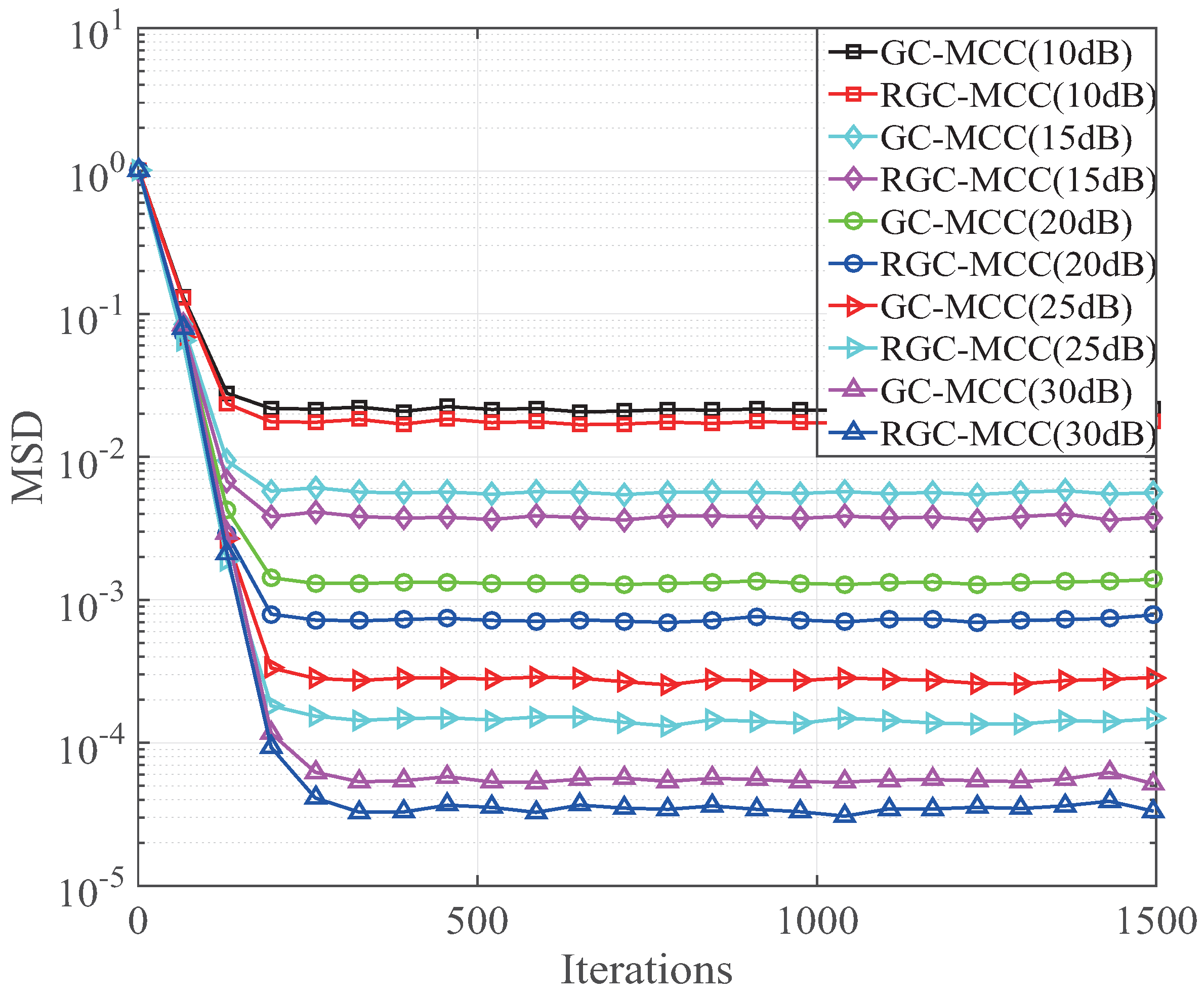
As we know, adaptive filters have been extensively investigated and applied for channel estimation, and have been used in real time systems. Moreover, adaptive filters algorithms have been further developed for sparse channel estimations. Similar to the previous investigations [2,6,7,10,11,12,13,14,15,16,21,22,23,24,26,27], the proposed GC-MCC and RGC-MCC algorithms are investigated and their performance is compared with the SPF-MCC algorithm. In the following experiment, the proposed GC-MCC and RGC-MCC algorithms are investigated in different SNR environments. In this experiment, the step size of the GC-MCC and RGC-MCC algorithms is 0.026, and ${\theta }_{\mathrm{GC}}=3\times {10}^{-4}$ and ${\theta }_{\mathrm{RGC}}=7\times {10}^{-4}$. The MSD performance at different SNRs is shown in Figure 7. It can be seen that the performance of the proposed GC-MCC and RGC-MCC algorithms is improved with the increment of SNR. It is worth noting that the performance of the RGC-MCC is always better than that of the GC-MCC at the same SNR. This is because the reweighting factor provides a selective zero attracting in the RGC-MCC algorithm.

Figure 7. Estimation behavior of the proposed GC-MCC and RGC-MCC algorithms with different SNR.

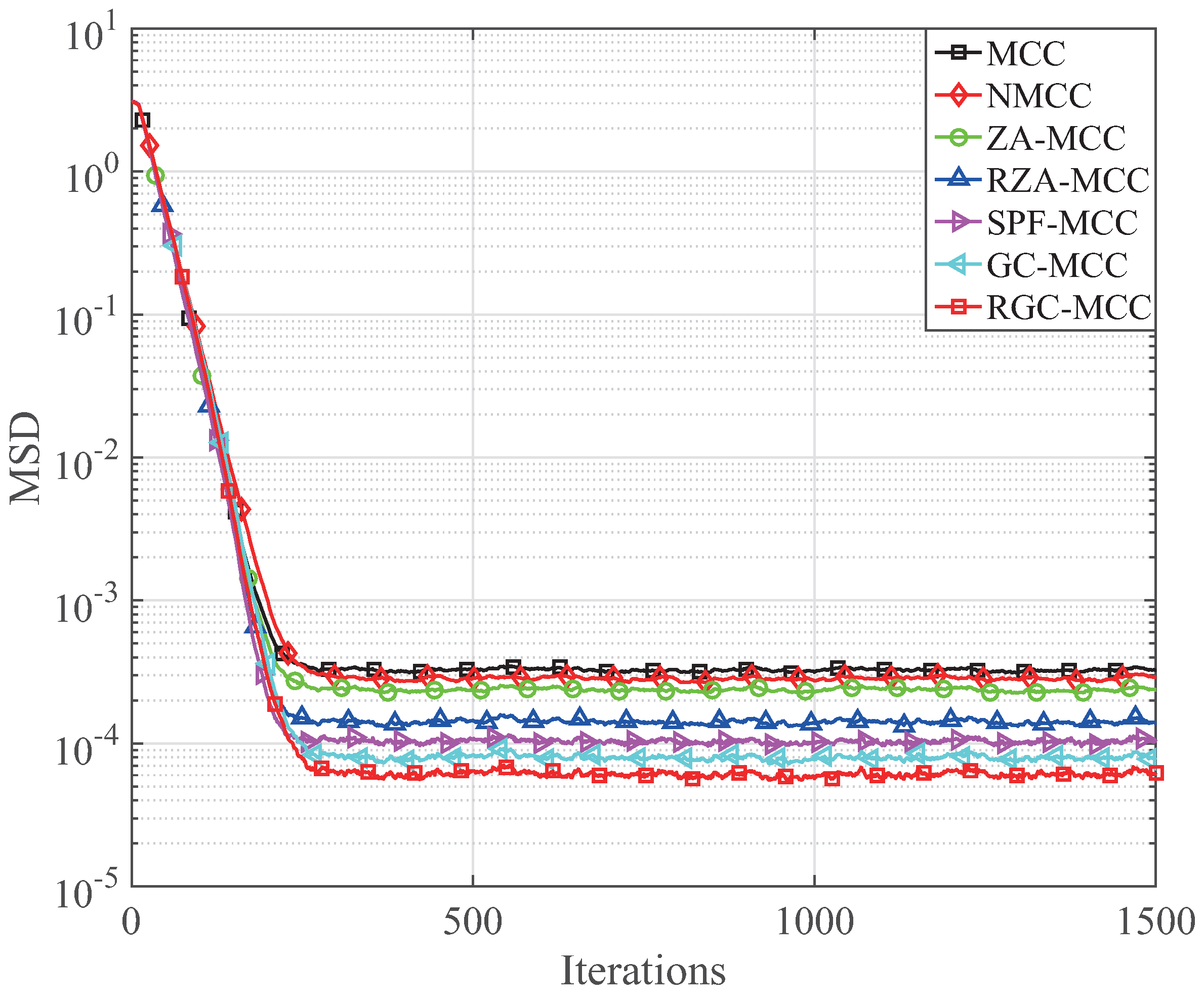
Next, the convergence of the GC-MCC and RGC-MCC algorithms is studied and it is compared with the MCC, NMCC, ZA-MCC, RZA-MCC and SPF-MCC algorithms at SNR = 30 dB. The corresponding simulation parameters for the mentioned algorithms are ${\beta }_{\mathrm{MCC}}=0.0052$, ${\beta }_{\mathrm{NMCC}}=0.085$, ${\beta }_{\mathrm{ZA}}=0.01$, ${\theta }_{\mathrm{ZA}}=3\times {10}^{-5}$, ${\beta }_{\mathrm{RZA}}=0.015$, ${\theta }_{\mathrm{RZA}}=7\times {10}^{-5}$, ${\beta }_{\mathrm{SPF}}=0.016$, ${\theta }_{\mathrm{SPF}}=2.7\times {10}^{-5}$, ${\tau }_1=100$, ${\beta }_{\mathrm{GC}}=0.026$, ${\theta }_{\mathrm{GC}}=3\times {10}^{-4}$, ${\beta }_{\mathrm{RGC}}=0.032$, ${\theta }_{\mathrm{RGC}}=7\times {10}^{-4}$, ${\epsilon }_1=5$ and $\sigma =1000$. Herein, ${\beta }_{\mathrm{NMCC}}$ is the step size of the NMCC algorithm. The convergence of the proposed GC-MCC and RGC-MCC algorithms is given in Figure 8. It can be seen that the convergence of the proposed GC-MCC and RGC-MCC algorithms is better than that of the MCC, NMCC, ZA-MCC, RZA-MCC and SPF-MCC algorithms at the same MSD level. Moreover, our RGC-MCC has the fastest convergence speed rate.

Figure 8. Convergence of the proposed GC-MCC and RGC-MCC algorithms.

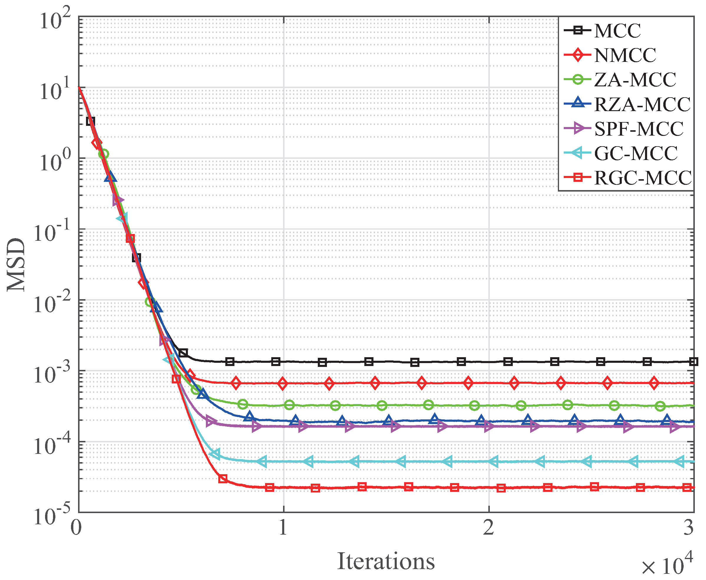
Next, the channel estimation performance of our presented GC-MCC and RGC-MCC algorithms is analyzed under a different sparsity level K that is also the number of the non-zero channel coefficients of the sparse channel. Firstly, only one non-zero channel coefficient is randomly distributed within the unknown sparse channel. This means that the sparsity level is $K=1$. In this experiment, the related parameters are the following ${\beta }_{\mathrm{MCC}}=0.03$, ${\beta }_{\mathrm{NMCC}}=0.4$, ${\beta }_{\mathrm{ZA}}={\beta }_{\mathrm{RZA}}=0.03$, ${\theta }_{\mathrm{ZA}}=8\times {10}^{-5}$, ${\theta }_{\mathrm{RZA}}=2\times {10}^{-4}$, ${\beta }_{\mathrm{SPF}}=0.03$, ${\theta }_{\mathrm{SPF}}=3\times {10}^{-5}$, ${\tau }_1=100$, ${\beta }_{\mathrm{GC}}={\beta }_{\mathrm{RGC}}=0.026$, ${\theta }_{\mathrm{GC}}=3\times {10}^{-4}$, ${\theta }_{\mathrm{RGC}}=7\times {10}^{-4}$ and ${\epsilon }_1=5$. The MSD performance of the GC-MCC and RGC-MCC algorithms is demonstrated in Figure 9 for $K=1$. It can be seen in Figure 9 that the steady-state MSD of our presented GC-MCC and RGC-MCC algorithms is lower than that of the mentioned MCC algorithms with the same convergence speed. The channel estimations with respect to the MSD for $K=3$ and $K=5$ are given in Figure 10 and Figure 11, respectively. When the sparsity level increases from $K=3$ to $K=5$, the MSD floor is increased in comparison with $K=1$ because the sparseness is reduced. However, it is worth noting that our proposed GC-MCC and RGC-MCC algorithms still outperform the existing MCC and its sparse forms. In addition, the RGC-MCC always achieves the lowest MSD for different K.

Figure 9. MSD performance of the proposed GC-MCC and RGC-MCC algorithms for K = 1.

Figure 10. MSD performance of the proposed GC-MCC and RGC-MCC algorithms for K = 3.

Figure 11. MSD performance of the proposed GC-MCC and RGC-MCC algorithms for K = 5.

Then, a realistic IEEE 802.15.4a channel model, which can be downloaded from [39], that works in CM1 mode is employed to discuss the effectiveness of the proposed GC-MCC and RGC-MCC algorithms. The simulation parameters are ${\beta }_{\mathrm{MCC}}=0.002$, ${\beta }_{\mathrm{NMCC}}=0.8$, ${\beta }_{\mathrm{ZA}}=0.0011$, ${\beta }_{\mathrm{RZA}}=0.001$, ${\theta }_{\mathrm{ZA}}=6\times {10}^{-6}$, ${\theta }_{\mathrm{RZA}}=9\times {10}^{-5}$, ${\theta }_{\mathrm{SPF}}=8\times {10}^{-6}$, ${\tau }_1=100$, ${\beta }_{\mathrm{SPF}}={\beta }_{\mathrm{GC}}={\beta }_{\mathrm{RGC}}=0.001$, ${\theta }_{\mathrm{GC}}=5\times {10}^{-4}$, ${\theta }_{\mathrm{RGC}}=3\times {10}^{-4}$ and ${\epsilon }_1=5$. The simulation result is given in Figure 12. It is found that the proposed GC-MCC and RGC-MCC algorithms achieve better performance with respect to the MSD, which means that the proposed GC-MCC and RGC-MCC algorithms have small MSDs.

Figure 12. Estimation behavior of the proposed GC-MCC and RGC-MCC algorithms for estimating a IEEE 802.15.4a channel in CM1 mode.

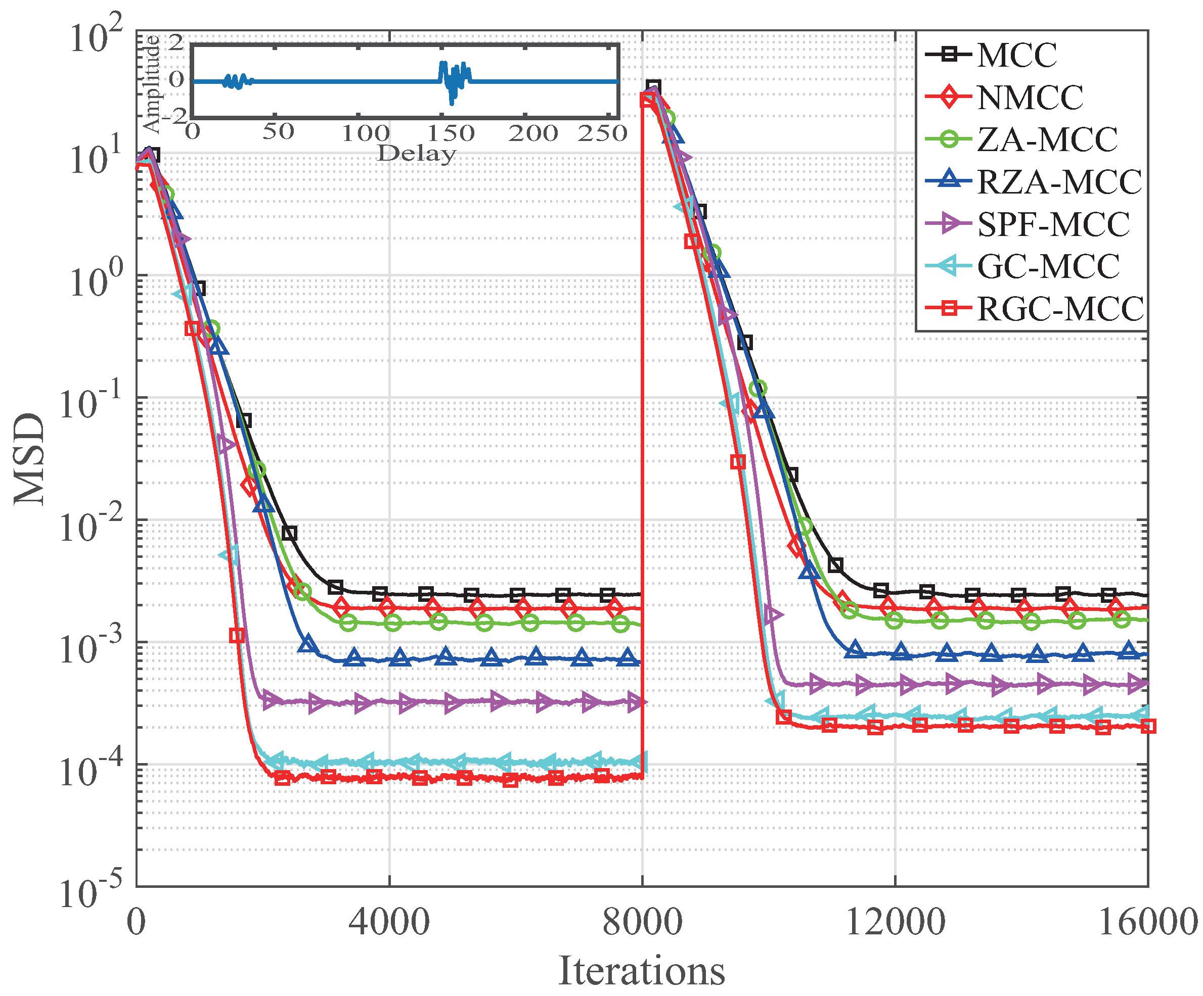
At last, our GC-MCC and RGC-MCC algorithms are used for estimating an echo channel to further discuss their channel estimation performance. The sparseness measurement of the echo channel is defined as ${\vartheta }_{12}=\frac{M}{M-\sqrt{M}}\left(1-{∥\mathbf{g}∥}_1/\phantom{{∥\mathbf{g}∥}_1\sqrt{M}{∥\mathbf{g}∥}_2}\sqrt{M}{∥\mathbf{g}∥}_2\right)$. In this experiment, ${\vartheta }_{12}=0.8222$ and ${\vartheta }_{12}=0.7362$ are used for discussing the estimation performance for the first 8000 iterations and after 8000 iterations, respectively. For the echo channel, its total length is 256 and there are 16 non-zero coefficients in the total echo channel. The simulation parameters are ${\beta }_{\mathrm{MCC}}=0.0055$, ${\beta }_{\mathrm{NMCC}}=1.3$, ${\beta }_{\mathrm{ZA}}={\beta }_{\mathrm{RZA}}=0.0055$, ${\theta }_{\mathrm{ZA}}=4\times {10}^{-6}$, ${\theta }_{\mathrm{RZA}}=1\times {10}^{-5}$, ${\beta }_{\mathrm{SPF}}=0.0055$, ${\theta }_{\mathrm{SPF}}=1\times {10}^{-5}$, ${\tau }_1=5$, ${\beta }_{\mathrm{GC}}=0.0045$, ${\beta }_{\mathrm{RGC}}=0.004$, ${\theta }_{\mathrm{GC}}=3\times {10}^{-5}$, ${\theta }_{\mathrm{RGC}}=3\times {10}^{-5}$ and ${\epsilon }_1=5$. The estimation behavior of the proposed GC-MCC and RGC-MCC algorithms for the echo channel is depicted in Figure 13. From Figure 13, we found that our GC-MCC and RGC-MCC algorithms outperform the MCC, NMCC and spare MCC algorithms with respect to both the steady-state MSD and convergence. Although the sparsity reduces from ${\vartheta }_{12}=0.8222$ to ${\vartheta }_{12}=0.7362$, our GC-MCC and RGC-MCC algorithms are still superior to the other MCC algorithms, which means that our GC-MCC and RGC-MCC algorithms have little effect on the sparsity under the mixture-noised sparse channel.

Figure 13. Estimation behavior of the proposed GC-MCC and RGC-MCC algorithms for an echo channel.

Based on the parameter analysis and performance investigation of our proposed GC-MCC and RGC-MCC algorithms, we can summarize that the proposed RGC-MCC algorithm can provide the fastest convergence speed rate in comparison with all the mentioned algorithms when they converge to the same steady-state MSD level. Also, the proposed RGC-MCC algorithm provides the lowest steady-state MSD when all the MCC algorithms have the same convergence speed rate. In addition, the proposed GC- and PGC-MCC algorithms outperform the MCC, NMCC and the related sparse MCC algorithms. This is because the proposed GC- and RGC-MCC algorithms exert the $l_0$-norm penalty on the large group to seek the non-zero channel coefficients quickly; then, they provide $l_1$-norm constraint on the small group to attract the zero or near-zero channel coefficients to zero quickly. Thus, both the GC- and RGC-MCC can provide a faster convergence and a lower steady-state MSD. However, both the GC- and RGC-MCC increase the computational complexity by calculating the group matrix. Additionally, the complexity of the RGC-MCC algorithm also comes from the computation of the reweighting factor. However, the complexity of the GC-MCC and RGC-MCC algorithms is comparable with the previously reported sparse MCC algorithms. According to the early published articles, we believe that the proposed GC-MCC and RGC-MCC algorithms can be used in a real system.

5. Conclusions

In this paper, a GC-MCC algorithm and a RGC-MCC algorithm have been proposed and they have been derived mathematically in detail. These two algorithms were implemented by exerting a non-uniform norm on the MCC’s cost function, and then, the non-uniform norm was split into $l_0$-norm and $l_1$-norm to give penalties on the large and small groups. The channel estimation behaviors of both the GC-MCC and RGC-MCC algorithms were investigated over a sparse channel and an echo channel under the mixture noise environment. The simulation results from these two channels demonstrated that the proposed GC-MCC and RGC-MCC algorithms can provide faster convergence and smaller MSD for different sparsity levels. Especially, the RGC-MCC algorithm achieves the fastest convergence and smallest MSD.