On the Capacity and the Optimal Sum-Rate of a Class of Dual-Band Interference Channels ^†

Abstract

We study a class of two-transmitter two-receiver dual-band Gaussian interference channels (GIC) which operates over the conventional microwave and the unconventional millimeter-wave (mm-wave) bands. This study is motivated by future 5G networks where additional spectrum in the mm-wave band complements transmission in the incumbent microwave band. The mm-wave band has a key modeling feature: due to severe path loss and relatively small wavelength, a transmitter must employ highly directional antenna arrays to reach its desired receiver. This feature causes the mm-wave channels to become highly directional, and thus can be used by a transmitter to transmit to its designated receiver or the other receiver. We consider two classes of such channels, where the underlying GIC in the microwave band has weak and strong interference, and obtain sufficient channel conditions under which the capacity is characterized. Moreover, we assess the impact of the additional mm-wave band spectrum on the performance, by characterizing the transmit power allocation for the direct and cross channels that maximizes the sum-rate of this dual-band channel. The solution reveals conditions under which different power allocations, such as allocating the power budget only to direct or only to cross channels, or sharing it among them, becomes optimal.

1. Introduction

Current technology such as 4G (e.g., [1]) is rapidly becoming inadequate to support the exponential growth in wireless traffic [2]. Moreover, the potential for improvement of network throughput in 4G is limited due to the shortage of spectrum in the incumbent microwave band (i.e., carrier frequencies below 6 GHz). Thus, methods to tackle the ever growing amount of mobile traffic has become a key research area (see [3] and references therein). Several new technologies are being considered, among which employing additional spectrum in the 28–300 GHz frequency range, often referred to as the millimeter wave (mm-wave) band, seems to be a promising solution to the problem of spectrum scarcity [3,4]. Specifically, integrating additional spectrum from the mm-wave band to complement transmissions in the microwave band is poised to play a central role in the functioning of 5G networks.

Transmission in the mm-wave band is distinctly different from that in the microwave band. Due to higher operating frequencies, omnidirectional transmission in the mm-wave band is subject to much higher absorption and power loss [5] compared to that in the microwave band, and thus a transmitter needs to employ beamforming with highly directional antenna arrays to counter this loss and reach its receiver [2]. However, beamforming constrains most of the transmission energy to the line-of-sight (LOS) component and very few, if any, significant non-LOS components exist [6,7]. Thus, transmission in this band is highly directional and point-to-point. Such mm-wave channels can support high data rates due to their vast bandwidth, but nevertheless are prone to blockage and absorption [8] due to their point-to-point nature. In contrast, microwave links are much more reliable due to rich scattering and diffraction, but cannot support as high rates as the mm-wave links. Thus, in a dual-band setting, conventional traffic and control information can be reliably communicated over microwave links, and high data-rate traffic can be sent through mm-wave links [2,7,9,10,11,12,13,14,15].

Most studies on microwave and mm-wave dual-band transmission have focused on how to improve network layer performance metrics of cellular access or backhaul networks by using the high-bandwidth, highly directional mm-wave links [9,13]. For example, the authors in [7] posed the problem of optimal resource allocation in a cellular setting in the dual microwave and mm-wave band, and showed that certain network level performance parameters, e.g., the number of simultaneously supported users and the link connection probability, are vastly improved with their proposed solution. Similarly, the authors in [11] study a two-tier cellular network where the 60 GHz band is used to create point-to-point directional links, and the 70 GHz band is used to establish long range connections just as the microwave band is used in our work, and propose a hybrid scheme involving both bands that improves the network throughput. In a more related article [14], the authors characterize the benefits of beamforming over a point-to-point dual band multi-antenna channel, and study the performance of a hybrid adaptive queueing scheme over both bands that maximizes the delay-constrained throughput.

Recent works on joint transmission in the microwave band and mm-wave band [14,16,17,18,19,20] indicate that it is possible to isolate the transmissions in the microwave band from that in the mm-wave band, and communicate over the two bands simultaneously. For example, the authors in [14] designed a queue-based scheme that transmits from a single transmitter to a single receiver simultaneously over the 3 GHz microwave band and the 30 GHz mm-wave band using beamforming, and conducted successful practical experiments in this dual-band setup. In addition, Intel has recently announced the production of a dual-band modem that supports both sub-6 GHz and 28 GHz bands [16]. Moreover, recent works on resource allocation in the microwave and mm-wave dual-band setting in [19,20], and their variant in [21], show that simultaneous transmission in both microwave and mm-wave bands are indeed feasible, and are gaining acceptance as an architecture for cellular access in 5G.

We study here the performance of a two-transmitter two-receiver ($2\times 2$) dual-band interference channel from an information theoretic perspective, where a transmitter communicates to its respective receiver over the microwave band and the mm-wave band simultaneously. In the microwave band, each receiver observes the superposition of signals from both transmitters as in a conventional single band Gaussian interference channel (GIC) [22]. However, as the mm-wave channels are considered to be highly directional, a transmitter in this band is well-modeled as being able to transmit towards one intended receiver, while causing negligible to no interference to the other receiver [6]. This raises the question: to which receiver should a transmitter in the mm-wave band transmit? In this $2\times 2$ GIC, the transmitters in the mm-wave band can transmit from: (a) the first transmitter ($T{x}_1$) to the first receiver ($R{x}_1$), and the second transmitter ($T{x}_2$) to the second receiver ($R{x}_2$); (b) $T{x}_1$ to $R{x}_2$, and $T{x}_2$ to $R{x}_1$; (c) $T{x}_1$ and $T{x}_2$ to $R{x}_2$; or (d) $T{x}_1$ and $T{x}_2$ to $R{x}_1$. We focus here on the first two cases where the transmitters in the mm-wave band either transmit (a) from $T{x}_1$ to $R{x}_1$, and from $T{x}_2$ to $R{x}_2$, i.e., in the direct channels; or (b) from $T{x}_1$ to $R{x}_2$, and from $T{x}_2$ to $R{x}_1$, i.e., in the cross channels; or (c) share the spectrum between the two modes. We denote the resulting channels by Direct-Link IC (DLIC), Cross-Link IC (CLIC) and Direct-and-Cross-Link IC (DCLIC), respectively, and study their capacity.

The capacity of the conventional single band GIC [22] has been characterized when it has strong [22] or very strong interference [23]. We know that, under strong interference, encoding the message at each transmitter with independent Gaussian distributed codewords, and decoding both the desired and the interfering messages at each receiver is the optimal strategy [22]. However, if the GIC has weak interference [24], the capacity and the optimal strategy is still unknown in general.

The $2\times 2$ parallel Gaussian IC (PGIC) consists of several orthogonal parallel channels (sub-channels) such that a $2\times 2$ conventional GIC operates in each sub-channel without interfering with that in other sub-channels [25]. The optimal strategies for the PGIC are not known in general; however, its capacity was characterized in [26] when the GIC in each sub-channel has strong interference. In a related study, the capacity of the ergodic fading GIC was characterized in [27] when each fading state has strong interference. In the dual-band GIC considered here, the number of channel uses in the microwave band and the mm-wave band may differ. We model this with a bandwidth mismatch factor (BMF) in the system model. Note that the dual-band GIC considered here is a special case of the ergodic fading GIC in [27] if one identifies each fading state as a different sub-channel. In the special case that the bandwidth mismatch factor between the microwave and mm-wave bands is 1, it is also a special case of the PGIC in [26].

Moreover, the studies in [26,27] show that if every sub-channel (or fading state) has strong interference, the capacity is achieved by encoding jointly over all sub-channels and decoding messages from both transmitters. Encoding independently over each sub-channel of a PGIC is suboptimal in general [28], except for the GIC in the very weak (noisy) interference regime [29]. In fact, joint encoding over all sub-channels generally achieves better rates as it can potentially offset the weak interference in one or more sub-channels if the other sub-channels have strong interference [28].

In this sequel, we study the capacity of the DCLIC and the CLIC. First, we present a useful result that decomposes the capacity of the DCLIC into that of the underlying CLIC and the set of direct channels. This result shows that the capacity of the DCLIC can be established if the capacity of a corresponding CLIC is known. Hence, we focus on the CLIC next. In particular, we consider two specific classes, the strong CLIC and the weak CLIC, where the underlying GIC in the microwave band has strong and weak interference, respectively, and characterize sufficient conditions on the channel parameters under which their capacity is established.

Resource allocation techniques that maximize the sum-rate or throughput of interference channels have been investigated throughly (e.g., see [25,30,31]) as they indicate how to allocate resources in practice. The DCLIC models a basic multiuser network over the microwave and mm-wave dual-band, whose performance is likely to be dominated by the mm-wave channels due to their large bandwidths [9]. Thus, it is useful to understand how to optimize the performance of the DCLIC over the parameters in the mm-wave band. Therefore, we study the power allocation in the direct and cross channels in the mm-wave band that maximizes the sum-rate of the DCLIC. We derive the optimal powers in closed form, and study how the channel parameters influence the optimal power allocation.

The contributions of this paper are summarized as follows:

• We show that the capacity region of the DCLIC can be decomposed into the capacity region of the underlying CLIC and two non-interfering direct links in the mm-wave band. This illustrates that the cross channels are actively involved in characterizing the capacity of the CLIC, whereas the direct channels improve the rates of individual users.
• We characterize the capacity of the strong CLIC, and observe that the strong interference condition in the microwave band is sufficient to characterize the capacity.
• For the weak CLIC, we characterize sufficient channel conditions under which its capacity is established. This shows that even if the GIC in the microwave band has weak interference, adequately strong cross channels in the mm-wave band are sufficient to characterize the capacity.
• We characterize the optimal power allocation in the direct and cross channels that maximizes the sum-rate of the DCLIC, and study channel conditions under which the optimal power allocation either assigns the entire power budget to a specific subset of channels, or shares the power budget among all channels. We establish a direct relation between the channel parameters and the optimal powers, from which we observe the following:

  -

  The optimal power allocation distributes the power budget among the direct and cross channels following two properties: a waterfilling-like property and a max-min property.

  -

  When the power budget is sufficiently small, the optimal allocation assigns power to either both direct channels, or both cross channels and at most one direct channel.

  -

  Due to the max-min property, the optimal allocation imposes a maximum limit on the cross-channel powers. When the power budget exceeds a certain threshold, the limit on the cross-channel powers are reached, and all additional increments to the power budget are then added only to the direct channels that do not have such limits.

  -

  If the underlying GIC in the microwave band has very strong interference, the optimal power allocation assigns the power budget entirely to the direct channels.

  -

  If the channel parameters satisfy one of the following criteria, then transmitting only in the direct channels is approximately optimal, in the sense that the difference between the sum-rates resulting from allocating to only direct channels and allocating optimally in all channels, is negligibly small: (a) the transmit powers in the underlying GIC in the microwave band is very small; or (b) the cross channel gains in the mm-wave band are very large.

The rest of the paper is organized as follows. We define the system model in Section 2. We present the decomposition result on the DCLIC and the capacity of the strong CLIC in Section 3. We present the capacity result on the weak CLIC in Section 4. In Section 5, we formulate the optimum sum-rate problem and discuss its solution, and we conclude in Section 6.

Notation: We denote sets in calligraphic (e.g., ${\mathcal{A}}_k$), except the sets of reals, positive reals, and positive integers, which are denoted by $\mathbb{R}$, ${\mathbb{R}}_{+}$ and ${\mathbb{Z}}_{+}$, respectively. Vectors are in bold (e.g., $\mathbf{x}$), and $\mathbf{x}⪰\mathbf{0}$ denotes that each element of $\mathbf{x}$ is in ${\mathbb{R}}_{+}$, where $\mathbf{0}$ is the zero vector. We denote by $\mathbb{E}(Y)$ the statistical expectation of a random variable (RV) Y, and by $X\sim \mathcal{N}(\mu ,{\sigma }^2)$ an RV following the Gaussian distribution with mean $\mu$ and variance ${\sigma }^2$. We also denote an n-length vector $(X_1,X_2,\dots ,X_n)$ by $X^n$, the empty set by ∅, ${log}_{2}x$ by $logx$, and define $\mathsf{C}(x):=\frac{1}{2}log(1+x)$.

2. System Model

First, we define the discrete memoryless (DM) model of the DCLIC, and from that we define the Gaussian models. In the DCLIC, a bandwidth mismatch between the first (microwave) band and the second (mm-wave) band may exist. Thus, we assume that during n accesses of the first band, the second band is accessed $n_1(n)$ times as cross channels, and $n_2(n)$ times as direct channels. We model this by two bandwidth mismatch factors (BMF) ${\alpha }_k:={lim}_{n\to \infty }{n}_k(n)/n,k=1,2$. Thus, the total normalized channel uses in the second band is asymptotically $\alpha :={\alpha }_1+{\alpha }_2$, which is shared between the cross channels (${\alpha }_1$) and direct channels (${\alpha }_2$). For ease of exposition, we denote $n_k(n)$ by $n_k$, $k=1,2.$

The $2\times 2$ DM interference channel is defined by $({({\mathcal{X}}_k,{\mathcal{Y}}_k)}_{k=1}^2,p(y_1,y_2|x_1,x_2))$ where ${\mathcal{X}}_k$ and ${\mathcal{Y}}_k$ are the discrete input and output alphabets of user k, $k=1,2,$ and $p(y_1,y_2|x_1,x_2)$ is the set of channel transition probabilities [32] (Chapter 6.1). We define the $2\times 2$ DM DCLIC similarly by the tuple, $({({\mathcal{X}}_k,{\widehat{\mathcal{X}}}_k,{\overline{\mathcal{X}}}_k,{\mathcal{Y}}_k,{\widehat{\mathcal{Y}}}_k,{\overline{\mathcal{Y}}}_k)}_{k=1}^2,p)$, where ${\mathcal{X}}_k$ and ${\mathcal{Y}}_k$ are the input and output alphabets of the interference channel in the first band, ${\overline{\mathcal{X}}}_k$ and ${\overline{\mathcal{Y}}}_k$ are the input and output alphabets for the $T{x}_k$ to $R{x}_k$ direct channels in the second band, $k=1,2,$ and ${\widehat{\mathcal{X}}}_1$ and ${\widehat{\mathcal{Y}}}_2$ (respectively ${\widehat{\mathcal{X}}}_2$ and ${\widehat{\mathcal{Y}}}_1$) are the input and output alphabets for the $T{x}_1$ to $R{x}_2$ (resp. $T{x}_2$ to $R{x}_1$) cross channel in the second band. The joint probability mass function (pmf) of the DCLIC decomposes as

$$\begin{array}{c}p(x_1^n,{\widehat{x}}_1^{n_1},{\overline{x}}_1^{n_2})p(x_2^n,{\widehat{x}}_2^{n_1},{\overline{x}}_2^{n_2})\prod _{\ell =1}^{n}p(y_{1\ell },y_{2\ell }|x_{1\ell },x_{2\ell })\prod _{\ell =1}^{n_1}p({\widehat{y}}_{1\ell }|{\widehat{x}}_{2\ell })p({\widehat{y}}_{2\ell }|{\widehat{x}}_{1\ell })\prod _{\ell =1}^{n_2}p({\overline{y}}_{1\ell }|{\overline{x}}_{1\ell })p({\overline{y}}_{2\ell }|{\overline{x}}_{2\ell }).\hfill \end{array}$$

We define a $(2^{n{R}_1},2^{n{R}_2},n,n_1,n_2)$ code for the DCLIC to consist of (a) two uniformly distributed and independent message sets, ${\mathcal{M}}_1:=\{1,\dots ,2^{n{R}_1}\}$ and ${\mathcal{M}}_2:=\{1,\dots ,2^{n{R}_2}\}$, respectively, for $T{x}_1$ and $T{x}_2$; (b) two encoding functions, ${\varphi }_1$ and ${\varphi }_2$, respectively for $T{x}_1$ and $T{x}_2$ such that ${\varphi }_k:{\mathcal{M}}_k\to {\mathcal{X}}_k^n\times {\widehat{\mathcal{X}}}_k^{n_1}\times {\overline{\mathcal{X}}}_k^{n_2},k=1,2$; and (c) two decoding functions, ${\psi }_1$ and ${\psi }_2$, respectively, for $R{x}_1$ and $R{x}_2$ such that ${\psi }_k:{\mathcal{Y}}_k^n\times {\widehat{\mathcal{Y}}}_k^{n_1}\times {\overline{\mathcal{Y}}}_k^{n_2}\to {\mathcal{M}}_k,k=1,2$.

We define the decoding probability of error at $R{x}_k$ by $P_{e,k}^n:=\mathrm{Pr}\left({\psi }_k(Y_k^n,{\widehat{Y}}_k^{n_1},{\overline{Y}}_k^{n_2})\ne M_k\right),k=1,2.$ We say that $(R_1,R_2)$ is an achievable rate pair of the DCLIC, if there exists a sequence of $(2^{n{R}_1},2^{n{R}_2},n,n_1,n_2)$ codes such that $n_k\le {\alpha }_{k}n,$ and $P_{e,k}^n\to 0$ as $n,n_k\to \infty$ for $k=1,2$. The capacity region of the DCLIC is defined as the closure of the set of all achievable rate tuples.

Following the above notations, the GIC in the first band of the Gaussian DCLIC is modeled as in [22]. The signals received at $R{x}_1$ and $R{x}_2$ are given by

$$\begin{array}{c}{Y}_{1\ell }=X_{1\ell }+a_{21}{X}_{2\ell }+Z_{1\ell },\hfill \end{array}$$

(1)

$$\begin{array}{c}{Y}_{2\ell }=X_{2\ell }+a_{12}{X}_{1\ell }+Z_{2\ell },\ell =1,\dots ,n,\hfill \end{array}$$

(2)

where $X_{k\ell },Y_{k\ell }\in \mathbb{R}$, $a_{km}\in \mathbb{R}$ are coefficients of the channels from $T{x}_k$ to $R{x}_m$, $k\ne m\in \{1,2\}$ ($a_{kk}^2$ are normalized to 1 as in [22]), and $Z_{k\ell }\sim \mathcal{N}(0,1)$ are i.i.d. noise, $k=1,2$. In addition, the codewords now satisfy the average power constraint, $\frac{1}{n}{\sum }_{\ell =1}^n{X}_{k\ell }^2\le Q_k,k=1,2$. The cross links in the second band of the DCLIC are point-to-point, and are modeled as

$$\begin{array}{c}{\widehat{Y}}_{2\ell }=c_{12}{\widehat{X}}_{1\ell }+{\widehat{Z}}_{2\ell },\hfill \end{array}$$

(3)

$$\begin{array}{c}{\widehat{Y}}_{1\ell }=c_{21}{\widehat{X}}_{2\ell }+{\widehat{Z}}_{1\ell },\ell =1,\dots ,n_1,\hfill \end{array}$$

(4)

where ${\widehat{X}}_{k\ell },{\widehat{Y}}_{k\ell }\in \mathbb{R}$, $c_{km}\in \mathbb{R}$ are coefficients of the channels from $T{x}_k$ to $R{x}_m$, $k\ne m\in \{1,2\}$, and ${\widehat{Z}}_{k\ell }\sim \mathcal{N}(0,1)$ are i.i.d. noise. The codewords satisfy the average power constraint, $\frac{1}{n_1}{\sum }_{\ell =1}^{n_1}{\widehat{X}}_{k\ell }^2\le {\widehat{P}}_k,k=1,2.$ The direct links in the second band are similarly modeled as

$$\begin{array}{c}{\overline{Y}}_{1\ell }=d_1{\overline{X}}_{1\ell }+{\overline{Z}}_{1\ell },\hfill \end{array}$$

(5)

$$\begin{array}{c}{\overline{Y}}_{2\ell }=d_2{\overline{X}}_{2\ell }+{\overline{Z}}_{2\ell },\ell =1,\dots ,n_2,\hfill \end{array}$$

(6)

where ${\overline{X}}_{k\ell },{\overline{Y}}_{k\ell }\in \mathbb{R}$, $d_k\in \mathbb{R}$ are the direct channel coefficients, ${\overline{Z}}_{k\ell }\sim \mathcal{N}(0,1)$ are i.i.d. noise, $k=1,2$, and the codewords satisfy the average power constraint, $\frac{1}{n_2}{\sum }_{\ell =1}^{n_2}{\overline{X}}_{k\ell }^2\le {\overline{P}}_k,k=1,2,$ as well. We present the Gaussian DCLIC in Figure 1. We define a $(2^{n{R}_1},2^{n{R}_2},n,n_1,n_2)$ code for the Gaussian DCLIC from that of the DM DCLIC, by choosing all input and output variables to be in $\mathbb{R}$, and by imposing the average power constraints on the codewords, $X_k^n$, ${\widehat{X}}_k^{n_1}$ and ${\overline{X}}_k^{n_2},k=1,2$, defined above.

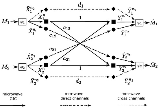
Figure 1. System model of the Gaussian DCLIC, which consists of an underlying GIC in the microwave band and the set of direct channels and cross channels in the mm-wave band.

Next, the Gaussian CLIC is defined from the Gaussian DCLIC by imposing the restrictions, $n_2=0$ and ${\overline{\mathcal{X}}}_k={\overline{\mathcal{Y}}}_k=\varnothing ,k=1,2$, such that the channel outputs in the CLIC are described by (1)–(4), respectively. A $(2^{n{R}_1},2^{n{R}_2},n,n_1)$ code for CLIC is defined from a $(2^{n{R}_1},2^{n{R}_2},n,n_1,n_2)$ code of the Gaussian DCLIC with the above-mentioned restrictions.

For ease of exposition, we define two classes of the CLICs: we say that a CLIC is a strong CLIC or a weak CLIC, if the underlying GIC in the first band has strong interference (i.e., $a_{12}^2\ge 1$, $a_{21}^2\ge 1$) or weak interference (i.e., $a_{12}^2<1$, $a_{21}^2<1),$ respectively. Moreover, a symmetric CLIC is a CLIC where $a^2:=a_{12}^2=a_{21}^2$, $c^2:=c_{12}^2=c_{21}^2$, $Q_1=Q_2$, and ${\widehat{P}}_1={\widehat{P}}_2$. In addition, a symmetric DCLIC is a DCLIC with an underlying symmetric CLIC, and $d^2=d_1^2=d_2^2,{\overline{P}}_1={\overline{P}}_2$.

Finally, the Gaussian model for the DLIC are defined from that of the DCLIC by imposing the restrictions, $n_1=0$ and ${\widehat{\mathcal{X}}}_k={\widehat{\mathcal{Y}}}_k=\varnothing ,k=1,2$, and thus the channel outputs are described by (1), (2), (5) and (6), respectively. In the sequel, we focus on the Gaussian model of the DCLIC and the CLIC.

3. Decomposition Result on the Capacity of the DCLIC

Recall that, in the DCLIC, there are n channel uses in the first band, $n_1$ cross channel uses in the second band, and $n_2$ direct channels uses in the second band. We show below that the capacity of the DCLIC can be decomposed into the capacity of the underlying CLIC, complemented by the direct channels that are used to transmit individual user information to their respective receivers.

Theorem 1.

The capacity region of the DCLIC with BMFs ${\alpha }_1$ and ${\alpha }_2$ is given by the set of all nonnegative rate tuples $(R_1,R_2)$ that satisfy the decomposition

$$\begin{array}{c}{R}_1=r_1+{\alpha }_2\mathsf{C}(d_1^2{\overline{P}}_1),R_2=r_2+{\alpha }_2\mathsf{C}(d_2^2{\overline{P}}_2),\hfill \end{array}$$

(7)

where $(r_1,r_2)$ is an achievable rate tuple in the underlying CLIC with BMF ${\alpha }_1$.

Proof. 

The proof is relegated to Appendix A. ☐

Therefore, an achievable rate pair in the DCLIC with BMFs ${\alpha }_1$ and ${\alpha }_2$ consists of a rate pair achievable in the CLIC with BMF ${\alpha }_1$, and the rate pair achieved in the direct channels, $({\alpha }_2\mathsf{C}(d_1^2{\overline{P}}_1),{\alpha }_2\mathsf{C}(d_2^2{\overline{P}}_2))$. The capacity of the DCLIC can thus be characterized from that of the underlying CLIC. Hence, we focus on the CLIC next. In particular, we consider two specific classes of the CLIC, the strong CLIC and the weak CLIC. First, we present the capacity of the strong CLIC.

Lemma 1.

The capacity region of the strong CLIC with BMF ${\alpha }_1$ is given by the set of all nonnegative rate tuples ($R_1,R_2$) that satisfy

$$\begin{array}{c}{R}_1\le \mathsf{C}(Q_1),\hfill \end{array}$$

(8)

$$\begin{array}{c}{R}_2\le \mathsf{C}(Q_2),\hfill \end{array}$$

(9)

$$\begin{array}{c}{R}_1+R_2\le \mathsf{C}(Q_1+a_{21}^2{Q}_2)+{\alpha }_1\mathsf{C}(c_{21}^2{\widehat{P}}_2),\hfill \end{array}$$

(10)

$$\begin{array}{c}{R}_1+R_2\le \mathsf{C}(Q_2+a_{12}^2{Q}_1)+{\alpha }_1\mathsf{C}(c_{12}^2{\widehat{P}}_1).\hfill \end{array}$$

(11)

The proof of Lemma 1 follows from that of [27] in a straightforward manner. Hence, we omit the proof here, and discuss only the key idea. In the strong CLIC, the GIC in the first band has strong interference. Additionally, in the second band, the cross-channel gains are positive and the direct-channel gains are zero, which results in a GIC with strong interference. Hence, the strong CLIC is a parallel GIC with strong interference in both bands. The capacity is thus achieved by encoding jointly over both bands and decoding messages from both transmitters as in [27].

Moreover, the capacity of the DCLIC with strong underlying CLIC, which follows from Theorem 1 and Lemma 1, is characterized below.

Corollary 1.

The capacity region of the DCLIC with BMFs ${\alpha }_1$ and ${\alpha }_2$ that has a strong underlying CLIC is given by the set of all nonnegative rate tuples ($R_1,R_2$) that satisfy

$$\begin{array}{c}{R}_1\le \mathsf{C}(Q_1)+{\alpha }_2\mathsf{C}(d_1^2{\overline{P}}_1),\hfill \end{array}$$

(12)

$$\begin{array}{c}{R}_2\le \mathsf{C}(Q_2)+{\alpha }_2\mathsf{C}(d_2^2{\overline{P}}_2),\hfill \end{array}$$

(13)

$$\begin{array}{c}{R}_1+R_2\le \mathsf{C}(Q_1+a_{21}^2{Q}_2)+{\alpha }_1\mathsf{C}(c_{21}^2{\widehat{P}}_2)+{\alpha }_2\mathsf{C}(d_1^2{\overline{P}}_1)+{\alpha }_2\mathsf{C}(d_2^2{\overline{P}}_2),\hfill \end{array}$$

(14)

$$\begin{array}{c}{R}_1+R_2\le \mathsf{C}(Q_2+a_{12}^2{Q}_1)+{\alpha }_1\mathsf{C}(c_{12}^2{\widehat{P}}_1)+{\alpha }_2\mathsf{C}(d_1^2{\overline{P}}_1)+{\alpha }_2\mathsf{C}(d_2^2{\overline{P}}_2).\hfill \end{array}$$

(15)

Furthermore, if the DLIC, where the second band is used as direct channels only, has strong underlying GIC, the capacity region follows from Corollary 1 with ${\alpha }_1=0$ and ${\alpha }_2=\alpha$.

4. Capacity of the Weak CLIC

Now, consider the weak CLIC where the underlying GIC has weak interference. Recall that in a conventional GIC with weak interference, decoding both messages is suboptimal in general. However, in the weak CLIC, if messages are encoded jointly over both bands and the cross channels in the second band are sufficiently strong, then decoding both messages is indeed optimal. We characterize the sufficient conditions below.

Lemma 2.

Provided the channel parameters of the CLIC with BMF ${\alpha }_1$ satisfy $a_{12}^2<1$, $a_{21}^2<1$, as well as the conditions

$$\begin{array}{c}(1+Q_1)(1+Q_2)\le (1+a_{12}^2{Q}_1){(1+c_{12}^2{\widehat{P}}_1)}^{{\alpha }_1},\hfill \end{array}$$

(16)

$$\begin{array}{c}(1+Q_1)(1+Q_2)\le (1+a_{21}^2{Q}_2){(1+c_{21}^2{\widehat{P}}_2)}^{{\alpha }_1},\hfill \end{array}$$

(17)

the following inequalities hold

$$\begin{array}{c}I(X_1^n;Y_1^n|X_2^n)\le I(X_1^n;Y_2^n)+n{\alpha }_1\mathsf{C}(c_{12}^2{\widehat{P}}_1),\hfill \end{array}$$

(18)

$$\begin{array}{c}I(X_2^n;Y_2^n|X_1^n)\le I(X_2^n;Y_1^n)+n{\alpha }_1\mathsf{C}(c_{21}^2{\widehat{P}}_2),\hfill \end{array}$$

(19)

for all $X_1^n$ and $X_2^n$ with product distributions $p(x_1^n)p(x_2^n)$ on ${\mathbb{R}}^n\times {\mathbb{R}}^n,n\in {\mathbb{Z}}_{+}$, which satisfy the average power constraints, $\frac{1}{n}{\sum }_{\ell =1}^n{X}_{k\ell }^2\le Q_k,k=1,2$.

Proof. 

We prove only (18) as (19) follows similarly. From the system model for the first band in (1) and (2), we have

$$\begin{array}{cc}\hfill I(X_1^n;Y_1^n|X_2^n)-I(X_1^n;Y_2^n)& =h(X_1^n+Z_1^n)-h(Z_1^n)-h(X_2^n+a_{12}{X}_1^n+Z_2^n)+h(X_2^n+Z_2^n)\hfill \\ & \stackrel{(a)}{\le }h(X_2^n+Z_2^n)-h(Z_2^n)+h(X_1^n+Z_1^n)-h(a_{12}{X}_1^n+Z_2^n)\hfill \\ & \stackrel{(b)}{=}I(X_2^n;X_2^n+Z_2^n)-\{h(X_1^n+Z_1^n+Z_3^n)-h(X_1^n+Z_1^n)\}-nlog|a_{12}|\hfill \\ & \stackrel{(c)}{\le }n\mathsf{C}(Q_2)-I(Z_3^n;Z_3^n+Z_1^n+X_1^n)-nlog|a_{12}|\hfill \\ & \stackrel{(d)}{=}n\mathsf{C}(Q_2)-\sum _{\ell =1}^n\left(h(Z_{3\ell }|Z_3^{n-\ell })-h(Z_{3\ell }|Z_3^{n-\ell },Z_3^n+Z_1^n+X_1^n)\right)-nlog|a_{12}|\hfill \\ & \stackrel{(e)}{\le }n\mathsf{C}(Q_2)-\sum _{\ell =1}^n\left(h(Z_{3\ell })-h(Z_{3\ell }|Z_{3\ell }+Z_{1\ell }+X_{1\ell })\right)-nlog|a_{12}|\hfill \\ & \stackrel{(f)}{=}n\mathsf{C}(Q_2)-\sum _{\ell =1}^{n}I(Z_3;Z_3+Z_1+X_{1\ell })-nlog|a_{12}|\hfill \\ & \stackrel{(g)}{\le }n\mathsf{C}(Q_2)-\sum _{\ell =1}^{n}I(Z_3;Z_3+Z_1+X_{1\ell }^{*})-nlog|a_{12}|\hfill \\ & \stackrel{(h)}{=}n\mathsf{C}(Q_2)+\sum _{\ell =1}^n\frac{1}{2}log\frac{Q_{1\ell }+1}{Q_{1\ell }+1/a_{12}^2}-nlog|a_{12}|\hfill \\ & \stackrel{(i)}{\le }n\mathsf{C}(Q_2)+\frac{n}{2}log\frac{\frac{1}{n}{\sum }_{\ell =1}^n{Q}_{1\ell }+1}{\frac{1}{n}{\sum }_{\ell =1}^n{Q}_{1\ell }+1/a_{12}^2}-nlog|a_{12}|\hfill \\ & \stackrel{(j)}{\le }\frac{n}{2}log\frac{(1+Q_1)(1+Q_2)}{(1+a_{12}^2{Q}_1)}\hfill \\ & \stackrel{(k)}{\le }\frac{{\alpha }_{1}n}{2}log(1+c_{12}^2{\widehat{P}}_1),\hfill \end{array}$$

where (a) follows from unconditioning, $h(X_2^n+a_{12}{X}_1^n+Z_2^n)\ge h(X_2^n+a_{12}{X}_1^n+Z_2^n|X_2^n)=h(a_{12}{X}_1^n+Z_2^n)$, and since $h(Z_1^n)=h(Z_2^n)$; (b) follows since $1/a_{12}^2>1$, and thus $h(a_{12}{X}_1^n+Z_2^n)=h(a_{12}{X}_1^n+Z_1^n)=h(X_1^n+{Z_1}^n/a_{12})+nlog|a_{12}|=h(X_1^n+Z_3^n+Z_2^n)+nlog|a_{12}|$, where $Z_{3\ell }\sim \mathcal{N}(0,1/a_{12}^2-1)$, are i.i.d.; (c) follows since the first term in b is maximized by $X_{2\ell }\sim \mathcal{N}(0,Q_2)$, i.i.d.; (d) follows from the chain rule; (e) follows since $Z_{3\ell }$ are i.i.d., and since unconditioning does not reduce entropy; (f) follows by replacing the i.i.d. RVs, $Z_{3\ell }$ and $Z_{1\ell }$, with $Z_3\sim \mathcal{N}(0,1/a_{12}^2-1)$ and $Z_1\sim \mathcal{N}(0,1),$ respectively; (g) follows by invoking the worst additive noise result of [33] to every mutual information term inside the summation of (f), where $X_{1\ell }^{*}\sim \mathcal{N}(0,Q_{1\ell })$, with $Q_{1\ell }:=\mathbb{E}(X_{1\ell }^2)$, and $\frac{1}{n}{\sum }_{\ell =1}^n{Q}_{1\ell }\le Q_1$; (h) follows from the differential entropy of Gaussian RVs; (i) follows since the log function is concave in ${\{Q_{1\ell }\}}_{\ell =1}^n$; (j) follows since $\frac{1}{n}{\sum }_{\ell =1}^n{Q}_{1\ell }\le Q_1$; and (k) follows from condition (16). ☐

We characterize the capacity of the weak CLIC under the conditions of Lemma 2 below.

Theorem 2.

The capacity region of the weak CLIC with BMF ${\alpha }_1$ that satisfies the conditions in (16) and (17) is given by the set of all nonnegative rate tuples $(R_1,R_2)$ that satisfy

$$\begin{array}{c}{R}_1\le \mathsf{C}(Q_1),\hfill \end{array}$$

(20)

$$\begin{array}{c}{R}_2\le \mathsf{C}(Q_2),\hfill \end{array}$$

(21)

$$\begin{array}{c}{R}_1+R_2\le \mathsf{C}(Q_1+a_{21}^2{Q}_2)+\alpha \mathsf{C}(c_{21}^2{\widehat{P}}_2),\hfill \end{array}$$

(22)

$$\begin{array}{c}{R}_1+R_2\le \mathsf{C}(Q_2+a_{12}^2{Q}_1)+\alpha \mathsf{C}(c_{12}^2{\widehat{P}}_1).\hfill \end{array}$$

(23)

Proof. 

The proof is relegated to Appendix B. ☐

The result shows that, in the weak CLIC, where sufficient interference forwarding is not possible through the underlying weak GIC, if the cross links in the second band are sufficiently strong, it is possible to forward enough interference by encoding jointly over both bands such that decoding both messages becomes optimal. Hence, these conditions can be classified as being able to push the receivers to the “strong interference regime over both bands”.

Next, we illustrate the relationship between the channel parameters in (16) and (17) with an example of a symmetric weak CLIC, where (16) and (17) imply the same condition. We denote by $c_{\mathsf{min}}^2:=({((1+Q_1)(1+Q_2)/(1+a^2{Q}_1))}^{1/{\alpha }_1}-1)/{\widehat{P}}_1$, and ${\alpha }_{1,\mathsf{min}}:=log((1+Q_1)(1+Q_2)/(1+a^2{Q}_1))/log(1+c^2{\widehat{P}}_1)$, respectively the minimum $c^2$ and the minimum ${\alpha }_1$ required to achieve (16), and show the interplay between $a^2,c_{\mathsf{min}}^2$ and ${\alpha }_{1,\mathsf{min}}$ for $Q_1=Q_2={\widehat{P}}_1=1$.

In Figure 2a, we plot $c_{\mathsf{min}}^2$ against $a^2\in (0,1)$ for ${\alpha }_1\in \{0.5,1,2\}$. Note that $c_{\mathsf{min}}^2$ reduces monotonically as $a^2$ or ${\alpha }_1$ increases. This follows since, if $a^2$ increases, then the first band forwards more interference, and, if ${\alpha }_1$ increases, then the pre-log factor of the cross-channel capacity increases. In either case, smaller $c_{\mathsf{min}}^2$ is required to achieve (16). Similarly in Figure 2b, we plot ${\alpha }_{1,\mathsf{min}}$ against $a^2\in (0,1)$ for $c^2\in \{0.5,1,2\}$, and note that ${\alpha }_{1,\mathsf{min}}$ reduces as $a^2$ or $c^2$ increases. Finally, in Figure 2c, we depict the set of cross-channel gains ($a^2$ and $c^2$) of a symmetric CLIC with $Q_1=Q_2={\widehat{P}}_1=1,{\alpha }_1=2$, and partition it depending on whether the capacity has been characterized in each set. Note that the capacity for the set where $a^2<1$ and $c^2<c_m^2$ has not been characterized yet.

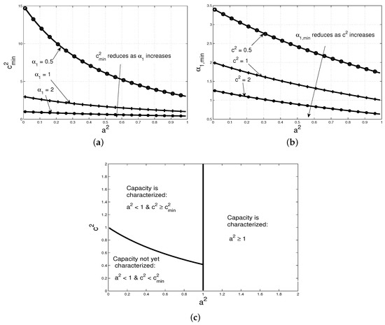
Figure 2. In (a,b), we plot $c_{\mathsf{min}}^2$ and ${\alpha }_{1,\mathsf{min}}$, respectively. In (c), the channel gains of a symmetric CLIC is partitioned based on whether its capacity has been characterized in each set.

5. The Optimal Sum-Rate Problem

In this section, we study the power allocation scheme over the direct and cross channels in the DCLIC that maximizes its sum-rate. Recall from Corollary 1 that, if the underlying GIC of the DCLIC has strong interference (i.e., $a_{12}^2\ge 1$ and $a_{21}^2\ge 1$), then the sum-rate of the DCLIC is known for all values of the remaining channel parameters, and, in particular, for all transmit powers in the second band. Therefore, we pose this problem for the class of DCLICs with strong underlying GIC (see [A1] below). Also recall that the normalized bandwidth ($\alpha$) of the second band is shared between the direct channels (${\alpha }_2$) and the cross channels (${\alpha }_1$). We denote the fraction of $\alpha$ alloted to the direct and cross channels by $\beta$ and $\overline{\beta }$, respectively, where $\beta :={\alpha }_2/\alpha$ and $\overline{\beta }:=1-\beta ={\alpha }_1/\alpha$, and $\beta ,\overline{\beta }\in (0,1)$. Thus, $\beta$ provides a trade-off between the bandwidths in the direct channels ($\beta \alpha$) and the cross channels ($\overline{\beta }\alpha$).

We formulate the problem under the following assumptions:

• the underlying GIC of the DCLIC has strong interference, but not very strong interference, $1\le a_{12}^2<1+Q_1$ and $1\le a_{21}^2<1+Q_2$;
• the underlying GIC of the DCLIC satisfies: $Q_2+a_{12}^2{Q}_1=Q_1+a_{21}^2{Q}_2$;
• $\beta$ and $\overline{\beta }$ are fixed a priori;
• the transmission power in the direct channel ($p_k$) and cross channel ($q_k$) from transmitter k ($T{x}_k$) satisfy the constraint, $\beta p_k+\overline{\beta }{q}_k=P,k=1,2$, where P is the power budget.

In [A1], we assume that the underlying GIC does not have very strong interference, since the power allocation in that case is trivial (see Section 5.4). For ease of exposition, we assume in [A2] that the underlying GIC receives equal power in both its receivers. Note that the class of GICs that satisfies [A2] also contains the symmetric GICs. Moreover, the analysis under [A2] reveals enough insight such that it can be extended to the general case (see Remark 1).

In [A3], $\beta$ is assumed to be fixed a priori and known. This models practical constraints in many wireless networks where dynamically allocating the bandwidth may not be feasible or straightforward [34]. In [A4], we assume that power budget (P) in both transmitters are the same. There is no loss of generality in this assumption as the relative difference between the power budgets of the first and the second user can be absorbed into the channel gains.

5.1. Problem Formulation and Solution

For a fixed power allocation $(p_1,q_1,p_2,q_2)$ in the mm-wave channels, we denote the sum-rate achievable at $R{x}_1$ and $R{x}_2$ in (14) and (15) by ${\Sigma }_1$ and ${\Sigma }_2$, and the interference-free sum-rate given by the sum of individual rates in (12) and (13) by $\Sigma$, and present them below

$$\begin{array}{c}{\Sigma }_1:=A_1+\frac{\alpha \overline{\beta }}{2}log(1+c_{21}^2{q}_2)+\frac{\alpha \beta }{2}\left(log(1+d_1^2{p}_1)+log(1+d_2^2{p}_2)\right),\hfill \end{array}$$

(24)

$$\begin{array}{c}{\Sigma }_2:=A_2+\frac{\alpha \overline{\beta }}{2}log(1+c_{12}^2{q}_1)+\frac{\alpha \beta }{2}\left(log(1+d_1^2{p}_1)+log(1+d_2^2{p}_2)\right),\hfill \end{array}$$

(25)

$$\begin{array}{c}\Sigma :=A+\frac{\alpha \beta }{2}\left(log(1+d_1^2{p}_1)+log(1+d_2^2{p}_2)\right),\hfill \end{array}$$

(26)

where $A_1:=\frac{1}{2}log(1+Q_1+a_{21}^2{Q}_2),A_2:=\frac{1}{2}log(1+Q_2+a_{12}^2{Q}_1)$ and $A:=\frac{1}{2}log(1+Q_1)(1+Q_2)$. Furthermore, they satisfy $A_1=A_2<A$ due to [A2] and [A1]. Therefore, a necessary and sufficient condition for R to be an achievable sum-rate of the DCLIC is $R\le min\{{\Sigma }_1,{\Sigma }_2,\Sigma \}$, for some power allocation ($p_1,q_1,p_2,q_2$). The optimization problem that maximizes R over the transmit powers ($p_1,q_1,p_2,q_2$) is then

$$\begin{array}{cc}\hfill \left[\mathbf{P}\mathbf{1}\right]\mathrm{maximize}& R\hfill \end{array}$$

$$\begin{array}{cc}\hfill \mathrm{subject}\mathrm{to}\text{:}& R\le {\Sigma }_1,\hfill \end{array}$$

(27)

$$\begin{array}{c}R\le {\Sigma }_2,\hfill \end{array}$$

(28)

$$\begin{array}{c}R\le \Sigma ,\hfill \end{array}$$

(29)

$$\begin{array}{c}\beta p_1+\overline{\beta }{q}_1=P,\hfill \end{array}$$

(30)

$$\begin{array}{c}\beta p_2+\overline{\beta }{q}_2=P,\hfill \end{array}$$

(31)

$$\begin{array}{c}(p_1,q_1,p_2,q_2,R)⪰\mathbf{0}.\hfill \end{array}$$

(32)

Note that $\left[\mathbf{P}\mathbf{1}\right]$ is a convex optimization problem, since its objective function R is linear, the equality constraints (30) and (31) are affine, and the inequality constraints (27)–(29) are convex. Furthermore, $\left[\mathbf{P}\mathbf{1}\right]$ satisfies Slater’s condition [35] (Chapter 5.2.3), and thus it can be solved using the Karush–Kuhn–Tucker (KKT) conditions [35] (Chapter 5.5.3). We relegate the details to Appendix C.

It is well known that optimal power allocation in parallel Gaussian point-to-point channels follows the Waterfilling (WF) property. Due to this, if the power budget is sufficient small, it is allocated entirely to the “strongest” sub-channel, and, as the power budget is increased, power is allocated to the other “weaker” sub-channels, in addition to the strongest one (see Chapter 3.4.3 in [32]). In the ensuing discussion, it becomes clear that the optimal power allocation in $\left[\mathbf{P}\mathbf{1}\right]$ (hereby referred to as “the optimal allocation”) has two noticeable properties: a WF-like property, due to which it assigns power to the cross and direct channels following a WF-like allocation, and a max-min property, due to which it increases the minimum of the sum-rate constraints.

Due to its WF-like property, the optimal allocation assigns the entire power budget (P) to only a subset of all the direct and cross channels, depending on channel conditions that indicate whether the direct channels are stronger than the cross channels or vice versa. Moreover, if P is sufficiently increased, it becomes optimal to allocate power to the remaining set of channels. In addition, since the objective of the problem is to maximize $min\{{\Sigma }_1,{\Sigma }_2,\Sigma \}$, the optimal allocation assigns powers in such a way that minimizes or eliminates any difference between ${\Sigma }_1,{\Sigma }_2$ and $\Sigma$. We observe that, due to this property (max-min property), the optimal allocation imposes a maximum limit on the cross-channel powers, which is unlike WF in [32] where no such limit exists.

We study the optimal allocation by partitioning the entire set of channel parameters and P into disjoint sets (${\mathcal{S}}_{(.)}$), such that the optimal allocation can be classified according to the power levels in the direct and cross channels in each set. Without loss of generality, we present the optimal allocation under $c_{21}^2>c_{12}^2$ in Table 1, and study it in detail. In this case, only fours sets, ${\mathcal{S}}_D$, ${\mathcal{S}}_C$, ${\mathcal{S}}_{CD}$ and ${\mathcal{S}}_{\mathsf{sat}}$, are sufficient. The power allocation under $c_{21}^2<c_{12}^2$ can be readily obtained from Table 1 by swapping the indices 1 and 2, and the case with $c_{21}^2=c_{12}^2$ is briefly discussed in Section 5.3.

Table 1. Optimal power allocation and conditions of sets in ${\mathbf{OA}}_{\mathbf{1}}.$

Set		Optimal Powers			Condition
${\mathcal{S}}_D$	$p_1={\displaystyle \frac{P}{\beta }},$	$q_1=0,$	$p_2={\displaystyle \frac{P}{\beta }},$	$q_2=0,$	$g_1(P)>1$
${\mathcal{S}}_C$	$p_1=0,$	$q_1={\displaystyle \frac{P}{\overline{\beta }}},$	$p_2={\displaystyle \frac{P(c_{21}^2-c_{12}^2)}{\beta c_{21}^2}},$	$q_2={\displaystyle \frac{c_{12}^2}{c_{21}^2}}{\displaystyle \frac{P}{\overline{\beta }}},$	$P<P_4^{*},g_2(P)<1$
${\mathcal{S}}_{\mathsf{sat}}$	$p_1={\displaystyle \frac{P}{\beta }}-{\displaystyle \frac{\overline{\beta }(\gamma -1)}{\beta c_{12}^2}},$	$q_1={\displaystyle \frac{\gamma -1}{c_{12}^2}},$	$p_2={\displaystyle \frac{P}{\beta }}-{\displaystyle \frac{\overline{\beta }(\gamma -1)}{\beta c_{21}^2}},$	$q_2={\displaystyle \frac{\gamma -1}{c_{21}^2}},$	$P\ge P_4^{*},g_3(P)<1$
${\mathcal{S}}_{CD}$	$p_1={\displaystyle \frac{P-\overline{\beta }{q}_1}{\beta }},$	$q_1={\displaystyle \frac{F(P)}{c_{12}^2}},$	$p_2={\displaystyle \frac{P-\overline{\beta }{q}_2}{\beta }},$	$q_2={\displaystyle \frac{c_{12}^2}{c_{21}^2}}{q}_1,$	complement of other conditions

For notational convenience, we express the optimal powers and the conditions of the sets ${\mathcal{S}}_{(.)}$ in Table 1 in terms of the following functions:

$$\begin{array}{c}{g}_1(P):=\frac{d_1^2}{c_{12}^2(1+P{d}_1^2/\beta )}+\frac{d_2^2}{c_{21}^2(1+P{d}_2^2/\beta )},\hfill \end{array}$$

(33)

$$\begin{array}{c}{g}_2(P):=\left(1+c_{12}^{2}P/\overline{\beta }\right)\left(\frac{d_1^2}{c_{12}^2}+\frac{1}{P(c_{21}^2-c_{12}^2)/\beta +c_{21}^2/d_2^2}\right),\hfill \end{array}$$

(34)

$$\begin{array}{c}{g}_3(P):=\frac{\beta \gamma }{P{c}_{21}^2+\overline{\beta }+\beta c_{21}^2/d_2^2-\overline{\beta }\gamma }+\frac{\beta \gamma }{P{c}_{12}^2+\overline{\beta }+\beta c_{12}^2/d_1^2-\overline{\beta }\gamma },\hfill \end{array}$$

(35)

$$\begin{array}{c}F(P):=\left(E_1+E_2-\sqrt{{(E_1-E_2)}^2+4{\beta }^2{E}_1{E}_2}\right)/(2\overline{\beta }(1+\beta ))-1,\hfill \end{array}$$

(36)

$$\begin{array}{c}{E}_k:=P{c}_{km}^2+\overline{\beta }+\beta c_{km}^2/d_k^2,k\ne m\in \{1,2\},\hfill \end{array}$$

(37)

$$\begin{array}{c}\gamma :={\left(\frac{(1+Q_1)(1+Q_2)}{1+Q_1+a_{21}^2{Q}_2}\right)}^{1/\alpha \overline{\beta }},\hfill \end{array}$$

(38)

and $P_4^{*}:=\overline{\beta }(\gamma -1)/c_{12}^2$. We relegate the details of the derivation to Appendix C.

In the following, we use “the optimal allocation” and ${\mathbf{OA}}_{\mathbf{1}}$ interchangeably to refer to the optimal power allocation for $\left[\mathbf{P}\mathbf{1}\right]$ under $c_{21}^2>c_{12}^2$, and discuss some interesting characteristics of ${\mathbf{OA}}_{\mathbf{1}}$.

First, the condition $g_1(P)<1$ in ${\mathcal{S}}_D$ implies that the direct channels are “stronger” than the cross channels, in the sense that, for sufficiently small P, the sum-rate achieved from allocating P only to both direct channels is larger than that achieved from any other subset of channels. Thus, following its WF-like property, ${\mathbf{OA}}_{\mathbf{1}}$ allocates P entirely to the direct channels, i.e., $p_1=p_2=\frac{P}{\beta }$, and zero power to the cross channels, i.e., $q_1=q_2=0$. This allocation also achieves ${\Sigma }_2={\Sigma }_1$, which is consistent with the max-min property of ${\mathbf{OA}}_{\mathbf{1}}$.

Second, the condition $g_2(P)<1$ in ${\mathcal{S}}_C$ implies that the cross channels are “stronger” than the direct channels, in the sense that, for sufficiently small P, the sum-rate achieved from allocating P to both cross channels and a direct channel is larger than that achieved from only direct channels. Note that, unlike in ${\mathcal{S}}_D$, ${\mathbf{OA}}_{\mathbf{1}}$ needs to allocate power to a direct channel in addition to both cross channels in ${\mathcal{S}}_C$, since allocating P entirely to the cross channels causes an imbalance between ${\Sigma }_1$ and ${\Sigma }_2$ (${\Sigma }_2<{\Sigma }_1$) due to $c_{21}^2>c_{12}^2$, which violates the max-min property. Therefore, ${\mathbf{OA}}_{\mathbf{1}}$ shares P among the cross and direct channels from $T{x}_2$ to preserve ${\Sigma }_2={\Sigma }_1$. Moreover, the condition $P<P_4^{*}$ ensures that power in the cross channels have not yet reached their maximum limits.

Third, as P is increased, ${\mathbf{OA}}_{\mathbf{1}}$ shares P among all channels in ${\mathcal{S}}_{CD}$. As P increases, the additional benefits from transmitting in a particular subset of channels (either direct channels as in ${\mathcal{S}}_D$, or cross and direct channels as in ${\mathcal{S}}_C$) begins to diminish. Thus, following its WF-like property, ${\mathbf{OA}}_{\mathbf{1}}$ starts sharing P among all channels. In addition, ${\mathbf{OA}}_{\mathbf{1}}$ shares P in such a way that preserves ${\Sigma }_2={\Sigma }_1$.

Finally, if P is increased sufficiently, ${\mathbf{OA}}_{\mathbf{1}}$ follows the allocation in ${\mathcal{S}}_{\mathsf{sat}}$, where the cross-channel powers have reached their maximum limits, $q_{k,\mathsf{sat}}:=(\gamma -1)/c_{km}^2,k\ne m\in \{1,2\}$. Therefore, as P increases further, all subsequent increments of P is allotted to only direct channels. We now say that the cross channels are saturated, in the sense that allocating more power beyond these limits does not improve the sum-rate. Such limits for the cross channels in ${\mathbf{OA}}_{\mathbf{1}}$ is unlike the WF allocation in [32].

The cross channels become saturated due to the max-min property of ${\mathbf{OA}}_{\mathbf{1}}$. Recall that, in ${\mathcal{S}}_{CD}$, ${\mathbf{OA}}_{\mathbf{1}}$ allocates powers to all channels, which increase as P increases. The increases in $p_1$ and $p_2$ results in the increase of ${\Sigma }_1,{\Sigma }_2$ and $\Sigma$ by an equal margin. However, an increase in $q_1$ only increases ${\Sigma }_2$, and an increase in $q_2$ only increases ${\Sigma }_1$. Now, note that, due to its max-min property, ${\mathbf{OA}}_{\mathbf{1}}$ preserves ${\Sigma }_1={\Sigma }_2$ in ${\mathcal{S}}_D$, ${\mathcal{S}}_C$, and ${\mathcal{S}}_{CD}$. However, there may exist a gap between ${\Sigma }_1={\Sigma }_2$ and $\Sigma$. As $q_1$ and $q_2$ are increased, this gap reduces and finally becomes zero in ${\mathcal{S}}_{\mathsf{sat}}$. At this point, both cross channels become saturated simultaneously. If any more power is allocated to either $q_1$ or $q_2$, a suboptimal sum-rate $R=\Sigma <min\{{\Sigma }_1,{\Sigma }_2\}$ will result. Therefore, ${\mathbf{OA}}_{\mathbf{1}}$ maintains $q_k=q_{k,\mathsf{sat}}$ and diverts all additional power to the direct channels.

Note that once, in ${\mathcal{S}}_{\mathsf{sat}}$, the sum-rates achieved by joint decoding (${\Sigma }_1$ and ${\Sigma }_2$) become equal to the sum of interference-free user rates ($\Sigma$), which is somewhat similar to the behavior of the GIC under very strong interference. At this point, all additional increments in P are allocated to the direct channels to increase the individual user rates.

In addition, note that the sets ${\mathcal{S}}_{(.)}$ form a partition due to their construction using the optimal Lagrange multipliers (defined in Appendix C). Thus, the conditions in Table 1 are mutually exclusive.

Moreover, these conditions can be equivalently described in terms of three critical powers, $P_k^{*}\in {\mathbb{R}}_{+}$, defined by $g_k(P_k^{*})=1,$ where $g_k(P)$ is defined in (33)–(35) for $k\in \{1,2,3\}$. Specifically, the conditions of ${\mathcal{S}}_D$, ${\mathcal{S}}_C$, and ${\mathcal{S}}_{\mathsf{sat}}$ are given by $P<P_1^{*}$, $P<min\{P_2^{*},P_4^{*}\}$, and $P>max\{P_3^{*},P_4^{*}\}$, respectively. In addition, we note that the direct channels are “stronger” than the cross channels in the sense specified above, if $P_1^{*}>0$. Similarly, if $P_2^{*}>0$, the cross channels are “stronger” than the direct channels. Furthermore, if $0<P_3^{*}<P_4^{*}<P_2^{*}$, the cross channels are said to be “much stronger”, in the sense that ${\mathbf{OA}}_{\mathbf{1}}$ continues allocating power to the cross channels as in ${\mathcal{S}}_C$ until they become saturated, and only after that it assigns power to both direct channels.

We note from the mutual exclusiveness of ${\mathcal{S}}_D$ and ${\mathcal{S}}_C$ that, if $P_1^{*}>0,$ then no $P_2^{*}\in {\mathbb{R}}_{+}$ exists that satisfies $g_2(P_2^{*})=1$. This shows that, if the direct channels are stronger, the allocation in ${\mathcal{S}}_C$ is suboptimal for any $P>0$. Similarly, if $P_2^{*}>0,$ then no $P_1^{*}\in {\mathbb{R}}_{+}$ exists such that $g_1(P_1^{*})=1$, and thus the allocation in ${\mathcal{S}}_D$ is suboptimal for any $P>0$.

5.2. The Waterfilling-Like Nature of the Optimal Power Allocation

Now, we characterize how ${\mathbf{OA}}_{\mathbf{1}}$ adapts the power allocation, as the power budget (P) increases and crosses the critical thresholds $P_k^{*},k\in \{1,2,3\}$. We say that ${\mathbf{OA}}_{\mathbf{1}}$ follows the sequence ${\mathcal{A}}_1\to {\mathcal{A}}_2\to {\mathcal{A}}_3$ where ${\mathcal{A}}_l\in \{{\mathcal{S}}_D,{\mathcal{S}}_C,{\mathcal{S}}_{CD},{\mathcal{S}}_{\mathsf{sat}}\}$, if ${\mathbf{OA}}_{\mathbf{1}}$ allocates power as in ${\mathcal{A}}_1$ for sufficiently small P, and then adapts the powers according to the allocation in ${\mathcal{A}}_2$ and ${\mathcal{A}}_3$ as P increases. In this regard, we note that ${\mathbf{OA}}_{\mathbf{1}}$ follows one of the three sequences, as explained below and illustrated graphically in Figure 3.

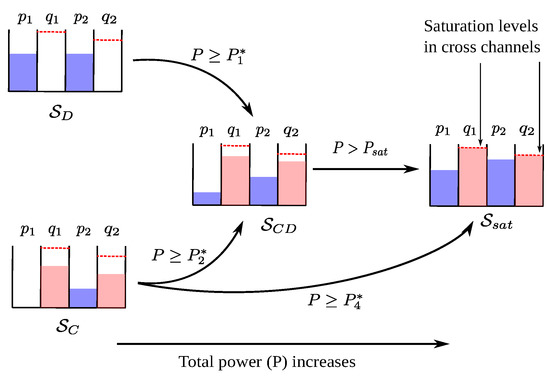
Figure 3. Due to its WF-like property, ${\mathbf{OA}}_{\mathbf{1}}$ follows one of the three sequences depending on $P_k^{*}$. The saturation levels in the cross channels are due to its max-min property.

• If $P_1^{*}>0$: ${\mathbf{OA}}_{\mathbf{1}}$ follows the sequence ${\mathcal{S}}_D\to {\mathcal{S}}_{CD}\to {\mathcal{S}}_{\mathsf{sat}}$ (denoted by [S1]). Since the direct channels are stronger, ${\mathbf{OA}}_{\mathbf{1}}$ allocates all of P to them as in ${\mathcal{S}}_D$ when P is sufficiently small (i.e., $P<P_1^{*}$). However, as P increases, the additional benefit from transmitting only in the direct channels decreases, and thus, when $P\ge P_1^{*}$, ${\mathbf{OA}}_{\mathbf{1}}$ begins transmitting in both cross and direct channels as in ${\mathcal{S}}_{CD}$. This allocation follows from its WF-like property, and remains optimal for all $P_1^{*}\le P\le P_3^{*}$. Finally, when $P>P_3^{*}$, the max-min property of ${\mathbf{OA}}_{\mathbf{1}}$ comes into effect, and thus the cross channels become saturated and ${\mathbf{OA}}_{\mathbf{1}}$ starts following the allocation in ${\mathcal{S}}_{\mathsf{sat}}$. Note that, in this case, the saturation threshold for P is $P_{\mathsf{sat}}=P_3^{*}$.
• If $P_2^{*}>0$ but $0<P_3^{*}<P_4^{*}<P_2^{*}$ is not satisfied: ${\mathbf{OA}}_{\mathbf{1}}$ follows the sequence ${\mathcal{S}}_C\to {\mathcal{S}}_{CD}\to {\mathcal{S}}_{\mathsf{sat}}$ ([S2]). This case is similar to [S1] above, except for the fact that now the cross channels are stronger. Hence, ${\mathbf{OA}}_{\mathbf{1}}$ transmits in the cross channels and the direct channel with gain $d_2^2$ as in ${\mathcal{S}}_C$ when P is sufficiently small (i.e., $P<min\{P_2^{*},P_4^{*}\}$). Next, following its WF-like property, ${\mathbf{OA}}_{\mathbf{1}}$ starts transmitting in all the direct and cross channels as in ${\mathcal{S}}_{CD}$ when $P\ge min\{P_2^{*},P_4^{*}\}$. Finally, when $P>max\{P_3^{*},P_4^{*}\},$ the cross channels become saturated, and ${\mathbf{OA}}_{\mathbf{1}}$ follows the allocation in ${\mathcal{S}}_{\mathsf{sat}}$ thereon. The saturation threshold for P in this case is $P_{\mathsf{sat}}=max\{P_3^{*},P_4^{*}\}$.
  Note that, whenever $P_2^{*}>0$, ${\mathbf{OA}}_{\mathbf{1}}$ follows [S2] irrespective of how $P_2^{*},P_3^{*}$, and $P_4^{*}$ compare, except in two cases: (a) $0<P_3^{*}<P_4^{*}<P_2^{*}$, where ${\mathbf{OA}}_{\mathbf{1}}$ follows [S3], described next, and (b) $0<P_4^{*}<P_3^{*}<P_2^{*}$, which is infeasible as they violate the mutual exclusiveness of ${\mathcal{S}}_C$ and ${\mathcal{S}}_{\mathsf{sat}}$.
• If $0<P_3^{*}<P_4^{*}<P_2^{*}$: ${\mathbf{OA}}_{\mathbf{1}}$ follows the sequence ${\mathcal{S}}_C\to {\mathcal{S}}_{\mathsf{sat}}$ ([S3]). In this case, the cross channels are much stronger than the direct channels. Hence, similar to [S2], ${\mathbf{OA}}_{\mathbf{1}}$ allocates power to both cross channels and a direct channel as in ${\mathcal{S}}_C$ when P is sufficiently small (i.e., $0\le P<P_4^{*}$). As P increases and $P\ge P_4^{*}$, the cross channels become saturated, and ${\mathbf{OA}}_{\mathbf{1}}$ begins assigning powers to all channels as in ${\mathcal{S}}_{\mathsf{sat}}$. Interestingly, in this case, ${\mathbf{OA}}_{\mathbf{1}}$ skips ${\mathcal{S}}_{CD}$. This shows that, since the cross channels are much stronger, it is optimal to allocate power as in ${\mathcal{S}}_C$ until they become saturated at $P_{\mathsf{sat}}=P_4^{*}$, beyond which the allocation in ${\mathcal{S}}_{\mathsf{sat}}$ becomes optimal.

We illustrate the characteristics of ${\mathbf{OA}}_{\mathbf{1}}$ with two numerical examples where we choose the following parameters, $a_{12}^2=a_{21}^2=1.5,Q_1=Q_2=5,\alpha =2,\beta =0.5$. First, we illustrate an example of [S1] by additionally choosing $d_1^2=2,d_2^2=3,c_{12}^2=1,c_{21}^2=1.5$, such that the direct channels are stronger than the cross channels in the sense that $P_1^{*}=0.619$ and $P_2^{*}=-0.75\notin {\mathbb{R}}_{+}$. In Figure 4a, we plot the optimal powers against the power budget P, and note the following: (i) when $0\le P<P_1^{*}=0.619$, ${\mathbf{OA}}_{\mathbf{1}}$ allocates P entirely to the direct channels as in ${\mathcal{S}}_D$, and thus $p_1$ and $p_2$ increase with P, and $q_1=q_2=0$; (ii) when $P_1^{*}\le P\le P_3^{*}=2.73$, ${\mathbf{OA}}_{\mathbf{1}}$ allocates power to all channels as in ${\mathcal{S}}_{CD}$, and thus $q_1$ and $q_2$ also increase with P; (iii) finally, when $P>P_3^{*}$, ${\mathbf{OA}}_{\mathbf{1}}$ follows ${\mathcal{S}}_{\mathsf{sat}}$ where the cross channels become saturated simultaneously, and all increments of P are added to $p_1$ and $p_2$.

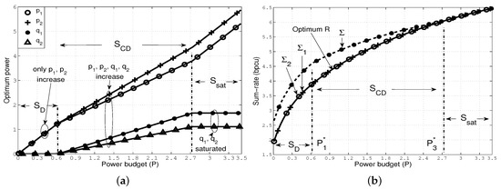
Figure 4. Optimal power allocation that follows the sequence [S1] ${\mathcal{S}}_D\to {\mathcal{S}}_{CD}\to {\mathcal{S}}_{\mathsf{sat}}.$ (a) optimal power allocation $(p_1,q_1,p_2,q_2)$; (b) the resulting sum-rate constraints.

We depict the resulting constraints ${\Sigma }_1,{\Sigma }_2$, and $\Sigma$ in Figure 4b. First, note that ${\mathbf{OA}}_{\mathbf{1}}$ preserves $R={\Sigma }_1={\Sigma }_2$ for all P. However, there exists a gap between ${\Sigma }_1={\Sigma }_2$ and $\Sigma$ in ${\mathcal{S}}_D$ and ${\mathcal{S}}_{CD}$. Specifically, in ${\mathcal{S}}_D$, the gap remains constant ($A-A_1$); in ${\mathcal{S}}_{CD},$ it reduces gradually as ${\mathbf{OA}}_{\mathbf{1}}$ transmits in the cross channels, and, in ${\mathcal{S}}_{\mathsf{sat}},$ it becomes zero as ${\mathbf{OA}}_{\mathbf{1}}$ achieves $R={\Sigma }_1={\Sigma }_2=\Sigma$, as expected.

Next, we illustrate an example of [S2] with the channel gains, $d_1^2=0.5,d_2^2=1,c_{12}^2=1.5,c_{21}^2=3,$ such that the cross channels are stronger than the direct channels in the sense that $P_2^{*}=0.22$ and $P_1^{*}=-0.21\notin {\mathbb{R}}_{+}$. In Figure 5a, we plot the optimal powers against P, and observe the following: (i) when $P<P_2^{*}=0.22$, ${\mathbf{OA}}_{\mathbf{1}}$ follows the allocation in ${\mathcal{S}}_C$, and thus $p_2$, $q_1$ and $q_2$ increase with P, whereas $p_1=0$; (ii) when $P_2^{*}\le P\le P_3^{*}=0.97$, ${\mathbf{OA}}_{\mathbf{1}}$ allocates power to all channels as in ${\mathcal{S}}_{CD}$, and thus $p_1$ now increases with P; (iii) finally, when $P>P_3^{*}$, ${\mathbf{OA}}_{\mathbf{1}}$ follows ${\mathcal{S}}_{\mathsf{sat}}$, and thus the cross channels become saturated simultaneously, as expected in [S2]. In Figure 5b, we plot the sum-rate constraints, and note that ${\mathbf{OA}}_{\mathbf{1}}$ achieves $R={\Sigma }_1={\Sigma }_2$ in all the sets. In addition, the gap between ${\Sigma }_1={\Sigma }_2$ and $\Sigma$ is gradually offset as ${\mathbf{OA}}_{\mathbf{1}}$ transmits in the cross channels in ${\mathcal{S}}_C$ and ${\mathcal{S}}_{CD}$, and it finally becomes zero in ${\mathcal{S}}_{\mathsf{sat}}$, as expected. We omit an example of [S3] (${\mathcal{S}}_C\to {\mathcal{S}}_{\mathsf{sat}}$), which is somewhat similar to [S2].

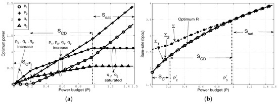
Figure 5. Optimal power allocation that follows the sequence [S2] ${\mathcal{S}}_C\to {\mathcal{S}}_{CD}\to {\mathcal{S}}_{\mathsf{sat}}.$ (a) optimal power allocation $(p_1,q_1,p_2,q_2)$; (b) the resulting sum-rate constraints.

Remark 1.

Recall that ${\mathbf{OA}}_{\mathbf{1}}$ presents the solution for $\left[\mathbf{P}\mathbf{1}\right]$ under $c_{12}^2<c_{21}^2$ and [A2] (implying $A_1=A_2$). If $c_{12}^2<c_{21}^2$ remains unchanged, and $\left[\mathbf{P}\mathbf{1}\right]$ is formulated under a more general assumption [A2G]; where $A_2<A_1$, then seven disjoint sets are needed to describe the optimal allocation (now denoted by ${\mathbf{OA}}_{\mathbf{G}}$). The conditions and power allocations of these sets are found by solving the corresponding KKT conditions in a similar way to that of $\left[\mathbf{P}\mathbf{1}\right]$ under [A2] in Appendix C. Hence, their explicit derivation is omitted for brevity. Of the seven sets, the first four sets, ${\widehat{\mathcal{S}}}_l$, $l\in \{D,C,CD,\mathsf{sat}\}$, are counterparts of the corresponding sets ${\mathcal{S}}_l$ in Table 1, in the sense that the power allocation in ${\widehat{\mathcal{S}}}_l$ is similar to that in ${\mathcal{S}}_l$ as discussed below. The remaining three sets ${\widehat{\mathcal{S}}}_k,k=1,2,3$ are “new” in the sense that the power allocation in these sets do not resemble that in any of the sets ${\mathcal{S}}_{(.)}$ in Table 1.

The power allocation in the first four sets ${\widehat{\mathcal{S}}}_l$ are similar to that of ${\mathcal{S}}_l,l\in \{D,C,CD,\mathsf{sat}\}$ in that (a) when the power budget (P) is sufficiently small, ${\mathbf{OA}}_{\mathbf{G}}$ allocates power to only both direct channels (in ${\widehat{\mathcal{S}}}_D$), or both cross channels and one direct channel (in ${\widehat{\mathcal{S}}}_C$) depending on whether the direct or the cross channels are “strong” as in ${\mathcal{S}}_D$ or ${\mathcal{S}}_C$ before; (b) as P is increased ${\mathbf{OA}}_{\mathbf{G}}$ allocates power to all channels (in ${\widehat{\mathcal{S}}}_{CD}$) as in ${\mathcal{S}}_{CD}$; and (c) when P is sufficiently large, both cross channels become saturated simultaneously, and ${\mathbf{OA}}_{\mathbf{G}}$ allocates all additional increments of P to only the direct channels (in ${\widehat{\mathcal{S}}}_{\mathsf{sat}}$) as in ${\mathcal{S}}_{\mathsf{sat}}$ before. Note that the optimal powers and the critical powers of ${\widehat{\mathcal{S}}}_{(.)}$ differ slightly from that of ${\mathcal{S}}_{(.)}$ due to the general assumption [A2G]. For conciseness, we omit the conditions, and present the optimal powers in Table 2.

Table 2. Optimal power allocation in the first four sets in ${\mathbf{OA}}_{\mathbf{G}}.$

Set		Optimal Powers
${\mathcal{S}}_D$	$p_1={\displaystyle \frac{P}{\beta }},$	$q_1=0,$	$p_2={\displaystyle \frac{P}{\beta }},$	$q_2=0,$
${\mathcal{S}}_C$	$p_1=0,$	$q_1={\displaystyle \frac{P}{\overline{\beta }}},$	$p_2={\displaystyle \frac{P{c}_{21}^2+\overline{\beta }-(P{c}_{12}^2+\overline{\beta })/\eta }{\beta c_{21}^2}},$	$q_2={\displaystyle \frac{P{c}_{12}^2/\overline{\beta }+1-\eta }{\eta c_{21}^2}},$
${\mathcal{S}}_{\mathsf{sat}}$	$p_1={\displaystyle \frac{P}{\beta }}-{\displaystyle \frac{\overline{\beta }(\gamma -1)}{\beta c_{12}^2}},$	$q_1={\displaystyle \frac{{\gamma }_1-1}{c_{12}^2}},$	$p_2={\displaystyle \frac{P}{\beta }}-{\displaystyle \frac{\overline{\beta }({\gamma }_2-1)}{\beta c_{21}^2}},$	$q_2={\displaystyle \frac{{\gamma }_2-1}{c_{21}^2}},$
${\mathcal{S}}_{CD}$	$p_1={\displaystyle \frac{P-\overline{\beta }{q}_1}{\beta }},$	$q_1={\displaystyle \frac{\widehat{F}(P)}{c_{12}^2}},$	$p_2={\displaystyle \frac{P-\overline{\beta }{q}_2}{\beta }},$	$q_2={\displaystyle \frac{1+c_{12}^2{q}_1}{\eta c_{21}^2}}-{\displaystyle \frac{1}{c_{21}^2}},$

Here ${\gamma }_k:={((1+Q_1)(1+Q_2)/(1+Q_l+a_{lk}^2{Q}_k))}^{1/\alpha \overline{\beta }},l\ne k\in \{1,2\}$, and $\widehat{F}(P)$ and η are defined in (39) and (40) below

$$\begin{array}{c}\widehat{F}(P):=\left(E_1+\eta E_2-\sqrt{{(E_1-\eta E_2)}^2+4{\beta }^2\eta E_1{E}_2}\right)/(2\overline{\beta }(1+\beta ))-1,\hfill \end{array}$$

(39)

$$\begin{array}{c}\eta :={\left(\frac{1+Q_1+a_{21}^2{Q}_2}{1+Q_2+a_{12}^2{Q}_1}\right)}^{1/\alpha \overline{\beta }}>1,\hfill \end{array}$$

(40)

with $E_1,E_2$, defined in (37). Note that, under [A2] ($\eta =1$), the powers in Table 2 simplifies to that in Table 1.

Next, we present the optimal powers and the critical powers of the three new sets in Table 3, where

$$\begin{array}{c}{P}_5^{*}:=\overline{\beta }\frac{(\eta -1)}{c_{12}^2},P_6^{*}:=\overline{\beta }\left(\frac{1}{d_1^2}-\frac{1}{c_{12}^2}\right),P_7^{*}:=\beta \left(\frac{1}{c_{12}^2}-\frac{1}{d_1^2}\right),P_8^{*}:=\frac{\eta -\overline{\beta }}{c_{12}^2}-\frac{\beta }{d_1^2},\hfill \\ f_3(P):=\frac{d_2^2}{c_{21}^2(1+d_2^{2}P/\beta )}+\frac{\beta \eta }{P{c}_{12}^2+\overline{\beta }+\beta c_{12}^2/d_1^2-\overline{\beta }\eta }.\hfill \end{array}$$

Table 3. Optimal power allocation and conditions of sets in ${\mathbf{OA}}_{\mathbf{S}}.$

Set	Optimal Powers				Condition
${\widehat{\mathcal{S}}}_1$	$p_1=0,$	$q_1={\displaystyle \frac{P}{\overline{\beta }}},$	$p_2={\displaystyle \frac{P}{\beta }},$	$q_2=0,$	$P\le P_5^{*},P<P_6^{*}$
${\widehat{\mathcal{S}}}_2$	$p_1=P+{\displaystyle \frac{\overline{\beta }}{c_{12}^2}}-{\displaystyle \frac{\overline{\beta }}{d_1^2}},$	$q_1=P+{\displaystyle \frac{\beta }{d_1^2}}-{\displaystyle \frac{\beta }{c_{12}^2}},$	$p_2={\displaystyle \frac{P}{\beta }},$	$q_2=0,$	$P>P_6^{*},P>P_7^{*},P<P_8^{*}$
${\widehat{\mathcal{S}}}_3$	$p_1={\displaystyle \frac{P}{\beta }}-{\displaystyle \frac{\overline{\beta }(\eta -1)}{\beta c_{12}^2}},$	$q_1={\displaystyle \frac{\eta -1}{c_{12}^2}},$	$p_2={\displaystyle \frac{P}{\beta }},$	$q_2=0,$	$P>P_5^{*},P\ge P_8^{*},f_3(P)>1$

The power allocation for the new sets can be understood by following the WF-like and max-min properties of ${\mathbf{OA}}_{\mathbf{G}}$. For illustration, we explain the allocations in ${\widehat{\mathcal{S}}}_1$ and ${\widehat{\mathcal{S}}}_2$. In ${\widehat{\mathcal{S}}}_1$, the cross channels are stronger than the direct channels. Thus, due to its WF-like property, ${\mathbf{OA}}_{\mathbf{G}}$ preferably allocates as much of P to the cross channels as possible. However, under [A2G] ($A_2<A_1$) and $c_{12}^2<c_{21}^2$, allocating power to both cross channels results in ${\Sigma }_2<{\Sigma }_1$, and does not increase $min\{{\Sigma }_2,{\Sigma }_1\}$ as much as possible. This results in a suboptimal sum-rate. Therefore, ${\mathbf{OA}}_{\mathbf{G}}$ allocates $p_1=0,q_1=P/\overline{\beta }$, which increases only ${\Sigma }_2$, and assigns $p_2=P/\beta ,q_2=0$, which represents the allocation in ${\widehat{\mathcal{S}}}_1$.

Furthermore, as P increases and $P>max\{P_6^{*},P_7^{*}\}$, additional benefits from transmitting only in the cross channel with gain $c_{12}^2$ reduces, and thus ${\mathbf{OA}}_{\mathbf{G}}$ starts allocating a fraction of P to the direct channel with gain $d_1^2$, due to its WF-like property. Thus, ${\mathbf{OA}}_{\mathbf{G}}$ follows the power allocation in ${\widehat{\mathcal{S}}}_2$, which remains optimal as long as $P<P_8^{*}$. The power allocation in ${\widehat{\mathcal{S}}}_3$ can be interpreted similarly.

The important insight is that ${\mathbf{OA}}_{\mathbf{G}}$ can be explained with the WF-like and max-min properties as in ${\mathbf{OA}}_{\mathbf{1}}$, and it does not reveal any new fundamental properties.

5.3. Optimum Power Allocation in the Symmetric DCLIC

We briefly discuss the optimum allocation for the symmetric DCLIC, where $a^2:=a_{12}^2=a_{21}^2$, $c^2:=c_{12}^2=c_{21}^2$, $d^2:=d_1^2=d_2^2$, and $Q_1=Q_2$. Due to symmetry, considering only symmetric power allocation of the form $(p,q,p,q)$ is sufficient, and does not cause loss of generality. Moreover, any feasible (symmetric) power allocation achieves ${\Sigma }_1={\Sigma }_2$, rendering the constraint $R\le {\Sigma }_2$ in (28) redundant. The sum-rate optimization problem in this case can be formulated and solved as in $\left[\mathbf{P}\mathbf{1}\right]$, and is omitted here for brevity. In addition, we denote the optimal power allocation for this case by ${\mathbf{OA}}_{\mathbf{S}}$.

In this case, ${\mathbf{OA}}_{\mathbf{S}}$ can be described by the power allocation in four disjoint sets, ${\overline{\mathcal{S}}}_l,l\in \{D,C,CD,\mathsf{sat}\}$, which are counterparts of the sets ${\mathcal{S}}_l$ in Table 1. The conditions and optimal powers in these sets are given in Table 4, and they can be derived following the same procedure as in Appendix C, and thus is omitted here.

Table 4. Optimal power allocation and conditions of sets in ${\mathbf{OA}}_{\mathbf{S}}.$

Set	Optimal Powers		Condition
${\overline{\mathcal{S}}}_D$	$p={\displaystyle \frac{P}{\beta }},$	$q=0,$	$P<{\overline{P}}_1^{*}$
${\overline{\mathcal{S}}}_C$	$p=0,$	$q={\displaystyle \frac{P}{\overline{\beta }}},$	$P<{\overline{P}}_2^{*},P<{\overline{P}}_4^{*}$
${\overline{\mathcal{S}}}_{CD}$	$p={\displaystyle \frac{2}{1+\beta }}\left(P+{\displaystyle \frac{\overline{\beta }}{c^2}}-{\displaystyle \frac{\overline{\beta }}{2d^2}}\right),$	$q={\displaystyle \frac{1}{1+\beta }}\left(P+{\displaystyle \frac{\beta }{d^2}}-{\displaystyle \frac{2\beta }{c^2}}\right),$	$P\ge {\overline{P}}_1^{*},P\ge {\overline{P}}_2^{*},P\le {\overline{P}}_3^{*}$
${\overline{\mathcal{S}}}_{\mathsf{sat}}$	$p={\displaystyle \frac{P}{\beta }}-{\displaystyle \frac{\overline{\beta }(\overline{\gamma }-1)}{\beta c^2}},$	$q={\displaystyle \frac{\overline{\gamma }-1}{c^2}}$,	$P\ge {\overline{P}}_4^{*},P>{\overline{P}}_3^{*}$

Moreover, the critical powers are now given by

$$\begin{array}{c}\hfill {\overline{P}}_1^{*}:=\beta \left(\frac{2}{c^2}-\frac{1}{d^2}\right),{\overline{P}}_2^{*}:=\frac{\overline{\beta }}{2}\left(\frac{1}{d^2}-\frac{2}{c^2}\right),{\overline{P}}_3^{*}:=\frac{(1+\beta )\overline{\gamma }}{c^2}-\frac{\beta }{d^2}-\frac{\overline{\beta }}{c^2},{\overline{P}}_4^{*}:=\frac{\overline{\beta }(\overline{\gamma }-1)}{c^2},\end{array}$$

where $\overline{\gamma }:={({(1+Q_1)}^2/(1+Q_1+a^2{Q}_1))}^{1/\alpha \overline{\beta }}>1$.

${\mathbf{OA}}_{\mathbf{S}}$ has the same WF-like and max-min properties as that of ${\mathbf{OA}}_{\mathbf{1}}$. In fact, a rudimentary inspection of the conditions reveals that ${\mathbf{OA}}_{\mathbf{S}}$ follows one of the three possible sequences of sets depending on the channel gains, as before:

• If $c^2\le 2d^2$ (direct channels are “stronger”): ${\mathbf{OA}}_{\mathbf{S}}$ follows the sequence ${\overline{\mathcal{S}}}_D\to {\overline{\mathcal{S}}}_{CD}\to {\overline{\mathcal{S}}}_{\mathsf{sat}}$. It transmits only in the direct channels as in ${\overline{\mathcal{S}}}_D$ when $P<{\overline{P}}_1^{*}$, then transmits in all channels as in ${\overline{\mathcal{S}}}_{CD}$ when ${\overline{P}}_1^{*}\le P\le P_3^{*}$, and finally starts following the allocation in ${\overline{\mathcal{S}}}_{\mathsf{sat}}$ when $P>{\overline{P}}_3^{*}$.
• If $2d^2<c^2<2d^2\overline{\gamma }$ (cross channels are “stronger”): ${\mathbf{OA}}_{\mathbf{S}}$ follows the sequence ${\overline{\mathcal{S}}}_C\to {\overline{\mathcal{S}}}_{CD}\to {\overline{\mathcal{S}}}_{\mathsf{sat}}$. It transmits only in the cross channels as in ${\overline{\mathcal{S}}}_C$ when $P<{\overline{P}}_2^{*}$, then transmits in all channels as in ${\overline{\mathcal{S}}}_{CD}$ when ${\overline{P}}_2^{*}\le P\le min\{P_3^{*},P_4^{*}\}$, and finally follows ${\overline{\mathcal{S}}}_{\mathsf{sat}}$ when $P>min\{P_3^{*},P_4^{*}\}$.
• If $c^2\ge 2d^2\overline{\gamma }$ (cross channels are much “stronger”): ${\mathbf{OA}}_{\mathbf{S}}$ follows the sequence ${\overline{\mathcal{S}}}_C\to {\overline{\mathcal{S}}}_{\mathsf{sat}}$. It follows ${\overline{\mathcal{S}}}_C$ when $P<{\overline{P}}_4^{*}$, and then follows ${\overline{\mathcal{S}}}_{\mathsf{sat}}$ when $P\ge P_4^{*}$, while skipping ${\overline{\mathcal{S}}}_{CD}$ altogether.

Thus, ${\mathbf{OA}}_{\mathbf{S}}$ allocates all of P to either both direct or both cross channels if P is small, and then shares P among all channels as P increases. In addition, when P is increased beyond the saturation threshold, the cross channels become saturated. Note that, due to symmetry, ${\mathbf{OA}}_{\mathbf{S}}$ needs to transmit in both cross channels only in ${\overline{\mathcal{S}}}_C$ to preserve ${\Sigma }_1={\Sigma }_2$, unlike in ${\mathcal{S}}_C$, where ${\mathbf{OA}}_{\mathbf{1}}$ additionally transmits in a direct channel.

We note the following, which are revealed due to symmetry. First, if $c^2<2d^2$, the direct channels are considered to be stronger than the cross channels. Similarly, if $c^2>2d^2$, the cross channels are considered to be stronger. Moreover, in the special case of $c^2=2d^2$, neither the direct nor the cross channels are stronger than the other, and thus allocating P entirely to only direct or cross channel would be suboptimal. Therefore, ${\mathbf{OA}}_{\mathbf{S}}$ transmits in all channels as in ${\mathcal{S}}_{CD}$ when $P\ge 0$. Finally, the condition $c^2\ge 2d^2\gamma$ implies that the cross channels are much stronger than the direct channels. Thus, it is optimal to transmit only in the cross channels as in ${\overline{\mathcal{S}}}_C$ until they become saturated, at which point the allocation in ${\overline{\mathcal{S}}}_{\mathsf{sat}}$ becomes optimal. Note that these conditions follow trivially from the corresponding conditions of [S1], [S2], and [S3] in Section 5.2 by applying symmetry.

Furthermore, due to symmetry, one can now directly observe that the conditions of the sets in Table 4 are mutually exclusive. For example, consider the conditions of ${\overline{\mathcal{S}}}_D$, $c^2<2d^2$ and $P<{\overline{P}}_1^{*}$, and note that they violate the second condition of ${\overline{\mathcal{S}}}_C$ (since ${\overline{P}}_2^{*}<0$), the first condition in ${\overline{\mathcal{S}}}_{CD}$ (since $P<{\overline{P}}_1^{*}$), and the second condition in ${\overline{\mathcal{S}}}_{\mathsf{sat}}$ (trivially follows from $\overline{\gamma }>1$).

In Figure 6, we depict the set of cross and direct channel gains ($c^2$ and $d^2$) of a symmetric DCLIC with parameters $a^2=1.5,Q_1=5,\alpha =2,\beta =0.5$, and partition it depending on whether the direct or the cross channels are stronger.

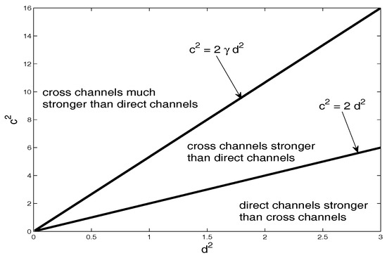
Figure 6. The set of all $c^2$ and $d^2$ is partitioned depending on whether the cross or the direct channels are “stronger”.

5.4. Discussion and Insights

Now, we discuss some insights obtained from the power allocation in ${\mathbf{OA}}_{\mathbf{1}}$ in Table 1.

First, if the underlying GIC in the first band has very strong interference, i.e., $a_{12}^2\ge 1+Q_1$ and $a_{21}^2\ge 1+Q_2$, ${\mathbf{OA}}_{\mathbf{1}}$ allocates the power budget (P) entirely to direct channels as in ${\mathcal{S}}_D$ for all values of P. Note that, under very strong interference, we have $\Sigma \le min\{{\Sigma }_1,{\Sigma }_2\}$ for any feasible power allocation. Therefore, the sum-rate is maximized by maximizing $\Sigma$, which is achieved by allocating all of P to the direct channels.

Second, if the transmit powers in the underlying GIC of the strong CLIC ($Q_1$ and $Q_2$) are small, i.e., $Q_1\approx 0,Q_2\approx 0$, then allocating P entirely to the direct channels as in ${\mathcal{S}}_D$, is approximately optimal for all values of P, in the sense that, the difference between the sum-rates achieved with the allocation in ${\mathcal{S}}_D$ and that in ${\mathbf{OA}}_{\mathbf{1}}$ is very small. Specifically, since $Q_1\approx 0,Q_2\approx 0$, the gap between $\Sigma$ and ${\Sigma }_1$ at $P=0$ is very small. As P is sufficiently increased, ${\mathbf{OA}}_{\mathbf{1}}$ starts transmitting in all channels as in ${\mathcal{S}}_{CD}$. However, since the gap is very small, only a small fraction of P needs to be allocated to the cross channels to offset the gap, and thus almost all of P is redirected to the direct channels. The resulting allocation closely resembles that in ${\mathcal{S}}_D$.

We can attribute this behavior of ${\mathbf{OA}}_{\mathbf{1}}$ to the fact that the GIC with strong interference ($a_{12}^2\ge 1,a_{21}^2\ge 1$) and small transmit powers ($Q_1\approx 0,Q_2\approx 0$) approaches the very strong interference regime ($a_{12}^2\ge 1+Q_1$, $a_{21}^2\ge 1+Q_2$), where allocating P entirely to the direct channels as in ${\mathcal{S}}_D$ is optimal for all P.

Third, if the transmit powers in the underlying GIC of the strong CLIC are large, i.e., $Q_1,Q_2\gg 1$, ${\mathbf{OA}}_{\mathbf{1}}$ allocates power in all channels as in ${\mathcal{S}}_{CD}$ for all but a relatively small range of P. Recall that even if ${\mathbf{OA}}_{\mathbf{1}}$ transmits in the direct or cross channels as in ${\mathcal{S}}_D$ or ${\mathcal{S}}_C$ for small P, eventually when $P\ge P_1^{*}$ or $P\ge P_2^{*}$, ${\mathbf{OA}}_{\mathbf{1}}$ allocates power in all channels as in ${\mathcal{S}}_{CD}$, where the gap between ${\Sigma }_1$ and $\Sigma$ starts to reduce. However, if $Q_1,Q_2\gg 1$, this gap is very large, and thus very large P is needed to offset the gap as in ${\mathcal{S}}_{\mathsf{sat}}$. Therefore, for all moderate P, ${\mathbf{OA}}_{\mathbf{1}}$ allocates power to all channels following ${\mathcal{S}}_{CD}$.

Fourth, if the cross channel gains in the second band are very large, allocating P entirely to the direct channels as in ${\mathcal{S}}_D$ is approximately optimal for all P, in the sense described in the second point above. This follows since with very large $c_{12}^2$ and $c_{21}^2$, ${\mathbf{OA}}_{\mathbf{1}}$ needs to allocate only a very small fraction of P to close the gap between ${\Sigma }_1$ and $\Sigma$, and thus redirects the remaining of P to the direct channels. The resulting allocation thus closely resembles that in ${\mathcal{S}}_D$.

Finally, when $\beta \approx 1$, the DCLIC can be approximated by the DLIC, and thus allocating P entirely to only the direct channels is approximately optimal. On the other hand, when $\beta \approx 0$, the DCLIC can be approximated by the CLIC where allocating P entirely to the cross channels is approximately optimal. However, since the cross channels do not increase $\Sigma$, the sum-rate becomes limited to $\Sigma$ when P is sufficiently large, and does not increase anymore.

6. Conclusions

Motivated by simultaneous transmission in the microwave and mm-wave bands, we considered a special class of dual band $2\times 2$ GIC. Due to their small wavelength and the use of highly directional antenna arrays, the mm-wave band can be used to form highly directional point-to-point links, allowing interference free reception at a designated receiver. For this model, we first showed that the capacity region of a DCLIC can be decomposed into the capacity of a CLIC complemented by direct channels. Moreover, we considered two specific classes of the CLIC with strong and weak underlying GIC, and obtained sufficient conditions on the channel gains under which the capacity region is characterized.

We characterized the power allocation over the mm-wave channels that maximizes the sum-rate of the DCLIC. Channel conditions have been characterized that determine how power is allocated to the channels depending on whether the direct or the cross channels are “strong”. In particular, the optimal allocation has a WF-like property due to which, when the power budget is small, it assigns the power budget entirely to either both direct channels, or both cross channels and at most one direct channel. As the power budget is increased, the optimal allocation eventually assigns power to all channels. It also has a max-min property, and, as a result, imposes a maximum limit on the cross-channel powers. This power allocation evaluates the impact of high bandwidth point-to-point mm-wave channels on the sum-rate performance, and thus can be useful in allocating resources in practice.

Potential future work includes analyzing other multi-user networks that operate with dual microwave and mm-wave bands.

References

- LTE-A 4G Solution, Stockholm, Sweden. Available online: https://www.ramonmillan.com/documentos/bibliografia/4GEricsson.pdf (accessed on 13 September 2017).
- Pi, Z.; Khan, F. An introduction to millimeter-wave mobile broadband systems. IEEE Commun. Mag. 2011, 49, 101–107. [Google Scholar] [CrossRef]
- Rappaport, T.S.; Sun, S.; Mayzus, R.; Zhao, H.; Azar, Y.; Wang, K.; Wong, G.N.; Schulz, J.K.; Samimi, M.; Gutierrez, F. Millimeter wave mobile communications for 5G cellular: It Will Work! IEEE Access 2013, 1, 335–349. [Google Scholar] [CrossRef]
- Akdeniz, M.R.; Liu, Y.; Samimi, M.K.; Sun, S.; Rangan, S.; Rappaport, T.S.; Erkip, E. Millimeter Wave Channel Modeling and Cellular Capacity Evaluation. IEEE J. Sel. Areas Commun. 2014, 32, 1164–1179. [Google Scholar] [CrossRef]
- Qingling, Z.; Li, J. Rain Attenuation in Millimeter Wave Ranges. In Proceedings of the IEEE 7th International Symposium on Antennas, Propagation and EM Theory, Guilin, China, 26–29 October 2006; pp. 1–4. [Google Scholar]
- Singh, S.; Mudumbai, R.; Madhow, U. Interference analysis for highly directional 60-GHz mesh networks: The case for rethinking medium access control. IEEE/ACM Trans. Netw. 2011, 19, 1513–1527. [Google Scholar] [CrossRef]
- Qiao, J.; Shen, X.S.; Mark, J.W.; Shen, Q.; He, Y.; Lei, L. Enabling device-to-device communications in millimeter-wave 5G cellular networks. IEEE Commun. Mag. 2015, 53, 209–215. [Google Scholar] [CrossRef]
- Collonge, S.; Zaharia, G.; Zein, G.E. Influence of the human activity on wide-band characteristics of the 60 GHz indoor radio channel. IEEE Trans. Wirel. Commun. 2004, 3, 2396–2406. [Google Scholar] [CrossRef]
- Zheng, K.; Zhao, L.; Mei, J.; Dohler, M.; Xiang, W.; Peng, Y. 10 Gb/s Hetsnets with Millimeter-wave communications: Access and networking - challenges and protocols. IEEE Commun. Mag. 2015, 53, 222–231. [Google Scholar] [CrossRef]
- G Radio Access: Requirements, Concept and Technologies. Available online: https://gsacom.com/paper/docomo-5g-radio-access-requirements-concept-and-technologies/ (accessed on 13 September 2017).
- Mehrpouyan, H.; Matthaiou, M.; Wang, R.; Karagiannidis, G.K.; Hua, Y. Hybrid millimeter-wave systems: A novel paradigm for hetnets. IEEE Commun. Mag. 2015, 53, 216–221. [Google Scholar] [CrossRef]
- Majhi, S.; Mitran, P. On the capacity of a class of dual-band interference channels. In Proceedings of the IEEE International Symposium on Information Theory, Barcelona, Spain, 10–15 July 2016; pp. 2759–2763. [Google Scholar]
- Feng, W.; Li, Y.; Jin, D.; Su, L.; Chen, S. Millimetre-wave backhaul for 5G networks: Challenges and solutions. Sensors 2016, 16, 892. [Google Scholar] [CrossRef] [PubMed]
- Morteza, H.; Koksal, C.E.; Shroff, N.B. Dual Sub-6 GHz—Millimeter Wave Beamforming and Communications to Achieve Low Latency and High Energy Efficiency in 5G Systems. Available online: https://arxiv.org/pdf/1701.06241.pdf (accessed on 13 September 2017).
- Niu, Y.; Li, Y.; Jin, D.; Su, L.; Vasilakos, A.V. A survey of millimeter wave communications (mmWave) for 5G: Opportunities and challenges. Wirel. Netw. 2015, 21, 2657–2676. [Google Scholar] [CrossRef]
- Intel Announces World’s First Global 5G Modem. Available online: https://newsroom.intel.com/newsroom/wp-content/uploads/sites/11/2017/01/5G-modem-fact-sheet.pdf (accessed on 13 September 2017).
- Ali, A.; González-Prelcic, N.; Heath, R.W. Estimating millimeter wave channels using out-of-band measurements. In Proceedings of the 2016 Information Theory and Applications Workshop, La Jolla, CA, USA, 31 January–5 February 2016; pp. 1–6. [Google Scholar]
- Ali, A.; Prelcic, N.; Robert, W.; Heath, J. Millimeter Wave Beam-Selection Using Out-of-Band Spatial Information. Available online: https://arxiv.org/pdf/1702.08574.pdf (accessed on 13 September 2017).
- Elshaer, H.; Kulkarni, M.N.; Boccardi, F.; Andrews, J.G.; Dohler, M. Downlink and uplink cell association with traditional macrocells and millimeter wave small cells. IEEE Trans. Wirel. Commun. 2016, 15, 6244–6258. [Google Scholar] [CrossRef]
- Semiari, O.; Saad, W.; Bennis, M. Joint millimeter wave and microwave resources allocation in cellular networks with dual-mode base stations. IEEE Trans. Wirel. Commun. 2017, 16, 4802–4816. [Google Scholar] [CrossRef]
- Rebato, M.; Boccardi, F.; Mezzavilla, M.; Rangan, S.; Zorzi, M. Hybrid spectrum sharing in mmwave cellular networks. IEEE Trans. Cogn. Commun. Netw. 2017, 3, 155–168. [Google Scholar] [CrossRef]
- Sato, H. The capacity of the Gaussian interference channel under strong interference. IEEE Trans. Inf. Theory 1981, 27, 786–788. [Google Scholar] [CrossRef]
- Carleial, A. A case where interference does not reduce capacity. IEEE Trans. Inf. Theory 1975, 21, 569–570. [Google Scholar] [CrossRef]
- Kramer, G. Outer bounds on the capacity of Gaussian interference channels. IEEE Trans. Inf. Theory 2004, 50, 581–586. [Google Scholar] [CrossRef]
- Chung, S.T.; Cioffi, J. The capacity region of frequency-selective Gaussian interference channels under strong interference. IEEE Trans. Commun. 2007, 55, 1812–1821. [Google Scholar] [CrossRef]
- Choi, S.W.; Chung, S.Y. On the separability of parallel Gaussian interference channels. In Proceedings of the IEEE International Symposium on Information Theory, Seoul, South Korea, 28 June–3 July 2009; pp. 2592–2596. [Google Scholar]
- Sankar, L.; Shang, X.; Erkip, E.; Poor, H.V. Ergodic fading interference channels: Sum-capacity and separability. IEEE Trans. Inf. Theory 2011, 57, 2605–2626. [Google Scholar] [CrossRef]
- Cadambe, V.; Jafar, S. Parallel Gaussian interference channels are not always separable. IEEE Trans. Inf. Theory 2009, 55, 3983–3990. [Google Scholar] [CrossRef]
- Shang, X.; Chen, B.; Kramer, G.; Poor, H. Noisy-interference sum-rate capacity of parallel Gaussian interference channels. IEEE Trans. Inf. Theory 2011, 57, 210–226. [Google Scholar] [CrossRef]
- Yu, W.; Ginis, G.; Cioffi, J.M. Distributed multiuser power control for digital subscriber lines. IEEE J. Sel. Areas Commun. 2002, 20, 1105–1115. [Google Scholar] [CrossRef]
- Chen, H.; Ma, Y.; Lin, Z.; Li, Y.; Vucetic, B. Distributed power control in interference channels with QoS constraints and RF energy harvesting: A game-theoretic approach. IEEE Trans. Veh. Technol. 2016, 65, 10063–10069. [Google Scholar] [CrossRef]
- Gamal, A.E.; Kim, Y.H. Network Information Theory; Cambridge University Press: Cambridge, UK, 2012. [Google Scholar]
- Diggavi, S.N.; Cover, T.M. The worst additive noise under a covariance constraint. IEEE Trans. Inf. Theory 2006, 47, 3072–3081. [Google Scholar] [CrossRef]
- Sankar, L.; Liang, Y.; Mandayam, N.B.; Poor, H.V. Fading multiple access relay channels: Achievable rates and opportunistic scheduling. IEEE Trans. Inf. Theory 2011, 57, 1911–1931. [Google Scholar] [CrossRef]
- Boyd, S.; Vandenberghe, L. Convex Optimization; Cambridge University Press: Cambridge, UK, 2004. [Google Scholar]
© 2017 by the authors. Licensee MDPI, Basel, Switzerland. This article is an open access article distributed under the terms and conditions of the Creative Commons Attribution (CC BY) license (http://creativecommons.org/licenses/by/4.0/).