Rolling Bearing Diagnosis Based on Composite Multiscale Weighted Permutation Entropy


Abstract
:1. Introduction
2. MPE, MWPE, CMWPE
2.1. MPE
2.1.1. PE
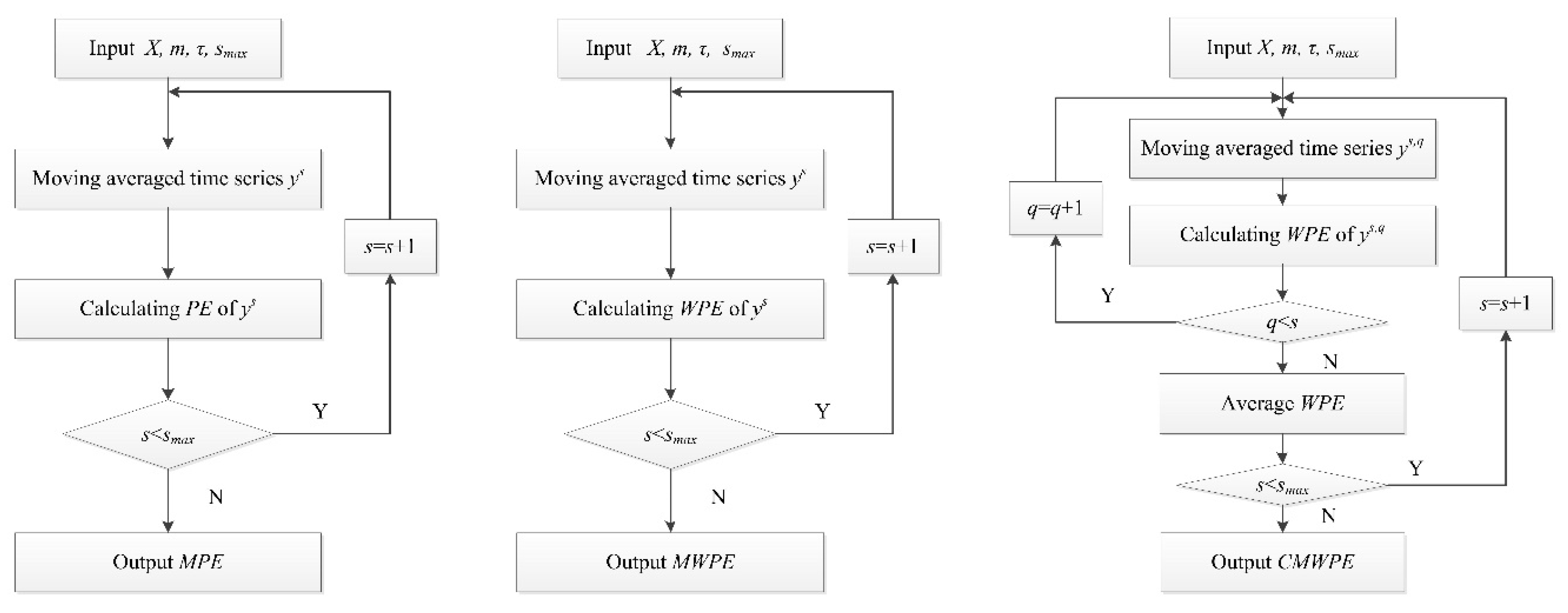
2.1.2. MPE
2.2. MWPE
2.2.1. WPE
2.2.2. MWPE
2.3. CMWPE
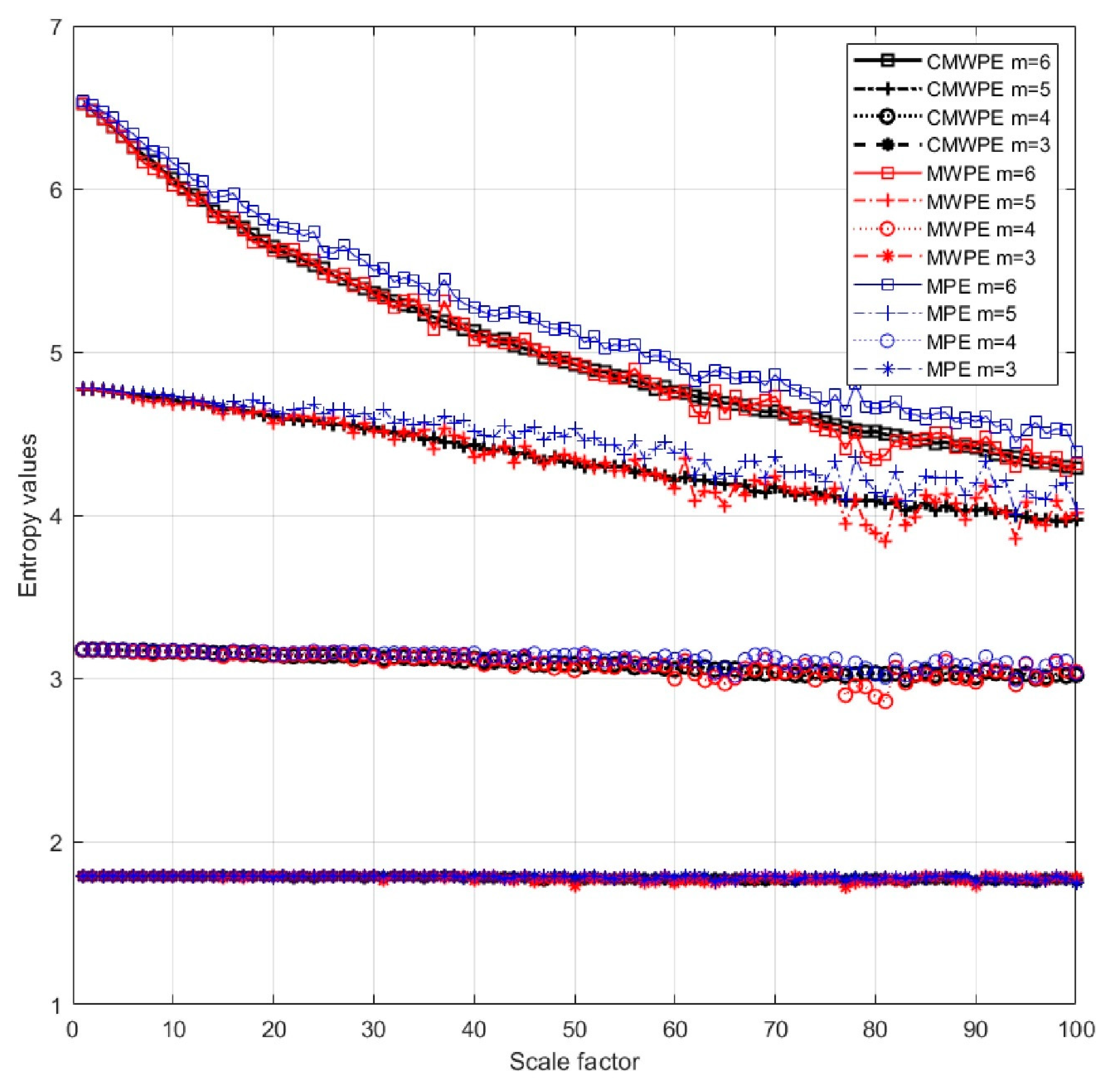
2.4. Comparisons between MPE, MWPE, CMWPE
3. Fault Diagnosis Approach Based on CMWPE, JMI, and KNN
3.1. JMI Feature Selection
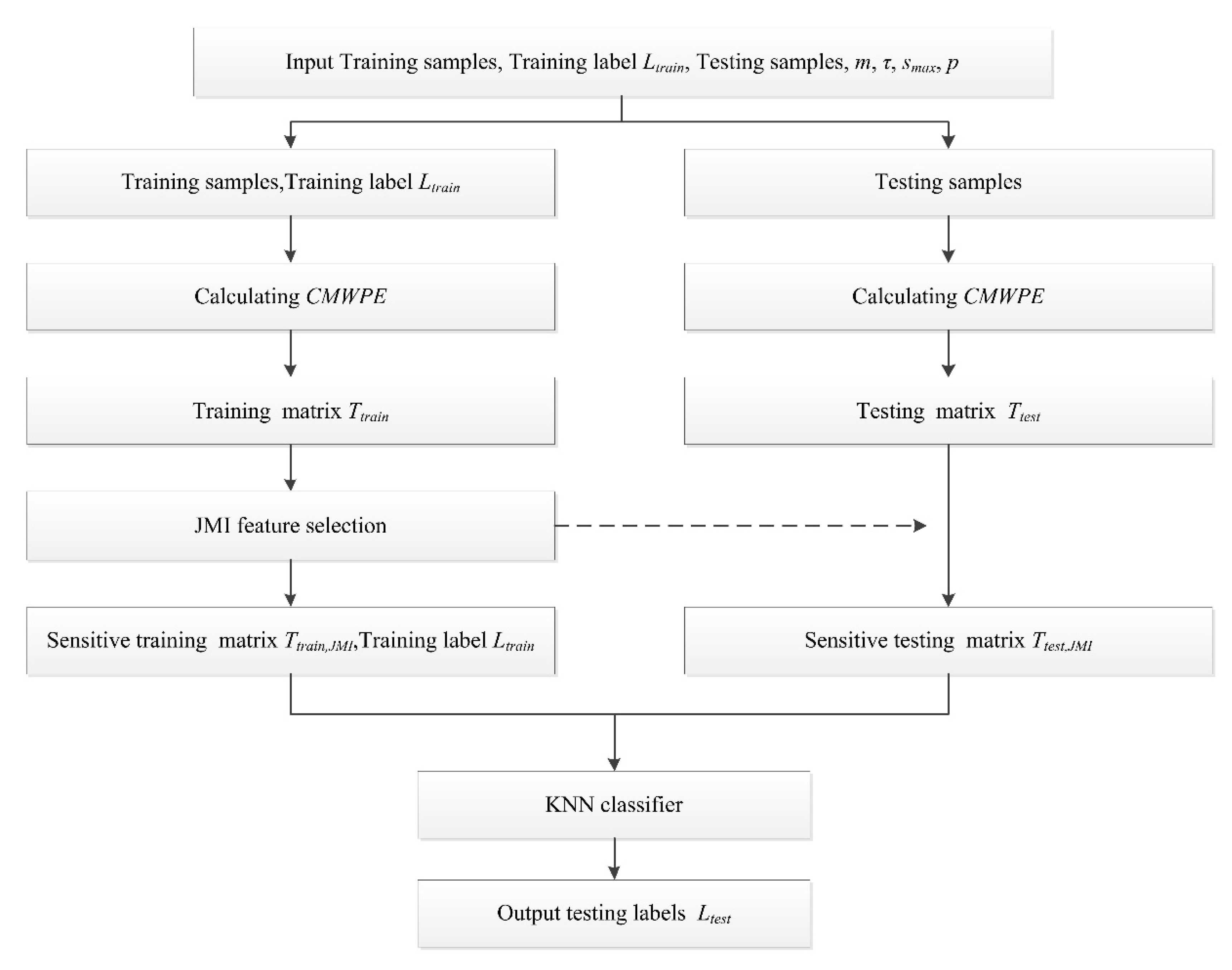
3.2. CMWPE-JMI-KNN
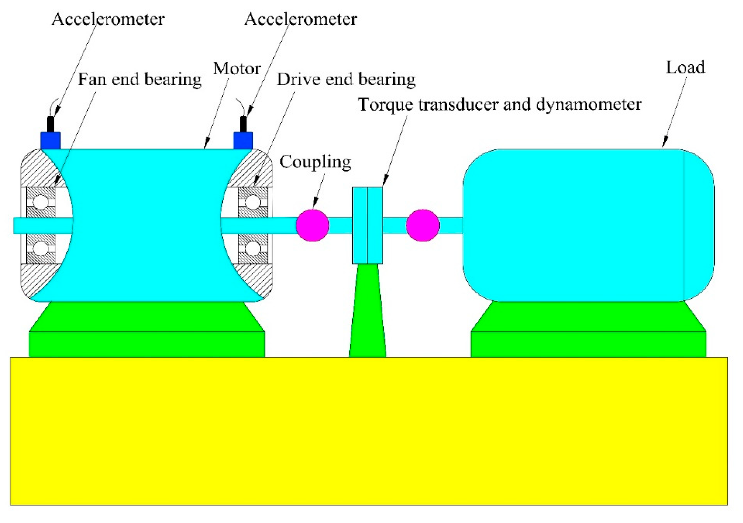
4. Experimental Validation
5. Conclusions
- Combining entropy theories and advanced signal processing techniques to further improve the recognition accuracy and anti-noise ability.
- Applying the proposed diagnosis method to more types of mechanical fault diagnosis in real world industrial applications.
Author Contributions
Funding
Conflicts of Interest
References
- Zheng, J.; Cheng, J.; Yang, Y. A rolling bearing fault diagnosis approach based on LCD and fuzzy entropy. Mech. Mach. Theory 2013, 70, 441–453. [Google Scholar] [CrossRef]
- Gong, H.; Huang, W.; Zhao, K.; Li, S.; Zhu, Z. Time-frequency feature extraction based on fusion of Wigner-Ville distribution and wavelet scalogram. J. Vib. Eng. 2011, 30, 35–38. [Google Scholar]
- Gao, H.; Liang, L.; Chen, X.; Xu, G. Feature extraction and recognition for rolling element bearing fault utilizing short-time Fourier transform and non-negative matrix factorization. Chin. J. Mech. Eng. 2015, 28, 96–105. [Google Scholar] [CrossRef]
- Rodriguez, N.; Cabrera, G.; Lagos, C.; Cabrera, E. Stationary Wavelet Singular Entropy and Kernel Extreme Learning for Bearing Multi-Fault Diagnosis. Entropy 2017, 19, 541. [Google Scholar] [CrossRef]
- Lei, Y.; Lin, J.; He, Z.; Zuo, M.J. A review on empirical mode decomposition in fault diagnosis of rotating machinery. Mech. Syst. Signal Process. 2013, 35, 108–126. [Google Scholar] [CrossRef]
- Li, Y.; Xu, M.; Wei, Y.; Huang, W. An improvement EMD method based on the optimized rational Hermite interpolation approach and its application to gear fault diagnosis. Measurement 2015, 63, 330–345. [Google Scholar] [CrossRef]
- Zhang, Y.; Qin, Y.; Xing, Z.; Jia, L.; Cheng, X. Roller bearing safety region estimation and state identification based on LMD–PCA–LSSVM. Measurement 2013, 46, 1315–1324. [Google Scholar] [CrossRef]
- Liu, H.; Han, M. A fault diagnosis method based on local mean decomposition and multi-scale entropy for roller bearings. Mech. Mach. Theory 2014, 75, 67–78. [Google Scholar] [CrossRef]
- Zhang, L.; Li, P.; Li, M.; Zhang, S.; Zhang, Z. Fault diagnosis of rolling bearing based on ITD fuzzy entropy and GG clustering. Chin. J. Sci. Instrum. 2014, 35, 2624–2632. [Google Scholar]
- Yang, Y.; Pan, H.; Ma, L.; Cheng, J. A roller bearing fault diagnosis method based on the improved ITD and RRVPMCD. Measurement 2014, 55, 255–264. [Google Scholar] [CrossRef]
- Lu, C.; Wang, Y.; Ragulskis, M.; Cheng, Y. Fault Diagnosis for Rotating Machinery: A Method based on Image Processing. PLoS ONE 2016, 11, e0164111. [Google Scholar] [CrossRef] [PubMed]
- Zhao, L.Y.; Wang, L.; Yan, R.Q. Rolling Bearing Fault Diagnosis Based on Wavelet Packet Decomposition and Multi-Scale Permutation Entropy. Entropy 2015, 17, 6447–6461. [Google Scholar] [CrossRef] [Green Version]
- He, W.; Zi, Y.; Chen, B.; Wu, F.; He, Z. Automatic fault feature extraction of mechanical anomaly on induction motor bearing using ensemble super-wavelet transform. Mech. Syst. Signal Process. 2015, 54–55, 457–480. [Google Scholar] [CrossRef]
- Pincus, S. Approximate entropy (ApEn) as a complexity measure. Chaos 1995, 5, 110–117. [Google Scholar] [CrossRef] [PubMed]
- Li, Q.; Wang, T.Y.; Xu, Y.G.; He, H.L.; Zhang, Y. Fault diagnosis of rolling bearings based on chaos and two-dimensional approximate Entropy. J. Vib. Eng. 2007, 20, 268–273. [Google Scholar]
- Richman, J.S.; Moorman, J.R. Physiological time-series analysis using approximate entropy and sample entropy. Am. J. Physiol.-Heart C 2000, 278, H2039–H2049. [Google Scholar] [CrossRef] [PubMed]
- Zhao, Z.H.; Yang, S.P. Sample entropy-based roller bearing fault diagnosis method. J. Vib. Shock 2012, 31, 136–154. [Google Scholar]
- Costa, M.; Goldberger, A.L.; Peng, C.K. Multiscale Entropy Analysis of Complex Physiologic Time Series. Phys. Rev. Lett. 2007, 89, 705–708. [Google Scholar] [CrossRef] [PubMed]
- Jinde, Z.; Junsheng, C.; Yang, Y. A rolling bearing fault diagnosis approach based on multiscale entropy. J. Hum. Univ. 2012, 39, 38–41. [Google Scholar]
- Bandt, C.; Pompe, B. Permutation Entropy: A Natural Complexity Measure for Time Series. Phys. Rev. Lett. 2002, 88, 174102. [Google Scholar] [CrossRef] [PubMed]
- Rao, G.Q.; Feng, F.Z.; Si, A.W.; Xie, J.L. Method for optimal determination of parameters in permutation entropy algorithm. J. Vib. Shock 2014, 33, 188–193. [Google Scholar]
- Duan, L.; Xiaoli, L.; Zhenhu, L.; Logan, J.V.; Jamie, W.S. Multiscale permutation entropy analysis of EEG recordings during sevoflurane anesthesia. J. Neural Eng. 2010, 7, 046010. [Google Scholar] [CrossRef]
- Li, Y.; Xu, M.; Wei, Y.; Huang, W. A new rolling bearing fault diagnosis method based on multiscale permutation entropy and improved support vector machine based binary tree. Measurement 2016, 77, 80–94. [Google Scholar] [CrossRef]
- Fadlallah, B.; Chen, B.; Keil, A.; Príncipe, J. Weighted-permutation entropy: A complexity measure for time series incorporating amplitude information. Phys. Rev. E 2013, 87, 022911. [Google Scholar] [CrossRef] [PubMed]
- Yin, Y.; Shang, P. Weighted multiscale permutation entropy of financial time series. Nonlinear Dyn. 2014, 78, 2921–2939. [Google Scholar] [CrossRef]
- Wu, S.D.; Wu, C.W.; Lin, S.G.; Wang, C.C.; Lee, K.Y. Time Series Analysis Using Composite Multiscale Entropy. Entropy 2013, 15, 1069–1084. [Google Scholar] [CrossRef] [Green Version]
- Zheng, J.; Pan, H.; Cheng, J. Rolling bearing fault detection and diagnosis based on composite multiscale fuzzy entropy and ensemble support vector machines. Mech. Syst. Signal Process. 2017, 85, 746–759. [Google Scholar] [CrossRef]
- Yin, Y.; Shang, P. Multivariate weighted multiscale permutation entropy for complex time series. Nonlinear Dyn. 2017, 88, 1707–1722. [Google Scholar] [CrossRef]
- Yang, H.; Moody, J. Data Visualization and Feature Selection: New Algorithms for Nongaussian Data. Adv. Neural Inf. Process. Syst. 2000, 2, 687–693. [Google Scholar]
- Sheng, S.; Yang, H.; Wang, Y.; Pan, Y.; Tang, J. Joint mutual information feature selection for underwater acoustic targets. J. Northwest. Polytech. Univ. 2015, 33, 639–643. [Google Scholar]
- Bearing Data Center, Case Western Reserve University. Available online: http://csegroups.case.edu/bearingdatacenter/pages/download-data-file (accessed on 23 October 2018).


| Bearing Condition | Fault Diameter (mm) | Motor Load (HP) | Motor Speed (rpm) | Label | Number of Training Samples | Number of Testing Samples |
|---|---|---|---|---|---|---|
| Normal | 0 | 0 | 1772 | 1 | 22 | 88 |
| IRF1 | 0.1778 | 0 | 1772 | 2 | 22 | 88 |
| BF1 | 0.1778 | 0 | 1772 | 3 | 22 | 88 |
| ORF1 | 0.1778 | 0 | 1772 | 4 | 22 | 88 |
| IRF2 | 0.3556 | 0 | 1772 | 5 | 22 | 88 |
| BF2 | 0.3556 | 0 | 1772 | 6 | 22 | 88 |
| ORF2 | 0.3556 | 0 | 1772 | 7 | 22 | 88 |
| IRF3 | 0.5334 | 0 | 1772 | 8 | 22 | 88 |
| BF3 | 0.5334 | 0 | 1772 | 9 | 22 | 88 |
| ORF3 | 0.5334 | 0 | 1772 | 10 | 22 | 88 |
| Experiments | CMWPE-JMI-KNN | MWPE-JMI-KNN | MPE-JMI-KNN | ||||||
|---|---|---|---|---|---|---|---|---|---|
| Accuracy (%) | Accuracy (%) | Accuracy (%) | |||||||
| Max | Min | Mean | Max | Min | Mean | Max | Min | Mean | |
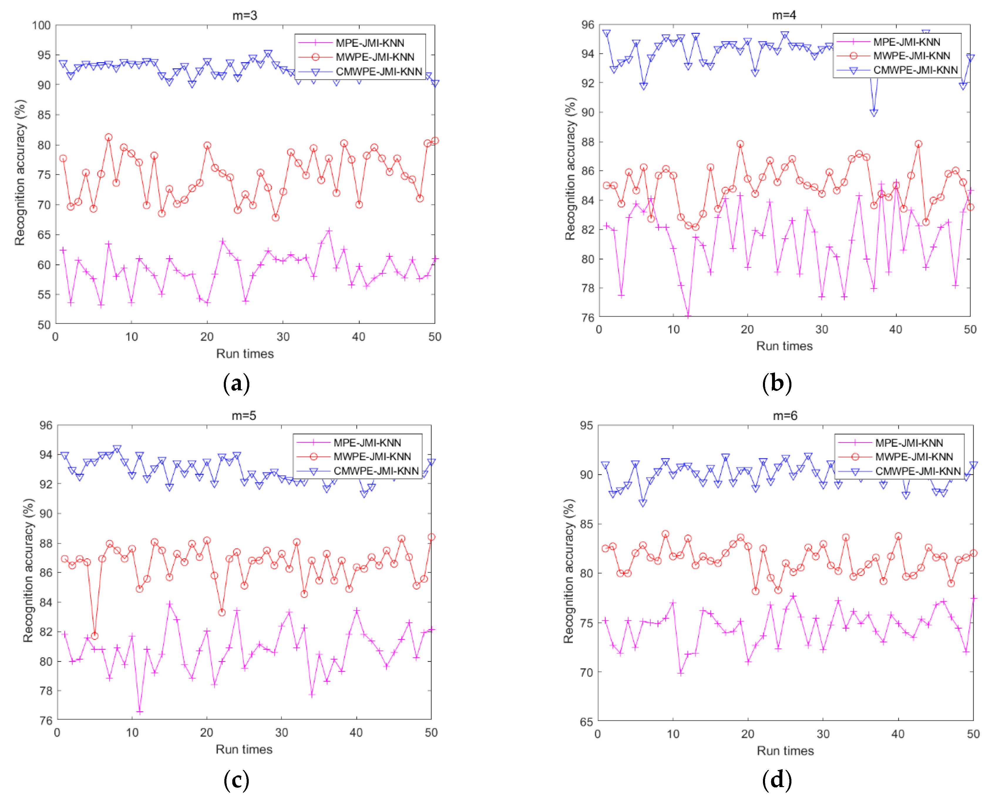
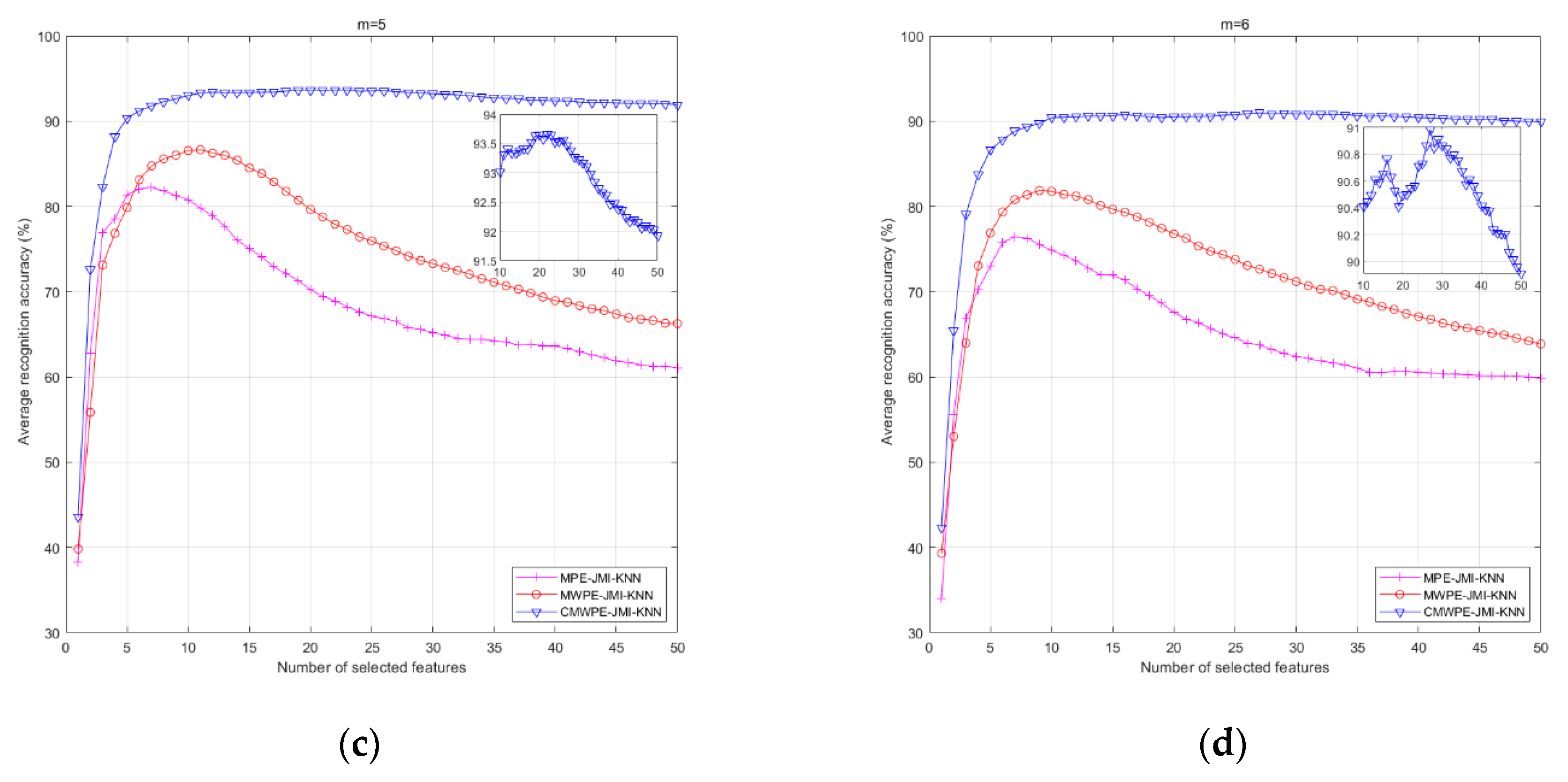
| m = 3 | 95.34 | 90.22 | 92.70 | 81.25 | 67.84 | 74.79 | 65.68 | 53.18 | 59.13 |
| m = 4 | 95.45 | 90.00 | 94.11 | 87.84 | 82.15 | 85.00 | 85.22 | 76.13 | 81.35 |
| m = 5 | 94.43 | 91.36 | 93.01 | 88.40 | 81.70 | 86.56 | 83.86 | 76.59 | 80.79 |
| m = 6 | 93.06 | 87.15 | 90.17 | 83.97 | 78.18 | 81.38 | 77.72 | 69.88 | 74.55 |
| Experiments | CMWPE-RANDOM-KNN | MWPE-RANDOM-KNN | MPE-RANDOM-KNN | ||||||
|---|---|---|---|---|---|---|---|---|---|
| Accuracy (%) | Accuracy (%) | Accuracy (%) | |||||||
| Max | Min | Mean | Max | Min | Mean | Max | Min | Mean | |
| m = 3 | 87.95 | 40.68 | 67.10 | 44.43 | 14.31 | 25.88 | 38.97 | 10.45 | 19.74 |
| m = 4 | 89.43 | 54.20 | 72.18 | 49.43 | 13.40 | 27.48 | 48.63 | 8.63 | 22.02 |
| m = 5 | 86.47 | 46.70 | 69.56 | 52.72 | 13.75 | 29.57 | 56.93 | 10.00 | 23.91 |
| m = 6 | 84.09 | 48.18 | 65.48 | 53.86 | 16.36 | 31.15 | 52.15 | 11.81 | 24.94 |
© 2018 by the authors. Licensee MDPI, Basel, Switzerland. This article is an open access article distributed under the terms and conditions of the Creative Commons Attribution (CC BY) license (http://creativecommons.org/licenses/by/4.0/).
Share and Cite
Gan, X.; Lu, H.; Yang, G.; Liu, J. Rolling Bearing Diagnosis Based on Composite Multiscale Weighted Permutation Entropy. Entropy 2018, 20, 821. https://doi.org/10.3390/e20110821
Gan X, Lu H, Yang G, Liu J. Rolling Bearing Diagnosis Based on Composite Multiscale Weighted Permutation Entropy. Entropy. 2018; 20(11):821. https://doi.org/10.3390/e20110821
Chicago/Turabian StyleGan, Xiong, Hong Lu, Guangyou Yang, and Jing Liu. 2018. "Rolling Bearing Diagnosis Based on Composite Multiscale Weighted Permutation Entropy" Entropy 20, no. 11: 821. https://doi.org/10.3390/e20110821