1. Introduction
The brain receives various information from the external world. Integrating this information is an essential property for cognition and consciousness [
1]. In fact, phenomenologically, our consciousness is unified. For example, when we see an object, we cannot experience only its shape independently of its color. Conversely, we cannot experience only the left half of the visual field independently of the right half. Integrated Information Theory (IIT) of consciousness considers that the unification of consciousness should be realized by the ability of the brain to integrate information [
2,
3,
4]. That is, the brain has internal mechanisms to integrate information about the shape and color of an object or information of the right and left visual field, and therefore our visual experiences are unified. IIT proposes to quantify the degree of information integration by an information theoretic measure “integrated information” and hypothesizes that integrated information is related to the level of consciousness. Although the hypothesis is indirectly supported by experiments which showed the breakdown of effective connectivity in the brain during loss of consciousness [
5,
6], only a few studies have directly quantified integrated information in real neural data [
7,
8,
9,
10] because of the computational difficulties described below.
Conceptually, integrated information quantifies the degree of interaction between parts or equivalently, the amount of information loss caused by splitting a system into parts [
11,
12]. IIT proposes that integrated information should be quantified between the least interdependent parts so that it quantifies information integration in a system as a whole. For example, if a system consists of two independent subsystems, the two subsystems are the least interdependent parts. In this case, integrated information is 0, because there is no information loss when the system is partitioned into the two independent subsystems. Such a critical partition of the system is called the Minimum Information Partition (MIP), where information is minimally lost, or equivalently where integrated information is minimized. In general, searching for the MIP requires an exponentially large amount of computational time because the number of partitions exponentially grows with the arithmetic growth of system size
N. This computational difficulty hinders the application of IIT to experimental data, despite its potential importance in consciousness research and even in broader fields of neuroscience.
In the present study, we exploit a mathematical concept called submodularity to resolve the combinatorial explosion of finding the MIP. Submodularity is an important concept in set functions which is analogous to convexity in continuous functions. It is known that an exponentially large computational cost for minimizing an objective function is reduced to the polynomial order if the objective function satisfies submodularity. Previously, Hidaka and Oizumi showed that the computational cost for finding the MIP is reduced to
[
13] by utilizing Queyranne’s submodular optimization algorithm [
14]. They used mutual information as a measure of integrated information that satisfies submodularity. The measure of integrated information used in the first version of IIT (IIT 1.0) [
2] is based on mutual information. Thus, if we consider mutual information as a practical approximation of the measure of integrated information in IIT 1.0, Queyranne’s algorithm can be utilized for finding the MIP. However, the practical measures of integrated information in the later versions of IIT [
12,
15,
16,
17] are not submodular.
In this paper, we aim to extend the applicability of submodular optimization to non-submodular measures of integrated information. We specifically consider the three measures of integrated information: mutual information
[
2], stochastic interaction
[
15,
18,
19], and geometric integrated information
[
12]. Mutual information is strictly submodular but the others are not. Oizumi et al. previously showed a close relationship among these three measures [
12,
20]. From this relationship, we speculate that Queyranne’s algorithm might work well for the non-submodular measures. Here, we empirically explore to what extent Queyranne’s algorithm can be applied to the two non-submodular measures of integrated information by evaluating the accuracy of the algorithm in simulated data and real neural data. We find that Queyranne’s algorithm identifies the MIP in a nearly perfect manner even for the non-submodular measures. Our results show that Queyranne’s algorithm can be utilized even for non-submodular measures of integrated information and makes it possible to practically compute integrated information across the MIP in real neural data, such as multi-unit recordings used in Electroencephalography (EEG) and Electrocorticography (ECoG), which typically consist of around 100 channels. Although the MIP was originally proposed in IIT for understanding consciousness, it can be utilized to analyze any system irrespective of consciousness such as biological networks, multi-agent systems, and oscillator networks. Therefore, our work would be beneficial not only for consciousness studies but also to other research fields involving complex networks of random variables.
This paper is organized as follows. We first explain that the three measures of integrated information,
,
, and
, are closely related from a unified theoretical framework [
12,
20] and there is an order relation among the three measures:
. Next, we compare the partition found by Queyranne’s algorithm with the MIP found by exhaustive search in randomly generated small networks (
). We also evaluate the performance of Queyranne’s algorithm in larger networks (
and 50 for
and
, respectively). Since the exhaustive search is intractable, we compare Queyranne’s algorithm with a different optimization algorithm called the replica exchange Markov Chain Monte Carlo (REMCMC) method [
21,
22,
23,
24]. Finally, we evaluate the performance of Queyranne’s algorithm in ECoG data recorded in monkeys and investigate the applicability of the algorithm in real neural data.
2. Measures of Integrated Information
Let us consider a stochastic dynamical system consisting of
N elements. We represent the past and present states of the system as
and
, respectively. In the case of a neural system, the variable
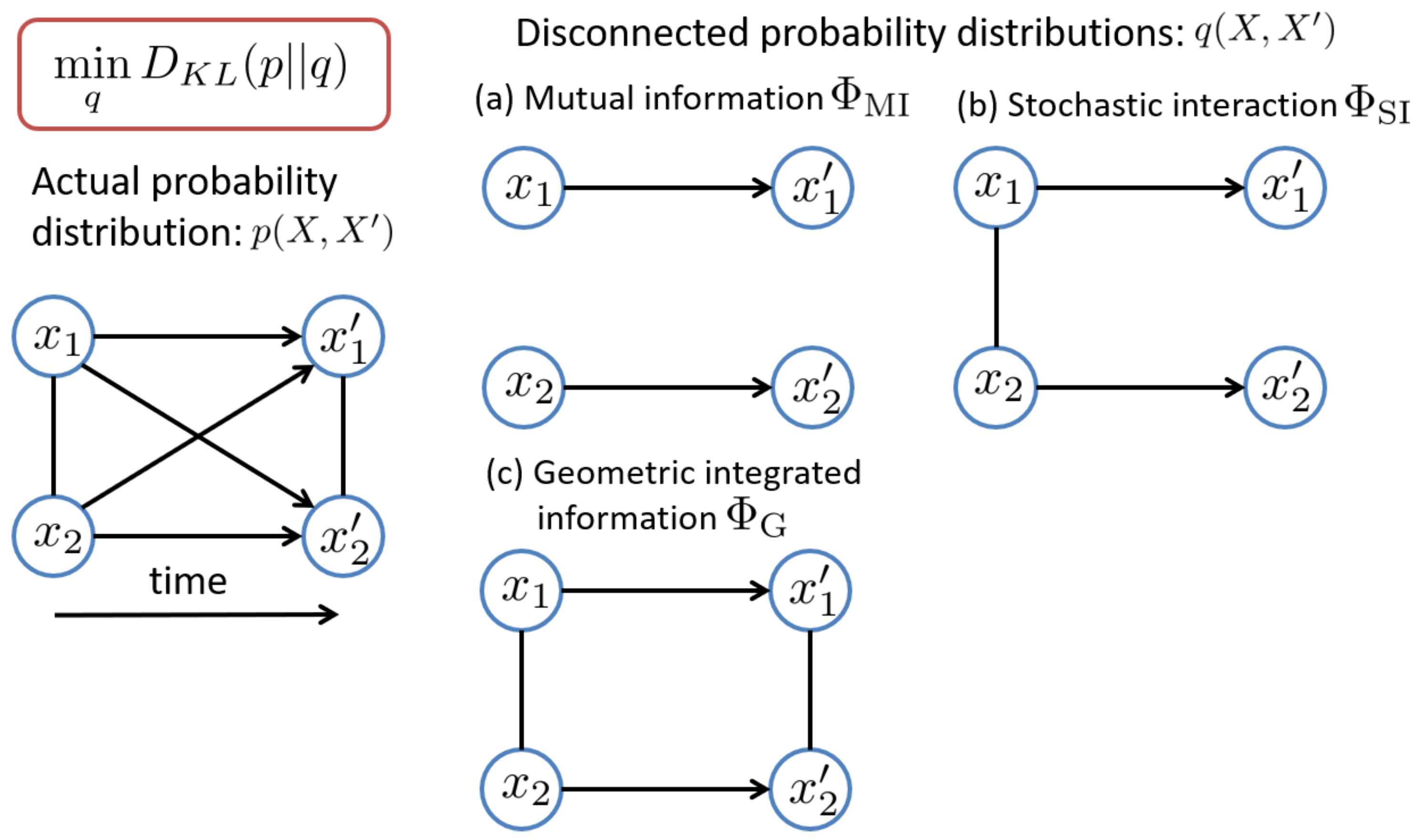
X can be signals of multi-unit recordings, EEG, ECoG, functional magnetic resonance imaging (fMRI), etc. Conceptually, integrated information is designed to quantify the degree of spatio-temporal interactions between subsystems. The previously proposed measures of integrated information are generally expressed as the Kullback–Leibler divergence between the actual probability distribution
and a “disconnected” probability distribution
where interactions between subsystems are removed [
12].
The Kullback–Leibler divergence measures the difference between the probability distributions, and can be interpreted as the information loss when
is used to approximate
[
25]. Thus, integrated information is interpreted as information loss caused by removing interactions. In Equation (
2), the minimum over
q should be taken to find the best approximation of
p, while satisfying the constraint that the interactions between subsystems are removed [
12].
There are many ways of removing interactions between units, which lead to different disconnected probability distributions
q, and also different measures of integrated information (
Figure 1). The arrows indicate influences across different time points and the lines without arrowheads indicate influences between elements at the same time. Below, we will show that three different measures of integrated information are derived from different probability distributions
q.
2.1. Multi (Mutual) Information
First, consider the following partitioned probability distribution
q,
where the whole system is partitioned into
K subsystems and the past and present states of the
i-th subsystem are denoted by
and
, respectively, i.e.,
and
. Each subsystem consists of one or multiple elements. The distribution
is the marginalized distribution
where
and
are the complement of
and
, that is,
and
, respectively. In this model, all of the interactions between the subsystems are removed, i.e., the subsystems are totally independent (
Figure 1a). In this case, the corresponding measure of integrated information is given by
where
represents the joint entropy. This measure is called total correlation [
26] or multi information [
27]. As a special case when the number of subsystems is two, this measure is simply equivalent to the mutual information between the two subsystems,
The measure of integrated information used in the first version of IIT is based on mutual information but is not identical to mutual information in Equation (
6). The critical difference is that the measures in IIT are based on perturbation and those considered in this study are based on observation. In IIT, a perturbational approach is used for evaluating probability distributions, which attempts to quantify actual causation by perturbing a system into all possible states [
2,
4,
11,
28]. The perturbational approach requires full knowledge of the physical mechanisms of a system, i.e., how the system behaves in response to all possible perturbations. The measure defined in Equation (
6) is based on an observational probability distribution that can be estimated from empirical data. Since we aim for the empirical application of our method, we do not consider the perturbational approach in this study.
2.2. Stochastic Interaction
Second, consider the following partitioned probability distribution
q,
which partitions the transition probability from the past
X to the present
in the whole system into the product of the transition probability in each subsystem. This corresponds to removing the causal influences from
to
as well as the equal time influences at present between
and
(
) (
Figure 1b). In this case, the corresponding measure of integrated information is given by
where
indicates the conditional entropy. This measure was proposed as a practical measure of integrated information by Barrett and Seth [
15] following the measure proposed in the second version of IIT (IIT 2.0) [
11]. This measure was also independently derived by Ay as a measure of complexity [
18,
19].
2.3. Geometric Integrated Information
Aiming at only the causal influences between parts, Oizumi et al. [
12] proposed to measure integrated information with the probability distribution that satisfies
which means the present state of a subsystem
i,
only depends on its past state
. This corresponds to removing only the causal influences between subsystems while retaining the equal-time interactions between them (
Figure 1c). The constraint Equation (
9) is equivalent to the Markov condition
where
is the complement of
, that is,
. This means when
is given,
and
are independent. In other words, the causal interaction between
and
is only via
.
There is no closed-form expression for this measure in general. However, if the probability distributions are Gaussian, we can analytically solve the minimization over
q (see
Appendix A).
3. Minimum Information Partition
In this section, we provide the mathematical definition of Minimum Information Partition (MIP). Then, we formulate the search for MIP as an optimization problem of a set function. The MIP is the partition that divides a system into the least interdependent subsystems so that information loss caused by removing interactions among the subsystems is minimized. The information loss is quantified by the measure of integrated information. Thus, the MIP,
, is defined as a partition (since the minimizer is not necessarily unique, strictly speaking, there could be multiple MIPs), where integrated information is minimized:
where
is a set of partitions. In general,
is the universal set of partitions, including bi-partitions, tri-partitions, and so on. In this study, however, we focus only on bi-partitions for simplicity and computational time. Note that, although Queyranne’s algorithm [
14] is limited to bi-partitions, the algorithm can be extended to higher-order partitions [
13]. See
Section 7 for more details. By a bi-partition, a whole system
is divided into a subset
S and its complement
. Since a bi-partition is uniquely determined by specifying a subset
S, integrated information can be considered as a function of a set
S,
. Finding the MIP is equivalent to finding the subset,
, that achieves the minimum of integrated information:
In this way, the search of the MIP is formulated as an optimization problem of a set function.
Since the number of bi-partitions for the system with N-elements is , exhaustive search of the MIP in a large system is intractable. However, by formulating the MIP search as an optimization of a set function as above, we can take advantage of a discrete optimization technique and can reduce computational costs to a polynomial order, as described in the next section.
6. Results
We first evaluated the performance of Queyranne’s algorithm in simulated networks. Throughout the simulations below, we consider the case where the variable
X obeys a Gaussian distribution for the ease of computation. As shown in
Appendix A, the measures of integrated information,
and
can be analytically computed. Note that, although
and
can be computed in principle even when the distribution of
X is not Gaussian, it is practically very hard to compute them in large systems because the computation of
involves summation over all possible
X. Specifically, we consider the first order autoregressive (AR) model,
where
X and
are present states and past states of a system,
A is the connectivity matrix, and
E is Gaussian noise. The stationary distribution of this AR model is considered. The stationary distribution of
is a Gaussian distribution. The covariance matrix of
consists of covariance of
X,
, and cross-covariance of
X and
,
.
is computed by solving the following equation,
is given by
By using these covariance matrices,
and
are analytically calculated [
12] (see
Appendix A). The details of the parameter settings are described in each subsection.
6.1. Speed of Queyranne’s Algorithm Compared With Exhaustive Search
We first evaluated the computational time of the search using Queyranne’s algorithm and compared it with that of the exhaustive search when the number of elements
N changed. The connectivity matrices
A were randomly generated. Each element of the connection matrix
A was sampled from a normal distribution with mean 0 and variance
. The covariance of Gaussian noise
E was generated from a Wishart distribution
with covariance
and degrees of freedom
, where
corresponded to the amount of noise
E and
I was the identity matrix. The Wishart distribution is a standard distribution for symmetric positive-semidefinite matrices [
30,
31]. Typically, the distribution is used to generate covariance matrices and inverse covariance (precision) matrices. For more practical details, see for example, Ref. [
31]. We set
to 0.1. The number of elements
N was changed from 3 to 60. All computation times were measured on a machine with an Intel Xeon Processor E5-2680 at 2.70GHz. All the calculations were implemented in MATLAB R2014b.
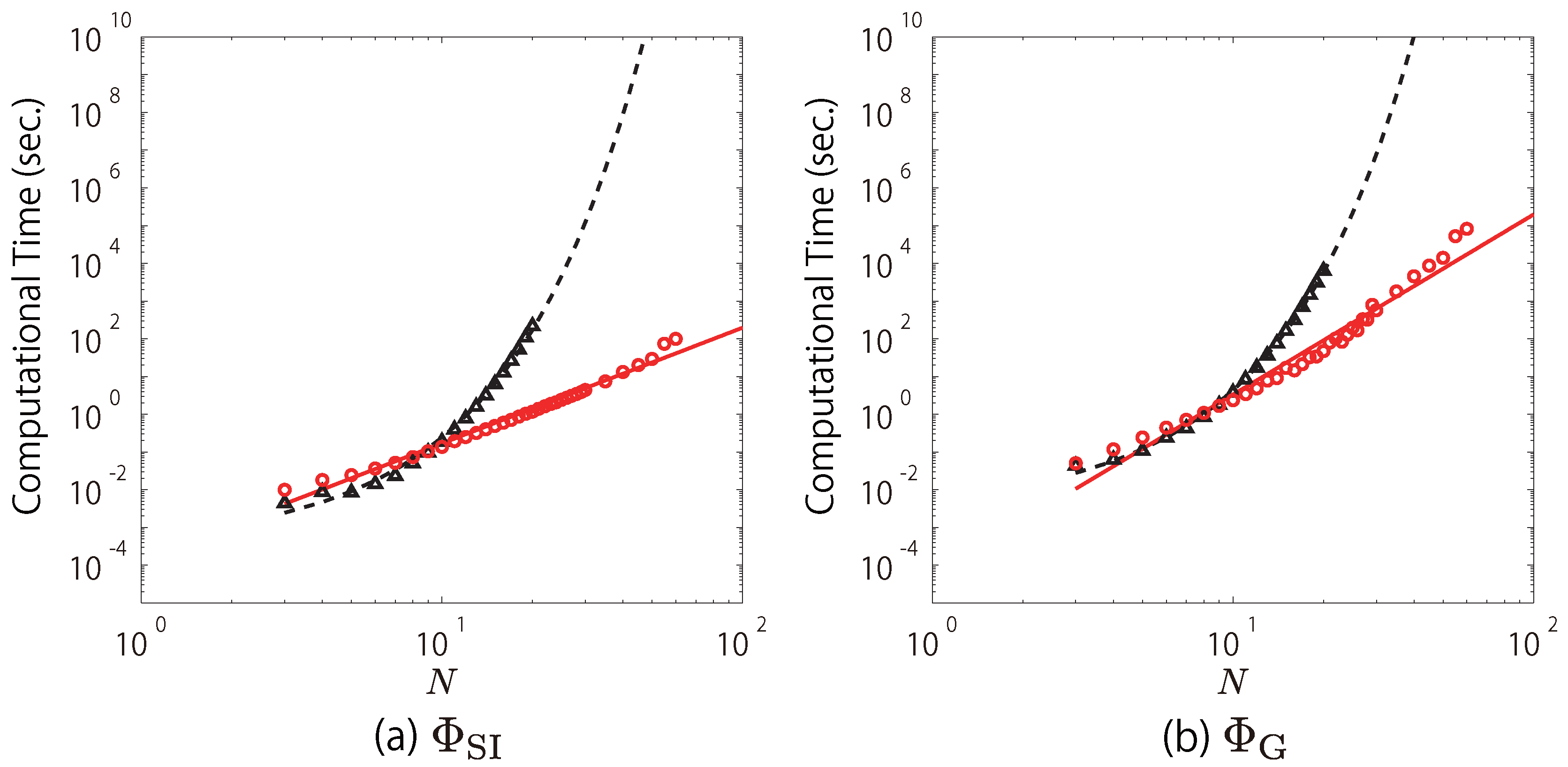
We fitted the computational time of the search using Queyranne’s algorithm for
and
with straight lines, although the computational time for large
N is a little deviated from the straight lines (
Figure 2a,b). In
Figure 2a, the red circles, which indicate the computational time of the search using Queyranne’s algorithm for
, are roughly approximated by the red solid line,
. In contrast, the black triangles, which indicate those of the exhaustive search, are fit by the black dashed line,
. This means that the computational time of the search using Queyranne’s algorithm increases in polynomial order (
), while that of the exhaustive search exponentially increases (
). For example, when
, Queyanne’s algorithm takes ∼197 s while the exhaustive search takes
s. This is in practice impossible to compute even with a supercomputer. Similarly, as shown in
Figure 2b, when
is used, the search using Queyranne’s algorithm roughly takes
while the exhaustive search takes
. Note that the complexity of the search using Queyranne’s algorithm for
(
) is much higher than that of Queyranne’s algorithm itself (
). This is because the multi-dimensional equations (Equations (
A20) and (
A21)) need to be solved by using an iterative method to compute
(see
Appendix A).
6.2. Accuracy of Queyranne’s Algorithm
We evaluated the accuracy of Queyranne’s algorithm by comparing the partition found by Queyranne’s algorithm with the MIP found by exhaustive search. We used and as the measures of integrated information. We considered two different architectures in connectivity matrix A of AR models. The first one was just a random matrix: Each element of A was randomly sampled from a normal distribution with mean 0 and variance . The other one was a block matrix consisting of by sub-matrices, . Each element of diagonal sub-matrices and was drawn from a normal distribution with mean 0 and variance . Off-diagonal sub-matrices and were zero matrices. The covariance of Gaussian noise E in the AR model was generated from a Wishart distribution . The parameter was set to 0.1 or 0.01. The number of elements N was set to 14. We randomly generated 100 connectivity matrices A and for each setting and evaluated performance using the following four measures. The following measures are averaged over 100 trials:
Correct rate (CR): Correct rate (CR) is the rate of correctly finding the MIP.
Rank (RA): Rank (RA) is the rank of the partition found by Queyranne’s algorithm among all possible partitions. The rank is based on the values computed at each partition. The partition that gives the lowest is rank 1. The highest rank is equal to the number of possible bi-partitions, .
Error ratio (ER): Error ratio (ER) is the deviation of the value of integrated information computed across the partition found by Queyranne’s algorithm from that computed across the MIP, which is normalized by the mean error computed at all possible partitions. Error ratio is defined by
where
,
, and
are the amount of integrated information computed across the MIP, that computed across the partition found by Queyranne’s algorithm, and the mean of the amounts of integrated information computed across all possible partitions, respectively.
Correlation (CORR): Correlation (CORR) is the correlation between the partition found by Queyranne’s algorithm and the MIP found by the exhaustive search. Let us represent a bi-partition of
N-elements as an
N-dimensional vector
, where
indicates one of the two subgroups. The absolute value of the correlation between the vector given by the MIP (
) and that given by the partition found by Queyranne’s algorithm (
) is computed:
where
and
are the means of
and
, respectively.
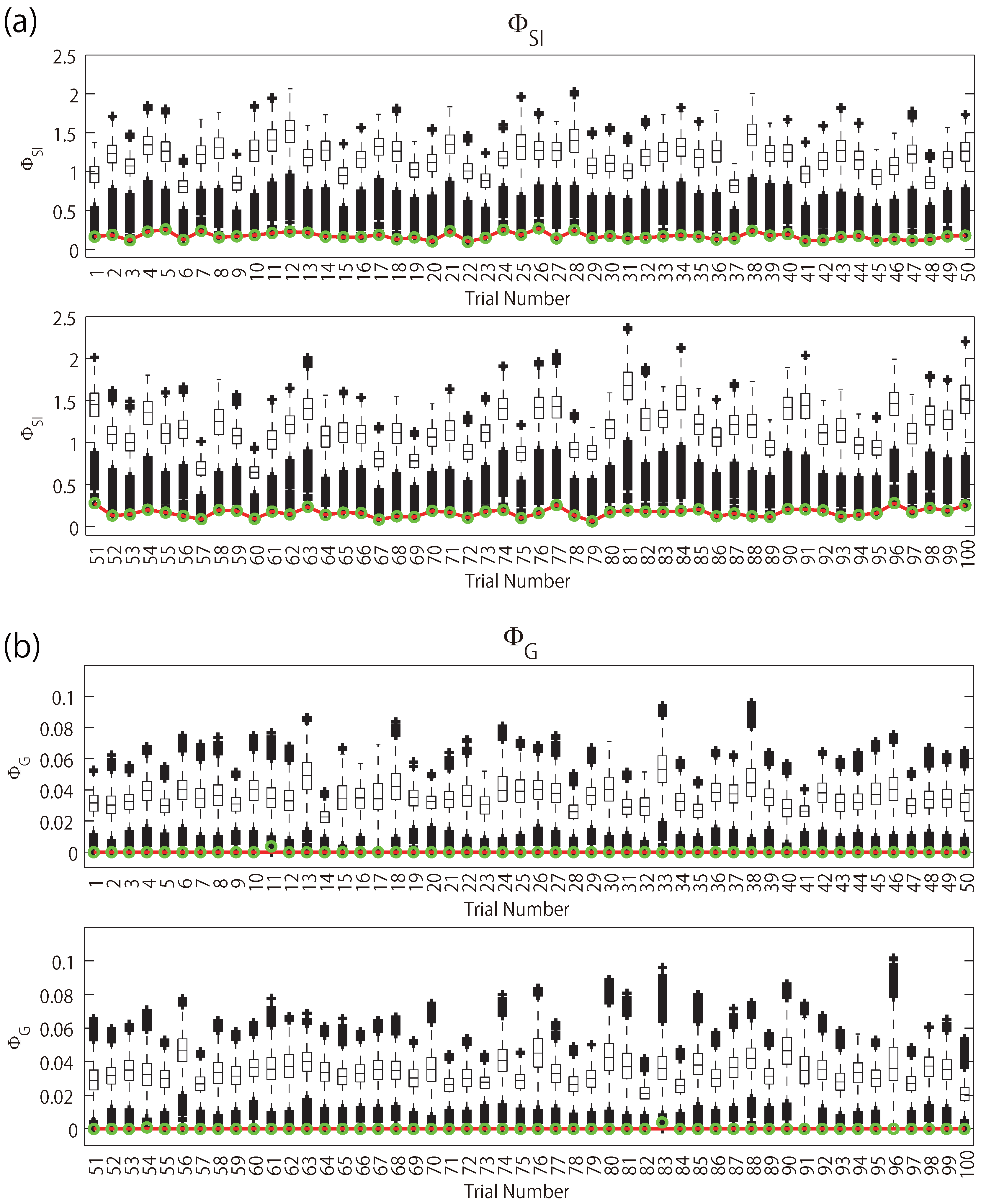
The results are summarized in
Table 1. This table shows that, when
was used, Queyranne’s algorithm perfectly found the MIPs for all 100 trials, even though
is not strictly submodular. Similarly, when
was used, Queyranne’s algorithm almost perfectly found the MIPs. The correct rate was 100% for the normal models and 97% for the block structured models. Additionally, even when the algorithm missed the MIP, the rank of the partition found by the algorithm was 2 or 3. The averaged rank over 100 trials were 1.03 and 1.05 for the block structured models. In addition, the error ratio in error trials were around 0.1 and the average error ratios were very small. See
Appendix C for box plots of the values of the integrated information at all the partitions. Thus, such miss trials would not affect evaluation of the amount of integrated information in practice. However, in terms of partitions, the partitions found by Queyranne’s algorithm in error trials were markedly different from the MIPs. In the block structured model, the MIP for
was the partition that split the system in halves. In contrast, the partitions found by Queyranne’s algorithm were one-vs-all partitions.
In summary, Queyranne’s algorithm perfectly worked for
. With regards to
, although Queyranne’s algorithm almost perfectly evaluated the amount of integrated information, we may need to treat partitions found by the algorithm carefully. This slight difference in performance between
and
can be explained by the order relation in Equation (
13).
is closer to the strictly submodular function
than
is, which we consider to be why Queyranne’s algorithm worked better for
than
.
6.3. Comparison between Queyranne’s Algorithm and REMCMC
We evaluated the performance of Queyranne’s algorithm in large systems where an exhaustive search is impossible. We compared it with the Replica Exchange Markov Chain Monte Carlo Method (REMCMC). We applied the two algorithms to AR models generated similarly as in the previous section. The number of elements was 50 for
and 20 for
, respectively. The reason for the difference in
N is because
requires much heavier computation than
(see
Appendix A). We randomly generated 20 connectivity matrices
A and
for each setting. We compared the two algorithms in terms of the amount of integrated information and the number of evaluations of
. REMCMC was run until a convergence criterion was satisfied. See
Appendix B.3 for details of the convergence criterion.
The results are shown in
Table 2 and
Table 3. “Winning percentage” indicates the fraction of trials each algorithm won in terms of the amount of integrated information at the partition found by each algorithm. We can see that the partitions found by the two algorithms exactly matched for all the trials. We consider that the algorithms probably found the MIPs for the following three reasons. First, it is well known that REMCMC can find a minima if it is run for a sufficiently long time in many applications [
24,
32,
33,
34]. Second, the two algorithms are so different that it is unlikely that they both incorrectly identified the same partitions as the MIPs. Third, Queyranne’s algorithm successfully finds the MIPs in smaller systems as shown in the previous section. This fact suggests that Queyranne’s algorithm worked well also for the larger systems. Note that, in the case of
, the half-and-half partition is the MIP in the block structured model because
under the half-and-half partition. We confirmed that the partitions found by Queyanne’s algorithm and REMCMC were both the half-and-half partition for all the 20 trials. Thus, in the block structured case, it is certain that the true MIPs were successfully found by both algorithms.
We also evaluated the number of evaluations of
in both algorithms before the end of the computational processes. In our simulations, the computational process of Queyranne’s algorithm ended much faster than the convergence of REMCMC. Queyranne’s algorithm ends at a fixed number of evaluations of
depending only on
N. In contrast, the number of the evaluations before the convergence of REMCMC depends on many factors such as the network models, the initial conditions, and pseudo random number sequences. Thus, the time of convergence varies among different trials. Note that, by “retrospectively” examining the sequence of the Monte Carlo search, the solutions turned out to be found at earlier points of the Monte Carlo searches than Queyranne’s algorithm (which are indicated as “solution found” in
Table 2 and
Table 3). However, it is impossible to stop the REMCMC algorithm at these points where the solutions were found because there is no way to tell whether these points reach the solution until the algorithm is run for enough amount of time.
6.4. Evaluation with Real Neural Data
Finally, to ensure the applicability of Queyranne’s algorithm to real neural data, we similarly evaluated the performance with electrocorticography (ECoG) data recorded in a macaque monkey. The dataset is available at an open database, Neurotycho.org (
http://neurotycho.org/) [
35]. One hundred twenty-eight channel ECoG electrodes were implanted in the left hemisphere. The electrodes were placed at 5 mm intervals, covering the frontal, parietal, temporal, and occipital lobes, and medial frontal and parietal walls. Signals were sampled at a rate of 1k Hz and down-sampled to 100 Hz for the analysis. The monkey “Chibi” was awake with the eyes covered by an eye-mask to restrain visual responses. To remove line noise and artifacts, we performed bipolar re-referencing between nearest neighbor electrode pairs. The number of re-referenced electrodes was 64 in total.
In the first simulation, we evaluated the accuracy. We extracted a 1 min length of the signals of the 64 electrodes. Each 1 min sequence consists of 100 Hz × 60 s = 6000 samples. Then, we randomly selected 14 electrodes 100 times. We approximated the probability distribution of the signals with multivariate Gaussian distributions. The covariance matrices were computed with a time window of 1 min and a time step of 10 ms. We applied the algorithms to the 100 randomly selected sets of electrodes and measured the accuracy similarly as in
Section 6.2. The results are summarized in
Table 4. We can see that Queyranne’s algorithm worked perfectly for both
and
.
Next, we compared Queyranne’s algorithm with REMCMC. We applied the two algorithms to the 64 re-referenced signals, and evaluated the performance in terms of the amount of integrated information and the number of evaluations of
, as in
Section 6.3. We segmented 15 non-overlapping sequences of 1 min each, and computed covariance matrices with a time step of 10 ms. We measured the average performance over the 15 sets. Here, we only used
, because
requires heavy computations for 64 dimensional systems. The results are shown in
Table 5. We can see that the partitions selected by the two algorithms matched for all 15 sequences. In terms of the amount of computation, Queyranne’s algorithm ended much faster than the convergence of REMCMC.
7. Discussion
In this study, we proposed an efficient algorithm for searching for the Minimum Information Partition (MIP) in Integrated Information Theory (IIT). The computational time of an exhaustive search for the MIP grows exponentially with the arithmetic growth of system size, which has been an obstacle to applying IIT to experimental data. We showed here that by using a submodular optimization algorithm called Queyranne’s algorithm, the computational time was reduced to and for stochastic interaction and geometric integrated information , respectively. These two measures of integrated information are non-submodular, and thus it is not theoretically guaranteed that Queyranne’s algorithm will find the MIP. We empirically evaluated the accuracy of the algorithm by comparing it with an exhaustive search in simulated data and in ECoG data recorded from monkeys. We found that Queyranne’s algorithm worked perfectly for and almost perfectly for . We also tested the performance of Queyranne’s algorithm in larger systems ( and 50 for and , respectively) where the exhaustive search is intractable by comparing it with the Replica Exchange Markov Chain Monte Carlo method (REMCMC). We found that the partitions found by these two algorithms perfectly matched, which suggests that both algorithms most likely found the MIPs. In terms of the computational time, the number of evaluations of taken by Queyranne’s algorithm was much smaller than that taken by REMCMC before the convergence. Our results indicate that Queyranne’s algorithm can be utilized to effectively estimate MIP even for non-submodular measures of integrated information. Although the MIP is a concept originally proposed in IIT for understanding consciousness, it can be utilized to general network analysis irrespective of consciousness. Thus, the method for searching MIP proposed in this study will be beneficial not only for consciousness studies but for other research fields.
Here, we discuss the pros and cons of Queyranne’s algorithm in comparison with REMCMC. Since the partitions found by both algorithms perfectly matched in our experiments, they were equally good in terms of accuracy. With regards to computational time, Queyranne’s algorithm ended much faster than the convergence of REMCMC. Thus, Queyranne’s algorithm would be a better choice in rather large systems ( and 50 for and , respectively). Note that, if we retrospectively examine the sampling sequence in REMCMC, we find that REMCMC found the partitions much earlier than its convergence and that the estimated MIPs did not change in the later parts of sampling process. Thus, if we could introduce a heuristic criterion to determine when to stop the sampling based on the time course of the estimated MIPs, REMCMC could be stopped earlier than its convergence. However, setting such a heuristic criterion is a non-trivial problem. Queyranne’s algorithm ends within a fixed number of function calls regardless of the properties of data. If the system size is much larger (), Queyranne’s algorithm will be computationally very demanding because of time complexity and may not practically work. In that case, REMCMC would work better if the above-mentioned heuristics are introduced to stop the algorithm earlier than the convergence.
As an alternative interesting approach for approximately finding the MIP, a graph-based algorithm was proposed by Toker and Sommer [
36]. In their method, to reduce the search space, candidate partitions are selected by a spectral clustering method based on correlation. Then
is calculated for those candidate partitions, and the best partition is selected. A difference between our method and theirs is whether the search method is fully based on the values of integrated information or not. Our method uses no other quantities than
for searching the MIP, while their method uses a graph theoretic measure, which may significantly differ from
in some cases. It would be an interesting future work to compare our method and the graph-theoretic methods or combine these methods to develop better search algorithms.
In this study, we considered the three different measures of integrated information,
,
, and
. Of these,
is submodular but the other two measures, while
and
, are not. As we described in
Section 4.3, there is a clear order relation among them (Equation (
13)).
is closer to a submodular function
than
is. This relation implies that Queyranne’s algorithm would work better for
than for
. We found that it was actually the case in our experiments because there were a few error trials for
whereas there were no miss trials for
. For the practical use of these measures, we note that there are two major differences among the three measures. One is what they quantify. As shown in
Figure 1,
measures only causal interactions between units across different time points. In contrast,
and
also measure equal time interactions as well as causal interactions.
best follows the original concept of IIT in the sense that it measures only the “causal” interactions. One needs to acknowledge the theoretical difference whenever applying one of these measures in order to correctly interpret the obtained results. The other difference is in computational costs. The computational costs of
and
are almost the same while that of
is much larger, because it requires multi-dimensional optimization. Thus,
may not be practical for the analysis of large systems. In that case,
or
may be used instead with care taken of the theoretical difference.
Although in this study we focused on bi-partitions, Queyranne’s algorithm can be extended to higher-order partitions [
13]. However, the algorithm becomes computationally demanding for higher-order partitions, because the computational complexity of the algorithm for
K-partitions is
. This is the main reason why we focused on bi-partitions. Another reason is that there has not been an established way to fairly compare partitions with different
K. In IIT 2.0, it was proposed that the integrated information should be normalized by the minimum of the entropy of partitioned subsystems [
3], while, in IIT 3.0, it was not normalized [
4]. Note that, when integrated information is not normalized, the MIP is always found in bi-partitions because integrated information becomes larger when a system is partitioned into more subsystems.
Whether the integrated information should be normalized and how the integrated information should be normalized are still open questions. In our study, the normalization used in IIT 2.0 is not appropriate, because the entropy can be negative for continuous random variables. Additionally, regardless of whether random variables are continuous or discrete, normalization significantly affects the submodularity of the measures of integrated information. For example, if we use normalization proposed in IIT 2.0, even the submodular measure of integrated information, , no longer satisfies submodularity. Thus, Queyranne’s algorithm may not work well if is normalized.
Although we resolved one of the major computational difficulties in IIT, an additional issue still remains. Searching for the MIP is an intermediate step in identifying the informational core, called the “complex”. The complex is the subnetwork in which integrated information is maximized, and is hypothesized to be the locus of consciousness in IIT. Identifying the complex is also represented as a discrete optimization problem which requires exponentially large computational costs. Queyranne’s algorithm cannot be applied to the search for the complex because we cannot formulate it as a submodular optimization. We expect that REMCMC would be efficient in searching for the complex and will investigate its performance in a future study.
An important limitation of this study is that we only showed the nearly perfect performance of Queyranne’s algorithm in limited simulated data and real neural data. In general, we cannot tell whether Queyranne’s algorithm works well for other data beforehand. For real data analysis, we recommend that the procedure below should be applied. First, as we did in
Section 6.2, accuracy should be checked by comparing it with the exhaustive search in small randomly selected subsets. Next, if it works well, the performance should be checked by comparing it with REMCMC in relatively large subsets, as we did in
Section 6.3. If Queyranne’s algorithm works better than or equally as well as REMCMC, it is reasonable to use Queyranne’s algorithm for the analysis. By applying this procedure, we expect that Queyranne’s algorithm could be utilized to efficiently find the MIP in a wide range of time series data.


