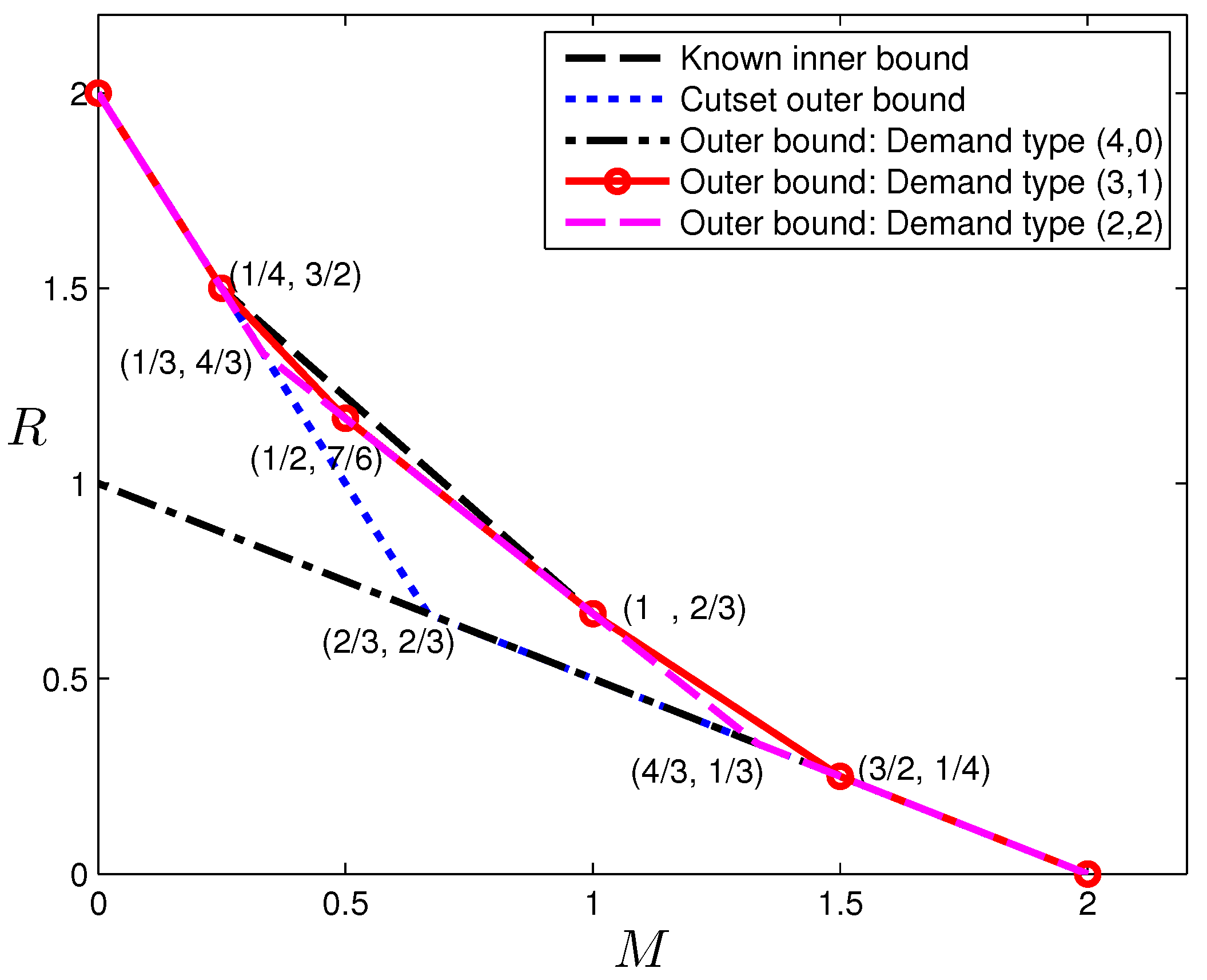
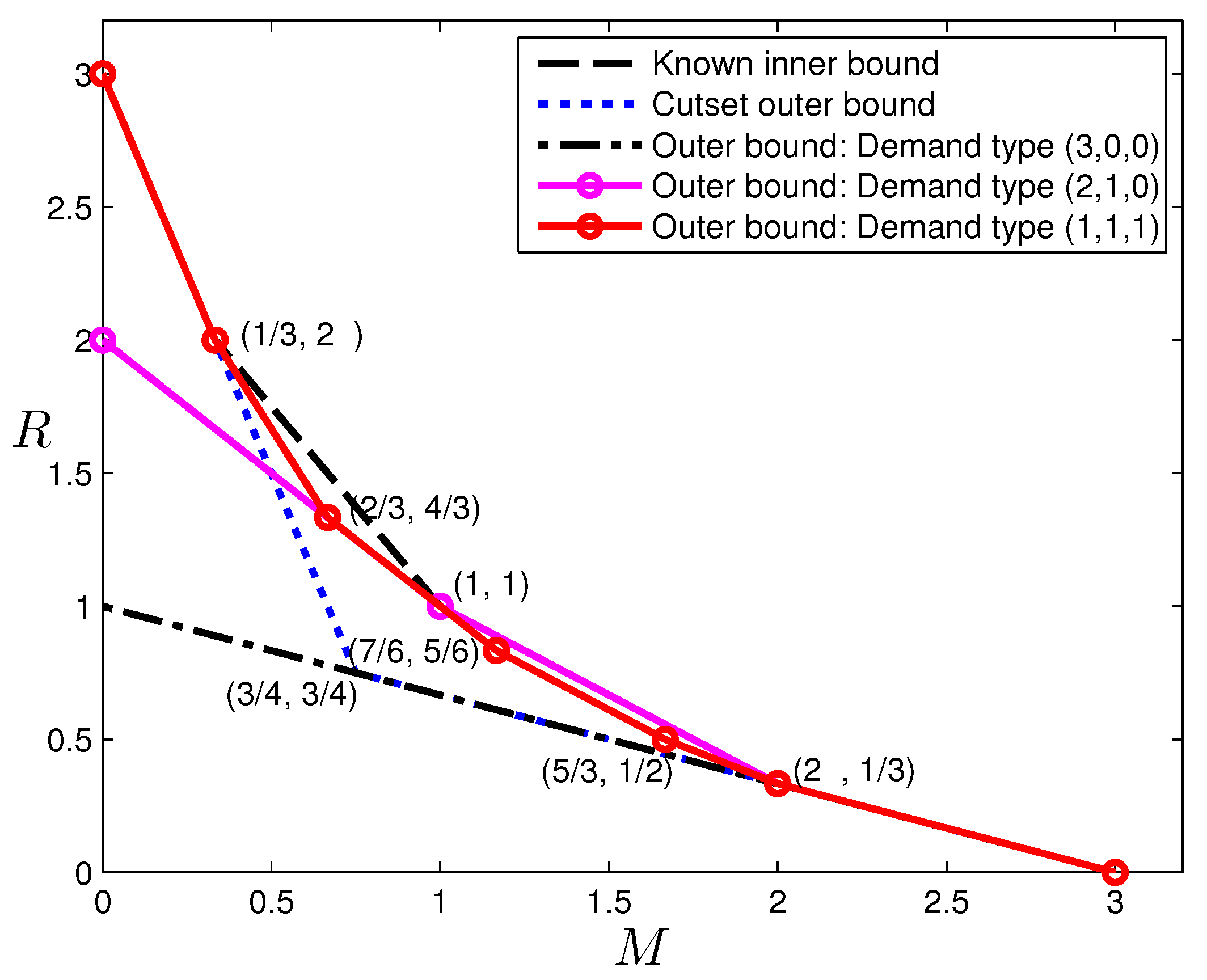
In the previous section, outer bounds of the optimal tradeoff were presented for the case
, which is given in
Figure 3. Observe that the corner points:
cannot be achieved by existing codes in the literature. The former point can indeed be achieved with a new code construction. This construction was first presented in [
20], where it was generalized more systematically to yield a new class of codes for any
, the proof and analysis of which are more involved. In this paper, we focus on how a specific code for this corner point was found through a reverse-engineering approach, which should help dispel the mystery on this seemingly arbitrary code construction.
5.2. Extracting Information for Reverse-Engineering
It is clear at this point that for this case of , the code to achieve this optimal corner point is not straightforward. Next, we discuss a general approach to deduce the code structure from the LP solution, which leads to the discovery of the code in our work. The approach is based on the following assumptions: the outer bound is achievable (i.e., tight); moreover, there is a (vector) linear code that can achieve this performance.
Either of the two assumptions above may not hold in general, and in such a case, our attempt will not be successful. Nevertheless, though linear codes are known to be insufficient for all network coding problems [
33], existing results in the literature suggest that vector linear codes are surprisingly versatile and powerful. Similarly, though it is known that Shannon-type inequalities, which are the basis for the outer bounds computation, are not sufficient to characterize rate region for all coding problems [
34,
35], they are surprisingly powerful, particularly in coding problems with strong symmetry structures [
36,
37].
There are essentially two types of information that we can extract from the primal LP and dual LP:
From the effective information inequalities: since we can produce a readable proof using the dual LP, if a code can achieve this corner point, then the information inequalities in the proof must hold with equality for the joint entropy values induced by this code, which reveals a set of conditional independence relations among random variables induced by this code;
From the extremal joint entropy values at the corner points: although we are only interested in the tradeoff between the memory and transmission rate, the LP solution can provide the whole set of joint entropy values at an extreme point. These values can reveal a set of dependence relations among the random variables induced by any code that can achieve this point.
Though the first type of information is important, its translation to code constructions appears difficult. On the other hand, the second type of information appears to be more suitable for the purpose of code design, which we adopt next.
One issue that complicates our task is that the entropy values so extracted are not always unique, and sometimes have considerable slacks. For example, for different LP solutions at the same operating point of
, the joint entropy
can vary between one and
. We can identify such a slack in any joint entropy in the corner point solutions by considering a regularized primal LP: for a fixed rate value
R at the corner point in question as an upper bound, the objective function can be set as:
instead of:
subject to the same original symmetric LP constraints at the target
M. By choosing a small positive γ value, e.g.,
, we can find the minimum value for
at the same
point; similarly, by choosing a small negative γ value, we can find the maximum value for
at the same
point. Such slacks in the solution add uncertainty to the codes we seek to find and may indeed imply the existence of multiple code constructions. For the purpose of reverse-engineering the codes, we focus on the joint entropies that do not have any slacks, i.e., the “stable” joint entropies in the solution.
5.3. Reverse-Engineering the Code for
With the method outlined above, we identify the following stable joint entropy values in the
case for the operating point
listed in
Table 3. The values are normalized by multiplying everything by six. For simplicity, let us assume that each file has six units of information, written as
and
, respectively. This is a rich set of data, but a few immediate observations are given next.
The quantities can be categorized into three groups: the first is without any transmission; the second is the quantities involving the transmission to fulfill the demand type ; and the last for demand type .
The three quantities and provide the first important clue. The values indicate that for each of the two files, each user should have three units in his/her cache, and the combination of any two users should have five units in their cache, while the combination of any three users should have all six units in their cache. This strongly suggests placing each piece (and ) at two users. Since each has four units, but it needs to hold three units from each of the two files, coded placement (cross files) is thus needed. At this point, we place the corresponding symbols in the caching, but keep the precise linear combination coefficients as undetermined.
The next critical observation is that . This implies that the transmission has three units of information on each file alone. However, since the operating point dictates that , it further implies that in each transmission, three units are for the linear combinations of , and 3 units are for those of ; in other words, the linear combinations do not need to mix information from different files.
Since each transmission only has three units of information from each file, and each user has only three units of information from each file, they must be linearly independent of each other.
The observation and deductions are only from the perspective of the joint entropies given in
Table 3, without much consideration of the particular coding requirement. For example, in the last item discussed above, it is clear that when transmitting the three units of information regarding a file (say file
), they should be simultaneously useful to other users requesting this file, and to the users not requesting this file. This intuition then strongly suggests each transmitted linear combination of
should be a subspace of the
parts at some users not requesting it. Using these intuitions as guidance, finding the code becomes straightforward after trial-and-error. In [
20], we were able to further generalize this special code to a class of codes for any case when
; readers are referred to [
20] for more details on these codes.
5.4. Disproving Linear-Coding Achievability
The reverse engineering approach may not always be successful, either because the structure revealed by the data is very difficult to construct explicitly, or because linear codes are not sufficient to achieve this operating point. In some other cases, the determination can be done explicitly. In the sequel, we present an example for , which belongs to the latter case. An outer bound for is presented in the next section, and among the corner points, the pair is the only one that cannot be achieved by existing schemes. Since the outer bound appears quite strong, we may conjecture this pair to be also achievable and attempt to construct a code. Unfortunately, as we shall show next, there does not exist such a (vector) linear code. Before delving into the data provided by the LP, readers are encouraged to consider proving directly that this tradeoff point cannot be achieved by linear codes, which does not appear to be straightforward to the author.
We shall assume each file has
symbols in a certain finite field, where
m is a positive integer. The LP produces the joint entropy values (in terms of the number of finite field symbols, not in multiples of file size as in the other sections of the paper) in
Table 4 at this corner point, where only the conditional joint entropies relevant to our discussion next are listed. The main idea is to use these joint entropy values to deduce structures of the coding matrices, and then combining these structures with the coding requirements to reach a contradiction.
The first critical observation is that
, and the user-index-symmetry implies that
. Moreover
, from which we can conclude that excluding file
and
, each user stores
m linearly independent combinations of the symbols of file
, which are also linearly independent among the three users. Similar conclusions hold for files
and
. Thus, without loss of generality, we can view the linear combinations of
cached by the users, after excluding the symbols from the other two files, as the basis of file
. In other words, this implies that through a change of basis for each file, we can assume without loss of generality that user
k stores
linear combinations in the following form:
where
is the j-th symbol of the n-th file and
is a matrix of dimension
;
can be partitioned into submatrices of dimension
, which are denoted as
,
and
. Note that symbols at different users are orthogonal to each other without loss of generality.
Without loss of generality, assume the transmitted content
is:
where
G is a matrix of dimension
; we can partition it into blocks of
, and each block is referred to as
,
and
. Let us first consider User 1, which has the following symbols:
The coding requirement states that
and
together can be used to recover file
, and thus, one can recover all the symbols of
knowing (
45). Since
can be recovered, its symbols can be eliminated in (
45), i.e.,
in fact becomes known. Notice
Table 4 specifies
, and thus, the matrix:
is in fact full rank; thus, from the top part of (
46),
and
can be recovered. In summary, through elemental row operations and column permutations, the matrix in (
45) can be converted into the following form:
where diagonal block square matrices are of full rank
and
, respectively, and
’s are the resultant block matrices after the row operations and column permutations. This further implies that the matrix
has maximum rank
m. and it follows that the matrix:
i.e., the submatrix of
G by taking thick columns
has only maximum rank
m. However, due to the symmetry, we can also conclude that the submatrix of
G taking only thick columns
and that taking only thick columns
both have only maximum rank
m. As a consequence, the matrix
G has rank no larger than
, but this contradicts the condition that
in
Table 4. We can now conclude that this memory-transmission-rate pair is not achievable with any linear codes.
Strictly speaking, our argument above holds under the assumption that the joint entropy values produced by LP are precise rational values, and the machine precision issue has thus been ignored. However, if the solution is accurate only up to machine precision, one can introduce a small slack value δ into the quantities, e.g., replacing with , and using a similar argument show that the same conclusion holds. This extended argument however becomes notationally rather lengthy, and we thus omitted it here for simplicity.


