Abstract
The statistical properties of chaotic binary sequences generated by the Bernoulli map and Walsh functions are discussed. The Walsh functions are based on a Hadamard matrix. For general k (=), we will prove that Walsh functions can generate essentially different balanced and i.i.d. binary sequences that are orthogonal to each other.
1. Introduction
The simplest way to generate chaos is to use a one-dimensional(1D) nonlinear difference equation with a chaotic map. Chaotic sequences can be used as random numbers for several engineering applications, and there have been many works on chaos-based random number generation [1,2,3,4,5,6,7,8,9,10,11]. In general, truly random numbers should be a sequence of i.i.d. (independent and identically distributed) random variables with a uniform probability density, that is they give maximum entropy. Their typical model, for example, is a sequence obtained by trials of fair coin-tossing or dice-throwing. The design of many chaotic sequences of i.i.d. binary (or p-ary) random variables from a single chaotic real-valued sequence generated by a class of 1D nonlinear maps was established in [1,2,3], where it was shown that some symmetric binary (or p-ary) functions can produce i.i.d. binary (or p-ary) sequences if the map satisfies some symmetric properties.
In some engineering applications (e.g., communication, cryptography, the Monte Carlo method) of chaos-based random numbers, their statistical properties such as distributions and correlations are very important. Whereas there are some indices for defining chaos such as Lyapunov exponents, we concentrate on statistical properties in this paper. Thus, we discuss the statistical properties of orthogonal chaotic binary sequences generated by the Bernoulli map and Walsh functions based on Hadamard matrices, which was already discussed in [12]. As is well known, Walsh functions are the most famous orthogonal binary functions, and they can be applied to many applications (e.g., signal processing) [13,14,15,16,17]. In [12], we proved that the Bernoulli map and Walsh functions based on the () Hadamard matrix can generate different balanced i.i.d. binary sequences that are orthogonal to each other. Here, “balanced” means that the probability of “1” (or “0”) in the binary sequence is equal to 1/2. We conjectured that this holds for general positive integers k. In this paper, we will give a rigorous proof of this for general k.
2. Preliminaries
For a nonlinear map , a chaotic sequence can be generated by a 1D difference equation:
where and is called an initial value or a seed. For an integrable function G, the average (expectation) of a sequence is defined by:
which is very important in evaluating the statistics of chaotic sequences under the assumption that is mixing on I with respect to an absolutely continuous invariant measure, denoted by .
Definition 1.
For two chaotic sequences and generated from a common seed x, their cross-correlation function is defined by:
where ℓ is a time shift. If , the two sequences and are called uncorrelated or orthogonal to each other. Note that is the auto-correlation function of .
Definition 2.
The Perron-Frobenius (PF) operator of the map τ with an interval is defined by:
which can be rewritten as:
where is the i-th preimage of the map [18].
Remark 1.
The PF operator given in Definition 2 is very useful for evaluating correlation functions because it has the following important property [18]:
Remark 3.
For a binary function (), a sufficient condition for a binary sequence to be i.i.d. is given by [1]:
which can also be expressed as:
3. Hadamard Matrix and Walsh Functions
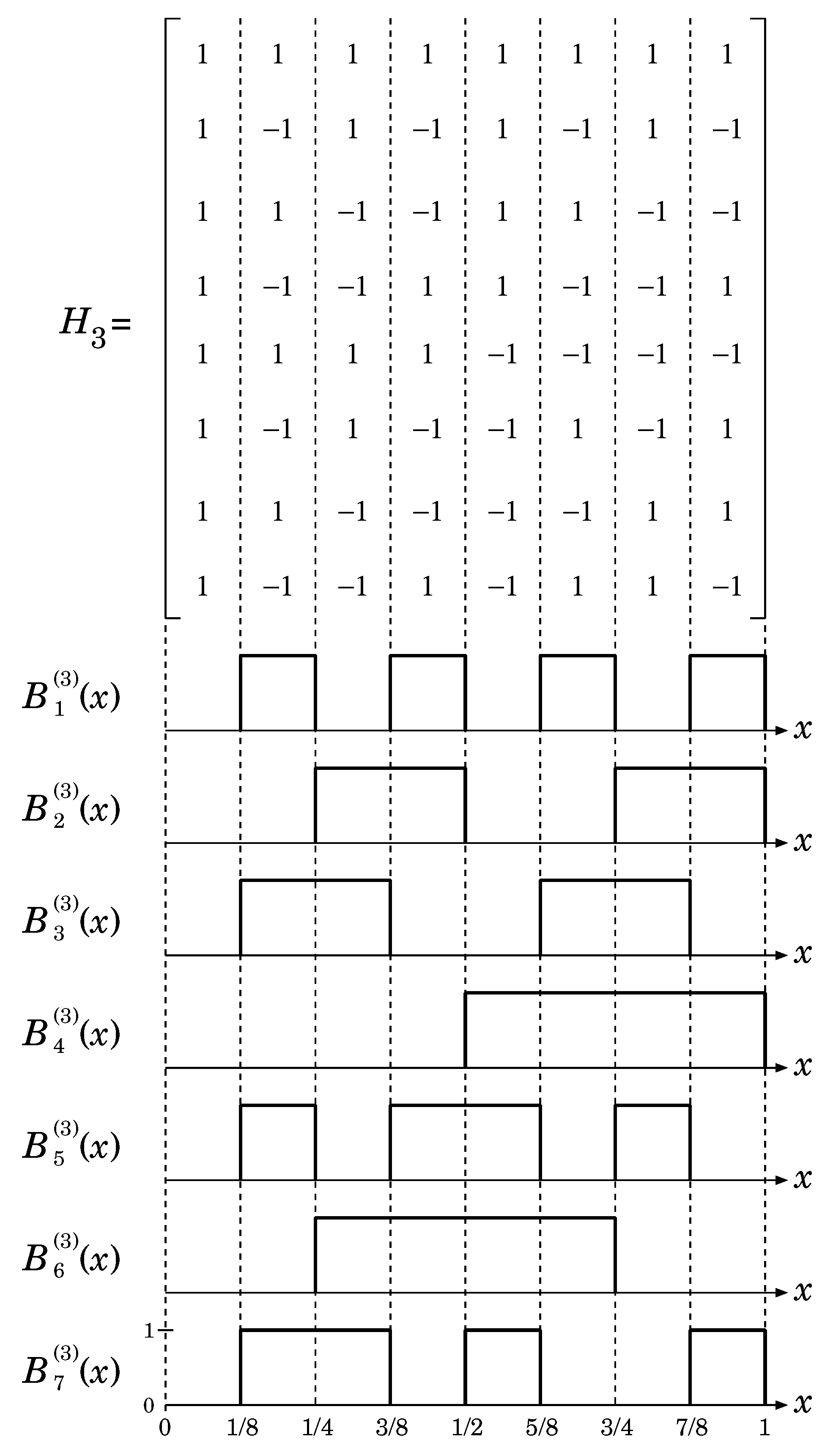
We introduce a Hadamard matrix defined by [13,14,15]:
which is one of the orthogonal matrices whose rows (or columns) are orthogonal -tuples. For example, is given by:
Furthermore, can be expressed as:
where ⊗ denotes the Kronecker product.
Denote the -th element of by . Then, we consider binary functions () defined by:
As an example, () are shown in Figure 1. Note that () correspond to Walsh functions in natural (Hadamard) order, which include Rademacher functions [13,14].
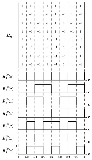
Figure 1.
Binary (Walsh) functions based on an Hadamard matrix ().
Proposition 1.
The following relation:
is satisfied. Namely, () include all of ().
Proof.
This completes the proof. □
4. Orthogonal Chaotic Binary Sequences
For chaotic binary sequences () generated by a nonlinear map with and , it is obvious that:
that is, the binary sequences are balanced. Note that is excluded here since . Furthermore, we have:
which gives:
This implies that the binary sequences are orthogonal to each other.
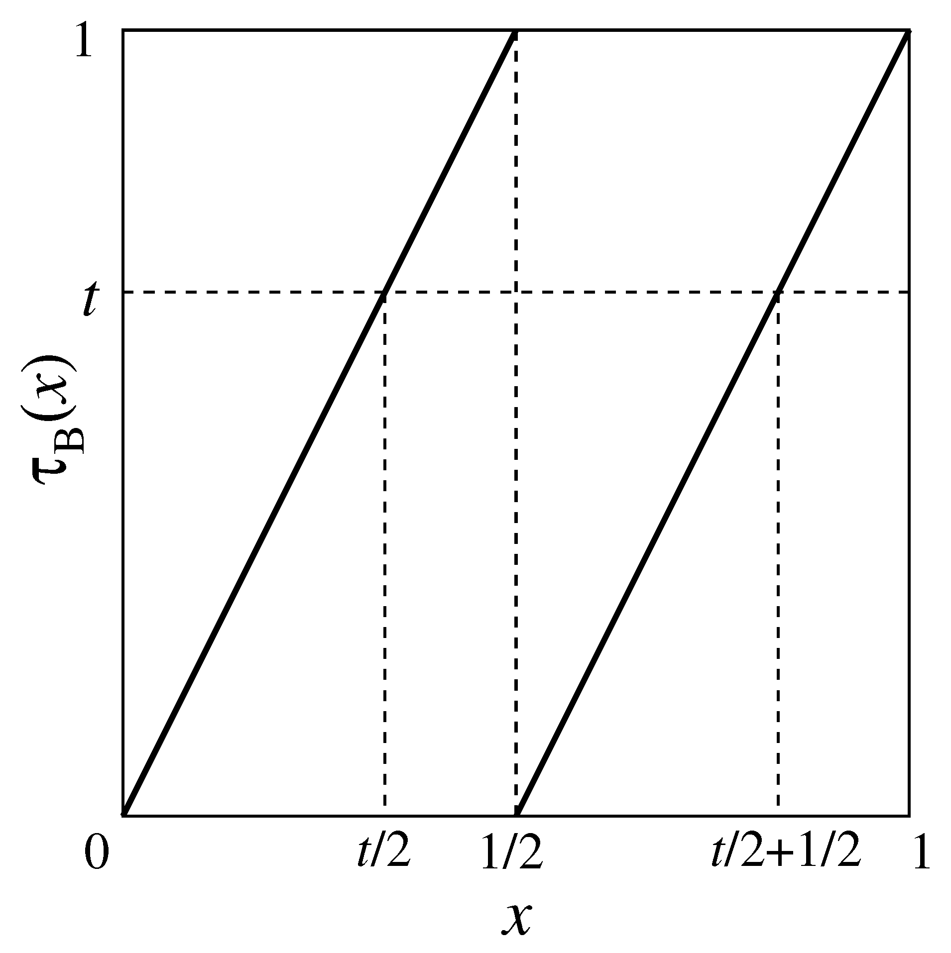
In this paper, we employ Bernoulli map defined by:
which has the uniform invariant density for the unit interval . Figure 2 shows the map.
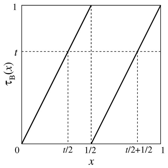
Figure 2.
Bernoulli map.
Proposition 2.
For Walsh functions and Bernoulli map , the following relation:
is satisfied.
Proof.
Remark 4.
From Propositions 1 and 2, we have:
which implies that some of the binary sequences () are time-shifted versions of others.
Theorem 1.
For Bernoulli map , we have:
Proof.
Remark 5.

From Remarks 2 and 3 and the above Theorem, each of binary sequences is a balanced i.i.d. binary sequence, and they are uncorrelated (orthogonal) with each other for any time shift ℓ including , that is we have:
It should be noted that Equation (34) implies that binary sequences () are essentially different, that is they are not time-shifted versions of the others. Table 1 shows the evaluation results for the case .
Table 1.
Evaluation results for the case .
5. Conclusions
We theoretically evaluated the statistical properties of chaotic binary sequences generated by the Bernoulli map and Walsh functions. For given k, it was shown that binary sequences are essentially different in the sense that none of them are time-shifted versions of the others. Furthermore, we showed that each of the binary sequences is a balanced i.i.d. sequence, and they are uncorrelated (orthogonal) with each other for any time shift.
As in [12,19], the Bernoulli map can be approximated by nonlinear feedback shift registers (NFSRs) [20] with finite bits, and the binary functions corresponding to can be easily realized by combinational logic circuits. We will discuss the applications of the orthogonal binary sequences using such NFSRs in our future study.
Funding
This work was supported by JSPS KAKENHI Grant Number JP16K06361 and JP19K12158.
Conflicts of Interest
The author declares no conflict of interest.
References
- Kohda, T.; Tsuneda, A. Statistics of chaotic binary sequences. IEEE Trans. Inf. Theory 1997, 43, 104–112. [Google Scholar] [CrossRef]
- Kohda, T.; Tsuneda, A. Design of sequences of i.i.d. p-ary random variables. In Proceedings of the 1997 IEEE International Symposium on Information Theory, Ulm, Germany, 6–7 July 1997; p. 17. [Google Scholar]
- Kennedy, M.; Setti, G.; Rovatti, R. Chaotic Electronics in Telecommunications; CRC Press: New York, NY, USA, 2000. [Google Scholar]
- Stojanovski, T.; Kocarev, L. Chaos-based random number generators—Part I: analysis. IEEE Trans. Circuits Syst. I 2001, 48, 281–288. [Google Scholar] [CrossRef]
- Stojanovski, T.; Pihl, J.; Kocarev, L. Chaos-based random umber generators—Part II: practical realization. IEEE Trans. Circuits Syst. I 2001, 48, 382–385. [Google Scholar] [CrossRef]
- Bernardini, R.; Cortelazzo, G. Tools for designing chaotic systems for secure random number generation. IEEE Trans. Circuits Syst. I 2001, 48, 552–564. [Google Scholar] [CrossRef]
- Gerosa, A.; Bernardini, R.; Pietri, S. A fully integrated chaotic system for the generation of truly random numbers. IEEE Trans. Circuits Syst. I 2001, 49, 993–1000. [Google Scholar] [CrossRef]
- Fort, A.; Cortigiani, F.; Rocchi, S.; Vignoli, V. Very high-speed true random noise generator. Analog Integr. Circuits Process. 2003, 34, 97–105. [Google Scholar] [CrossRef]
- Kyaw, T.N.N.; Tsuneda, A. Generation of chaos-based random bit sequences with prescribed auto-correlations by post-processing using linear feedback shift registers. NOLTA 2017, 8, 224–234. [Google Scholar] [CrossRef]
- Demir, K.; Ergün, S. An analysis of deterministic chaos as an entropy source for random number generators. Entropy 2018, 20, 957. [Google Scholar] [CrossRef]
- Li, C.; Feng, B.; Li, S.; Kurths, J.; Chen, G. Dynamic analysis of digital chaotic maps via state-mapping networks. IEEE Trans. Circuits Syst. I 2019, 66, 2322–2335. [Google Scholar] [CrossRef]
- Tsuneda, A. Orthogonal chaotic binary sequences based on Walsh functions. In Proceedings of the Second International Workshop on Sequence Design and Its Applications in Communications, Shimonoseki, Japan, 10–14 October 2005. [Google Scholar]
- Beauchamp, K.G. Walsh Functions and Their Applications; Academic Press: Cambridge, MA, USA, 1975. [Google Scholar]
- Davies, A.C. On the definition and generation of Walsh functions. IEEE Trans. Comput. 1972, 100, 187–189. [Google Scholar] [CrossRef]
- Geadah, Y.A.; Corinthios, M.J.G. Natural, dyadic, and sequency order algorithms and processors for the Walsh-Hadamard transform. IEEE Trans. Comput. 1977, C-26, 435–442. [Google Scholar] [CrossRef]
- Golubov, B.; Efimov, A.; Skvortsov, V. Walsh Series and Transforms; Springer: Berlin/Heidelberger, Germany, 1991. [Google Scholar]
- Wang, X.; Liang, X.; Zheng, J.; Zhou, H. Fast detection and segmentation of partial image blur based on discrete Walsh-Hadamard transform. Signal Process.-Image Commun. 2019, 70, 47–56. [Google Scholar] [CrossRef]
- Lasota, A.; Mackey, M.C. Chaos, Fractals, and Noise; Springer: Berlin/Heidelberger, Germany, 1994. [Google Scholar]
- Tsuneda, A.; Kuga, Y.; Inoue, T. New maximal-period sequences using extended nonlinear feedback shift registers based on chaotic maps. IEICE Trans. Fundamentals 2001, E85-A, 1327–1332. [Google Scholar]
- Golomb, S.W. Shift Register Sequences; revised ed.; Aegean Park Press: Laguna Hills, CA, USA, 1982. [Google Scholar]
© 2019 by the author. Licensee MDPI, Basel, Switzerland. This article is an open access article distributed under the terms and conditions of the Creative Commons Attribution (CC BY) license (http://creativecommons.org/licenses/by/4.0/).