3.1. Operation of Joint Detection and Decoding
We consider an iterative JDD process employing a low-complexity detection algorithm based on FG-GAI BP [
22] and a sum-product decoding algorithm. One JDD iteration is composed of
detection iterations followed by
decoding iterations, where we call a JDD iteration as a global iteration. Let us consider the
lth channel use. Then, Equation (
2) can be written as
Each observation node
obtains the information of
,
, from
by regarding terms associated with
,
, as interferences. For this purpose, we define
as the interference plus noise when detecting the symbol
and rewrite Equation (
3) as
In the case of using a massive number of transmit antennas, we can approximate
as a Gaussian random variable [
22] with the mean
and the variance
, where
and
The likelihood of
at each observation node
is approximately obtained by using the Gaussian approximation of
as
where
. Note that
and
are computed as
and
where
denotes a priori probability of
at the observation node
. The extrinsic probability of
at each observation node
is obtained as [
22]
where
is a constant. As simple notations, we let
and
denote the likelihood and the extrinsic probability, respectively, of
at the observation node
, i.e.,
and
.
In the iterative process, the extrinsic probability replaces the role of a priori probability. In other words,
in Equations (
8) and (
9) are replaced by
. Then,
is computed at the observation node
by using
,
, via
and
based on Equations (
7)–(
9) and delivered to the middle node
. Note that
is computed at the middle node
by using
,
, as in Equation (
10), and delivered to the observation node
. Consequently,
and
are updated in a recursive manner through detection iterations.
At the end of detection iterations, the log-likelihood ratios (LLR) of coded bits are computed at middle nodes in the following manner and delivered to the decoder. We suppose that a variable node
represents the
tth bit in the bit-stream generating
, which results in
. Then, the LLR of the coded bit
corresponding to the variable node
is defined by
and obtained at the middle node
as [
22]
where
is the
tth bit of a bit-stream generating a symbol
s is
and
is the
tth bit of a bit-stream generating a symbol
s is
. In the last equality of Equation (
11), we use
. The messages
obtained at middle nodes are delivered to the decoder to be used in the sum-product decoding.
Next, consider the operation of sum-product decoding. Let
and
denote the message flowing from the variable node
to the check node
c and the message flowing from the check node
c to the variable node
, respectively. These messages are updated in an iterative manner by [
29,
30]
and
where
. Note that
denotes the set of check nodes except
c connected to the variable node
and
denotes the set of variable nodes except
connected to the check node
c. At the end of decoding iterations, the LLR message of the
tth bit in the bit-stream generating
is computed as
and delivered to the middle node
in the detector. At the beginning of the next detection iteration, the probability
is computed at the middle node
by
and used in the detector as in Equation (
10), where
denotes the value of the
tth bit in the bit-stream generating a symbol
s.
After
global iterations, the decision on bits is made such that the coded bit
is estimated as 1 if
and as 0 otherwise, where
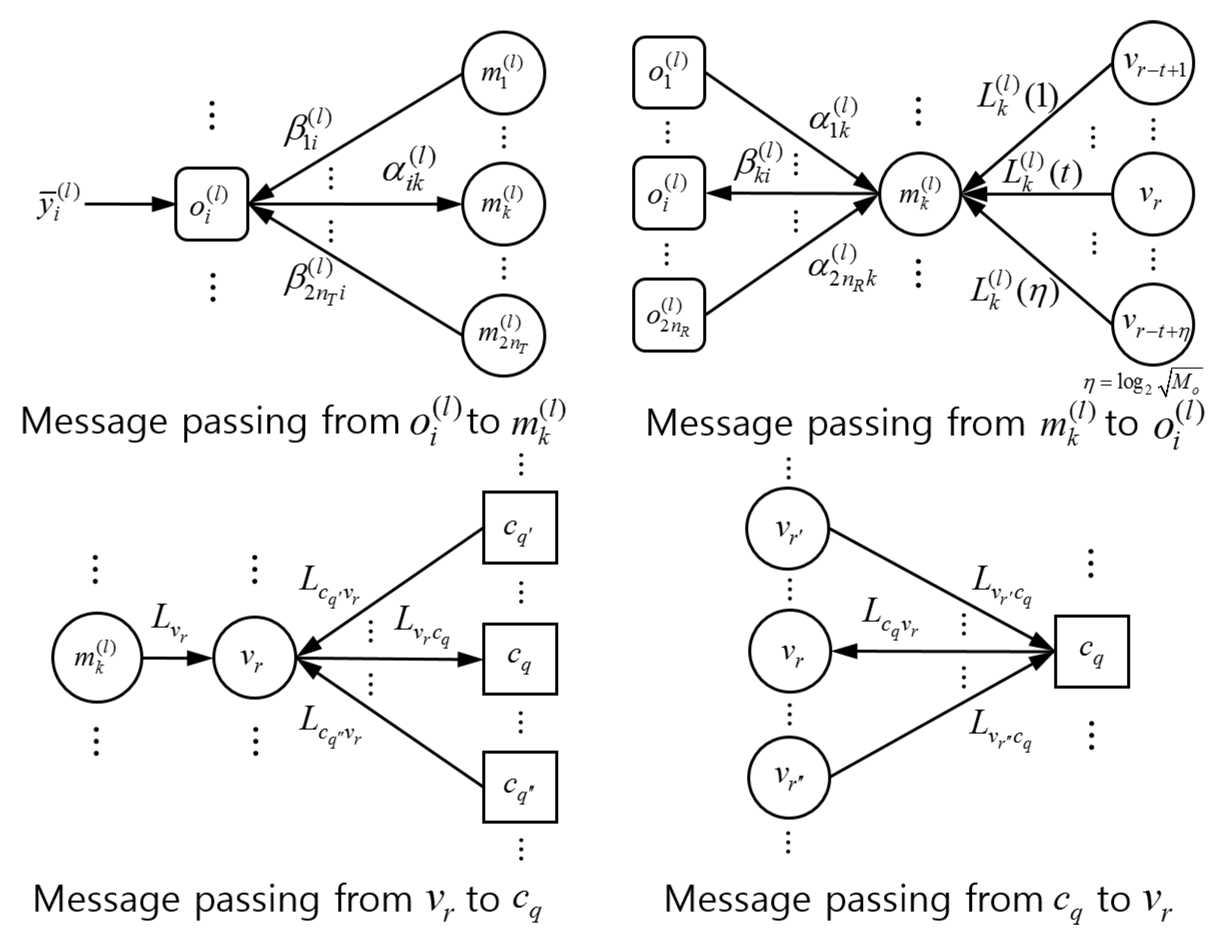
. The overall procedure of JDD is presented in Algorithm 1 and the FG-GAI BP detection is summarized in Algorithm 2. Message flows between component nodes of the JDD are illustrated in
Figure 2.
| Algorithm 1: Joint Detection and Decoding (JDD). |
![Entropy 21 00231 i001]() |
| Algorithm 2: FG-GAI BP detection. |
![Entropy 21 00231 i002]() |
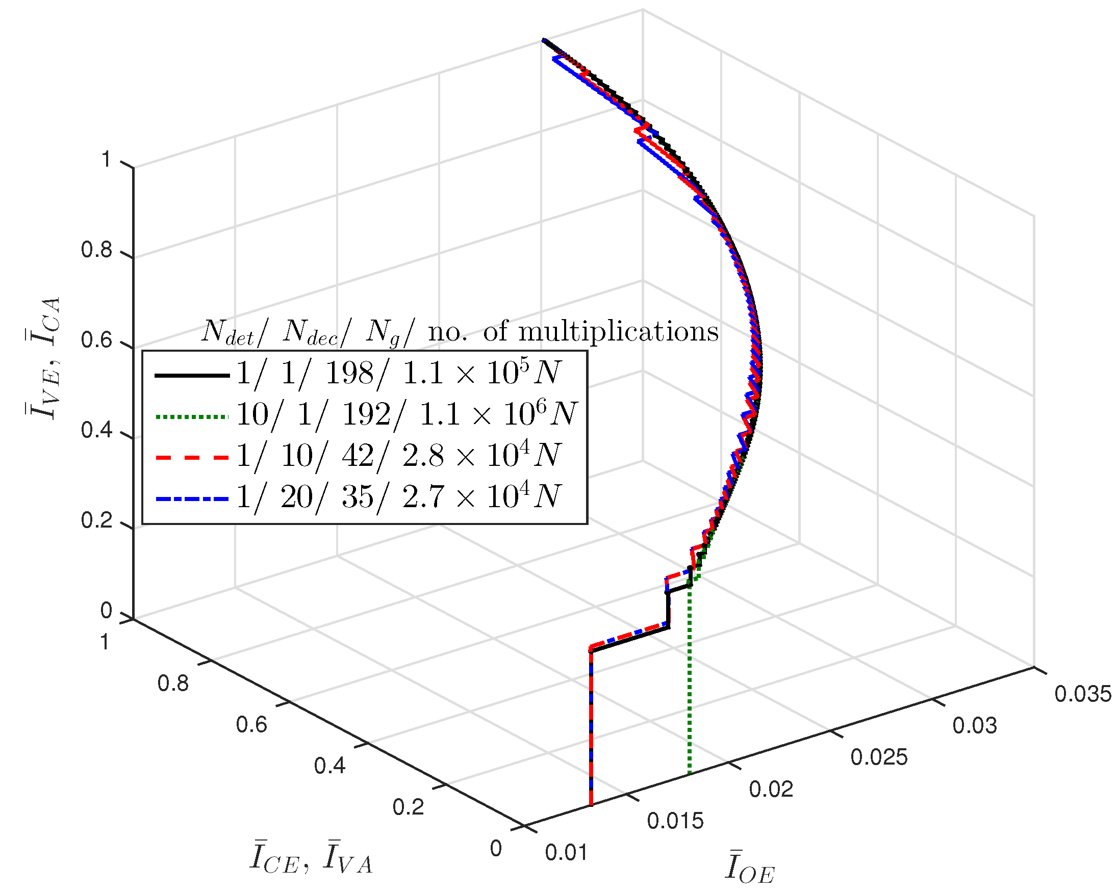
Let us think about the computational complexity of FG-GAI BP detection in terms of the number of multiplications. We focus on one detection iteration for one channel use with a given modulation. It is easily inferred from Algorithm 2 that the FG-GAI BP detection requires a computational complexity of
. For a brief comparison, we consider some other SISO MIMO detectors such as BP detector [
21], SISO MMSE detector, tree-searching detector such as sphere decoding (SD) aided max-log method [
26] and subspace marginalization with interference suppression (SUMIS) detector [
26]. These detectors require computational complexities of
. It is clear that the FG-GAI-BP detector requires lower computational complexity than other SISO MIMO detectors under comparison.
3.2. Analysis of Joint Detection and Decoding
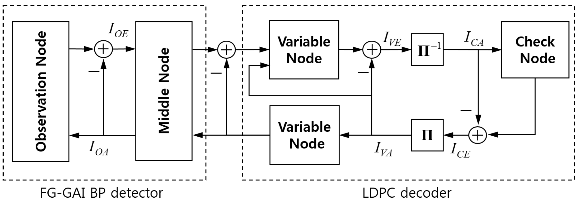
We analyze the behavior of JDD in the receiver of coded massive MIMO system in terms of mutual information transfer characteristics, so-called EXIT characteristics, in component units. We focus on the mutual information between coded bits generating transmit symbols and corresponding message variables. In fact,
and
at the observation node
contain information regarding the transmit symbol
. Thus, for the bit-level EXIT analysis mentioned above, we define new LLR messages of coded bits at observation nodes. Let us consider the
tth bit of a coded bit-stream mapped to
and define two LLR messages of this bit at the observation node
. The first LLR is
sent from
to
, and the second LLR is
sent from
to
, where
. We let
and
denote random variables representing
and
, respectively, for all
, and let
U denote the corresponding coded bit. We suppose all LLR messages are independent and normally distributed. For each observation node, we define
and
. We define
and
at variable nodes, where
and
are incoming and outgoing messages at variable nodes, respectively. We also define
and
at check nodes, where
and
are incoming and outgoing messages at check nodes, respectively. Allowing slight abuse of notation, we use
and
to denote the mutual information between
U and
delivered from degree-
check nodes to a variable node. We also use
and
to denote the mutual information between
U and
delivered from degree-
variable nodes to a check node. We depict the resultant iterative JDD process represented by transfer blocks of mutual information as in
Figure 3.
Consider a degree-
variable node that is connected to
check nodes and
observation nodes via a corresponding middle node. The variable node sums up all incoming messages except one from a target node and sends the result to the target node. Thus,
is obtained by summing up
copies of
and
copies of
. It follows that the variance of
is obtained by adding the variance of
multiplied by
and the variance of
multiplied by
. By defining
as [
33]
we obtain
, where
is the variance of a normally distributed random variable
X. Then,
is obtained as a function of
as
where
is the average of
over
,
denotes the fraction of edges that are connected to check nodes of degree
, and
denotes the maximum degree of check node. Let us define the EXIT function between
and
as
where
is also a function of
due to the dependency of
on
. Note that
is obtained by Monte Carlo simulation [
33]. The LLR message
sent from the variable node to check nodes is obtained by summing up
copies of
and
copies of
. Then, the variance of
is obtained by adding the variance of
multiplied by
and the variance of
multiplied by
. It follows that
In the case of irregular distribution of
, we define averages of
and
over
as
and
respectively, where
denotes the fraction of edges that are connected to variable nodes of degree
and
denotes the maximum degree of variable node.
Let us consider a degree-
check node and define the EXIT function from
to
as [
33]
where
is the average of
over
. In the case of irregular distribution of
, we define the average of
over
as
The density evolution of messages flowing in the JDD process in terms of EXIT characteristics is summarized in Algorithm 3.
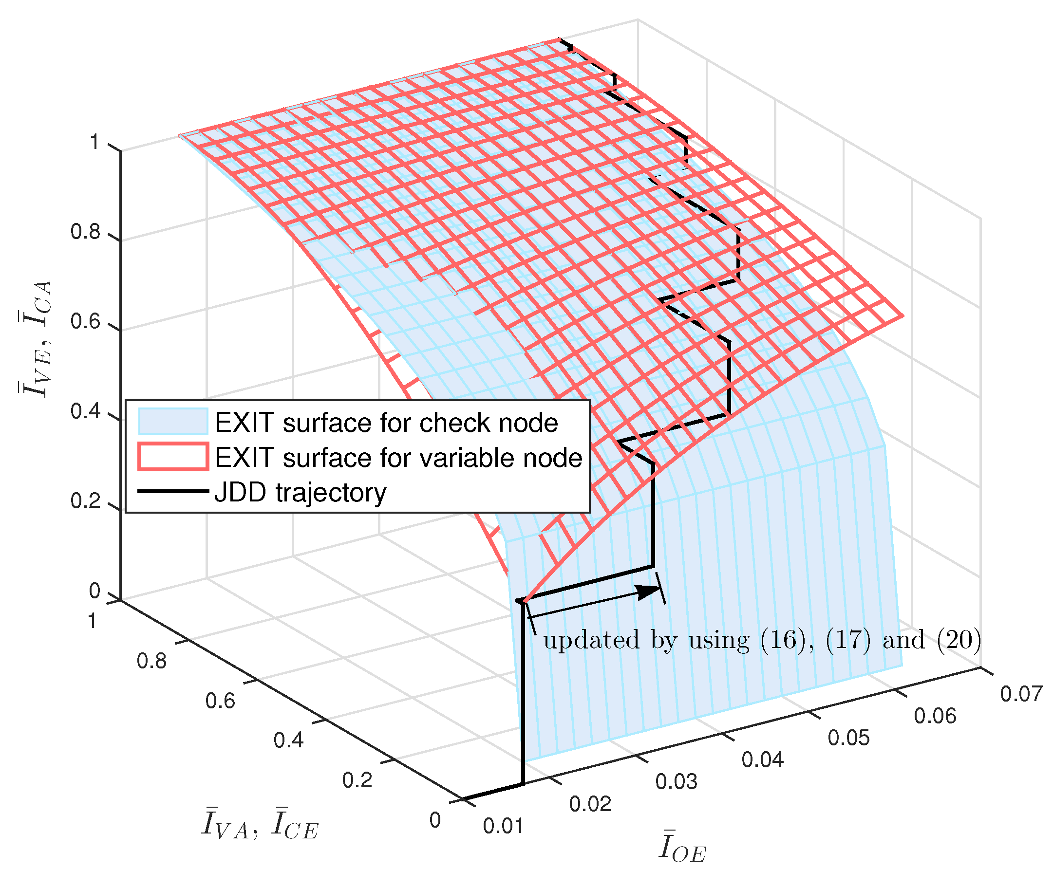
We can obtain the 3-D EXIT chart of JDD process by using Equations (
16)–(
22). The EXIT surface for variable nodes is obtained by using Equations (
18)–(
20). The EXIT surface for check nodes is obtained by stretching along the
-axis the 2-D EXIT function from
to
obtained by Equations (
21) and (
22). As an example, we plot in
Figure 4 the 3-D EXIT chart of JDD process for (3, 6)-regular LDPC coded massive MIMO systems with
and
, where coded bits are 4-QAM modulated and transmitted over
MIMO channel. We also plot in
Figure 4 the JDD trajectory obtained by Algorithm 3, where the update for
is computed by Equations (
16), (
17) and (
20). It is observed that the JDD trajectory is formed between two EXIT surfaces. If the JDD trajectory approaches a point with
at a certain
, this implies that the JDD converges and the decoding succeeds at this
. The minimum value of
resulting in the JDD trajectory approaching
is called the threshold. We can find the threshold value of LDPC coded massive MIMO system by using Algorithm 3 and visualize the JDD behavior by using the 3-D EXIT chart.
| Algorithm 3: Density evolution in terms of EXIT characteristics. |
![Entropy 21 00231 i003]() |


