Abstract
In this paper, a new lattice Boltzmann model for the two-component system of coupled sine-Gordon equations is presented by using the coupled mesoscopic Boltzmann equations. Via the Chapman-Enskog multiscale expansion, the macroscopical governing evolution system can be recovered correctly by selecting suitable discrete equilibrium distribution functions and the amending functions. The mesoscopic model has been validated by several related issues where analytic solutions are available. The experimental results show that the numerical results are consistent with the analytic solutions. From the mesoscopic point of view, the present approach provides a new way for studying the complex nonlinear partial differential equations arising in natural nonlinear phenomena of engineering and science.
1. Introduction
It is well known that most of the nonlinear phenomena that arise in engineering fields and mathematical physics, including plasma physics, fluid dynamics and nonlinear fiber optics, can be described by nonlinear partial differential equations (NPDEs). NPDEs have become an available tool for describing these natural nonlinear phenomena of engineering and science models. Hence, it becomes more and more important to be acquainted with all traditional and recently developed methods for NPDEs, and implementation of these methods [1,2]. Some of the most interesting features or physical rules are concealed in their nonlinear characteristics and can only be researched with an approximate method that is designed for inherent nonlinearity issues. As a result of the complexity and nonlinearity of the wave evolution equations, there is no uniform approach to obtain all solutions of the nonlinear wave evolution system. Hence, to find more precise and more effective methods for acquiring the nonlinear wave evolution equations has been an attractive research business. In the last few decades, quite a number of research work has been designed to research various types of nonlinear wave evolution equations. They include effective and broadly applicable techniques such as the finite difference method, variational iteration method, finite element method, finite volume method, boundary elements method, etc.
In recent years, lattice Boltzmann (LB) method has been developed as an optional numerical method to study nonlinear wave propagate equations and evolution of complexity physical system [3,4], especially in liquid mechanics [5,6,7,8]. Unlike more conventional numerical approaches, which are based on the discretization of macroscopic evolution equations, the LB method is based on the mesoscopic kinetic Boltzmann equations for discrete distribution functions. The basic viewpoint is to substitute the macroscopic hydrodynamic equations by a simplified mesoscopic equation modeled on the kinetic theory of gases. To get the hydrodynamic quantities, such as velocity, temperature, pressure, we use the Chapman-Enskog (C-E) multiscale expansion [9] which exploits a small parameter approximation to depict slowly varying solutions of the underlying kinetic evolution equations. This mesoscopic kinetic method has wide prospects in different areas, such as particle suspensions [10], approximate incompressible flows [11,12,13,14], compressible flows [15,16,17,18,19,20,21,22,23,24,25,26,27,28], biofilter media [29], and thermal multiphase flows [30]. Recently, the LB method has been successfully extended to some simulations of NPDEs, including the Korteweg-de Vries equation [31], the Gross-Pitaevskii equation [32], the convection-diffusion equation [33,34,35,36,37,38,39], the Poisson equation [40,41], the Kuramoto-Sivashinsky equation [42], the wave equation [43,44,45,46], the Dirac equation [47], etc. From the point view of calculation, its remarkable advantages include inherent parallelism, geometrical flexibility, numerical efficiency, simplicity of programming and simplicity in dealing with complex boundary conditions.
In this work, we consider the two-component system of coupled sine-Gordon equations, which was introduced recently by Khusnutdinova and Pelinovsky [48]. The basic one-dimensional form is shown as follows:
where remarks the ratio of the acoustic velocities between the components u and w, the dimensionless parameter is the same with the ratio of masses of particles in the “lower” and the “upper” parts of the crystal. This system produces the Frenkel-Kontorova dislocation model [49], and this system has also turned out to be highly suitable to describe fluxon phenomena of stacked intrinsic Josephson junctions in high temperature superconductors. Moreover, this system has been studied extensively for two-junction stacks, for stacks consisting of more junctions only some special cases have been analyzed [50]. In addition, this system (1) with was proposed to describe the open states in DNA [51].
We consider the above system (1) with the initial conditions as follows:
and the boundary conditions:
where , , , and are known functions.
There are many analytical methods solving the two-component system of coupled sine-Gordon equations, such as the modified decomposition method [52], the homotopy analysis method [53], the hyperbolic auxiliary function method [54], the homotopy perturbation method [55], the rational exponential ansatz method [56], the variational iteration method [57] and the modified Kudryashov method [58]. However, to our best knowledge, there are few numerical method to solve this coupled system. In recent years, the studies in Refs. [33,59,60] show that the LB method may be an valid numerical solver for real and complex nonlinear coupled systems. Therefore, it is worthy to more study LB method and enlarge its applications. As far as we know, there is no LB model for the two-component system of coupled sine-Gordon equations. The system has similar structure of the convection-diffusion system except for the second time derivative. We can define the first derivatives of macroscopic variable as the sum of distribution functions by the thought of the reference [44]. The main goal of this work is to extend the LB model to solve this two-component system of coupled sine-Gordon numerically by using the double mesoscopic Boltzmann equations. Through the C-E multiscale expansion, the governing nonlinear coupled evolution equations are recovered accurately from the double continuous Boltzmann equations. In order to compare the numerical solutions with the analytic ones, three test problems are taken into account. It is found that the numerical solutions are in accordance with the analytical ones. This demonstrates that the present model is an valid and flexible way for actual application.
The content of this paper is arranged as follows. Next section shows our LB model for the coupled sine-Gordon equations for the two-component system through the present model. Numerical validation is presented in Section 3. Finally, a brief summary is made.
2. Lattice Boltzmann Model
In the present model, the three-velocity lattice Bhatnagar-Gross-Krook (BGK) model is used. The directions of the particle discrete velocity are defined as :
The LB equation with double distribution functions for and are given as follows :
where and refer to the distribution function and equilibrium distribution function, respectively. is defined as an amending function, c is a constant to determine the viscous coefficient, is the time step, the dimensionless single-relaxation-time which regulates the rate of approach to the equilibrium. The stability of the equation needs [61].
Unlike the normal LB method, the first derivatives of macroscopic variables and are defined [44] as follows:
Thus, the steady macroscopical quantities meet the following conservative conditions:
Afterwards, through choosing appropriate local equilibrium distributions and amending functions, the corresponding macroscopic coupled system can be retrieved correctly.
Next, we will give the detailed derivation. Applying the Taylor expansion to the left-hand side of Equation (5) about the point x and t, we can obtain :
By introducing the C-E multiscale expansions, we can expand the distribution function around as follows:
And are the non-equilibrium distribution functions, which satisfy the solvability conditions :
Comparing the two sides of Equation (11) and setting terms of order to each other, we have :
Therefore:
Comparing the two sides of Equation (11) and setting terms of order to each other, we get :
According to the macroscopic equations, the local equilibrium distribution function is required to satisfy the following relations:
in terms of:
Meanwhile, the source term satisfies:
Meanwhile, from Equation (19), we can get the local equilibrium distribution functions as:
From Equation (21), the amending functions can be determined. For the sake of simplicity, only one case is presented here:
and:
In the simulation process, in order to get and , we can apply the backward difference to the items and as:
and:
then using Equation (6), we get:
and:
3. Numerical Simulation
In order to test the accuracy and efficiency of the present LB model, three initial and boundary value problems which have analytical solutions are simulated.
For the sake of numerical stability of the finite LB scheme, is adopt in all simulations. Initially, the distribution functions are set to equal . And the macroscopic variables and in Equation (1) are set to equal the initial conditions. The initial and boundary conditions of the test problems with analytical solutions are content with their analytical solutions. The non-equilibrium extrapolation scheme [62] is adopted to deal with the boundary condition.
Firstly, let us introduce symbols , , , , , n is the nth layer time, j is the spatial grid. Then we can reformulate the LB Equation (5) by the classical finite difference notation:
At time , u and w are updated as follows:
and:
The initial local equilibrium distribution functions are:
where , , and .
The global relative error (GRE) is introduced to measure the present model’s precision, and defined as follows:
where , represent the numerical solution and analytical one, respectively. The summation is taken all grid points together. Next, numerical tests are performed for different initial conditions of the coupled sine-Gordon equations. It is found that the numerical solutions are in accordance with the analytical solutions over a relatively long period of time.
Example 1.
Consider the two-component system of coupled sine-Gordon equations in the region given as:
with the initial conditions:
and the analytical solution for this problem is extracted from Ref. [56] by:
where . The boundary conditions conform to the analytical solution.
In the proceeding, we adopt , , , , . The computational region is fixed on . The global relative errors (GRE) for the solutions and at with different resolutions, from to 80, and the space grid N from 400 to 3200, are listed in Table 1 and Table 2. From these two tables, we can see that GREs for are found to range from to , and GREs for are found to range from to . We can also see that when is larger, namely is relatively smaller, the global relative error of reduces with the first-order accuracy, while the global relative error of changes little. The accuracy of the macroscopic variable is not affected by the resolution in space and time. That is due to the treatment of the items and in Equations (31) and (32), has the first-order accuracy. According to Table 1 and Table 2, we adopt in consideration of both the computational accuracy and efficiency. It can be found that the numerical results in according with the analytical solutions, which are presented as the spatiotemporal evolution graph of the numerical (left) and analytical (right) solutions for comparison, see Figure 1 and Figure 2. For clarity of contrast, we also present the two-dimensional visual comparisons of (left) and (right) at , see Figure 3. It is evident that the numerical results coincide with the analytical solutions.
Example 2.
Consider the two-component system of coupled sine-Gordon equations in the region given by:
with the discontinuous initial conditions:
and the analytical solution for this problem is extracted from Reference [56] by:
where . The boundary conditions conform to the analytical solution.

Table 1.
The global relative error (GRE) for with different .
Table 2.
The global relative error (GRE) for with different .
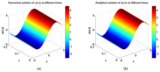
Figure 1.
Spatiotemporal evolution graph of the numerical (a) and analytical (b) solutions up to s, with for Example 1.
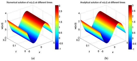
Figure 2.
Spatiotemporal evolution graph of the numerical (a) and analytical (b) solutions up to s, with for Example 1.
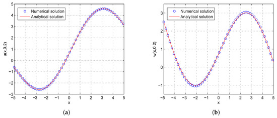
Figure 3.
Comparison between numerical and analytical solutions of (a) and (b) at with for Example 1. The blue circle symbol represents the numerical solution, and the solid red line represents the analytical solution given by Equation (42).
In the proceeding, we adopt , , , , . The computational region is fixed within . The GREs for the solutions and at in different resolutions, from to 80 and the space grid N from 400 to 3200, are listed in Table 3 and Table 4. From these two tables, we can see that the GREs for range from to , and the GREs for range from to . When is larger, namely is relatively small, the GREs of reduces with first-order accuracy, the GREs of change little. At the same time, we present the spatiotemporal evolution graph of the numerical (left) and analytical (right) solutions of and for comparison, see Figure 4 and Figure 5. For clarity of contrast, we also present the two-dimensional visual comparisons of (left) and (right) at , see Figure 6. It can be found that the numerical results in according with the analytical solutions.
Example 3.
Consider the two-component system of coupled sine-Gordon equations in the region given by:
with the initial conditions:
and the analytical solution for this problem is extracted from Reference [56] by:
where . The boundary conditions conform to the analytical solution.
Table 3.
The global relative error (GRE) for with different .
Table 4.
The global relative error (GRE) for with different .
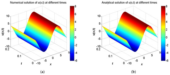
Figure 4.
Spatiotemporal evolution graph of the numerical (a) and analytical (b) solutions up to t = 0.2 s, with for Example 2.
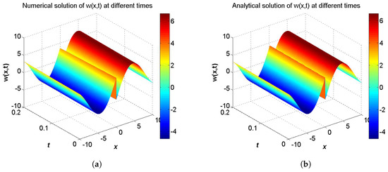
Figure 5.
Spatiotemporal evolution graph of the numerical (a) and analytical (b) solutions up to t = 0.2 s, with for Example 2.
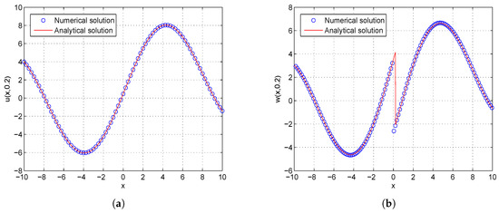
Figure 6.
Comparison between numerical and analytical solutions of (a) and (b) at with for Example 2. The blue circle symbol represents the numerical solution, and the solid red line represents the analytical solution given by Equation (45).
In the proceeding, we adopt , , , , . The computational region is fixed within . The GREs for the solutions and at in different resolutions, from to 80 and the space grid N from 400 to 3200, which are listed in Table 5 and Table 6. From these two tables, we can see that the GREs for are found to range from to , and the GREs for are found to range from to . When is larger, namely is relatively small, the global relative error of reduces with first-order accuracy, the GREs of changes little. At the same time, we present the spatiotemporal evolution graph of the numerical (left) and analytical (right) solutions for comparison, see Figure 7 and Figure 8. For clarity of contrast, we also present the two-dimensional visual comparisons of (left) and (right) at , see Figure 9. It can be found that the numerical results in according with the analytical solutions.
Table 5.
The global relative error (GRE) for with different .
Table 6.
The global relative error (GRE) for with different .
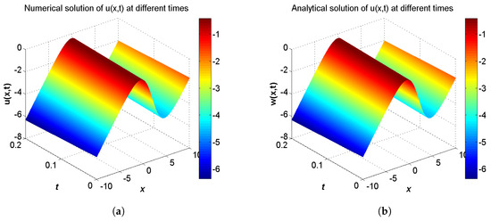
Figure 7.
Spatiotemporal evolution graph of the numerical (a) and analytical (b) solutions up to s, with for Example 3.
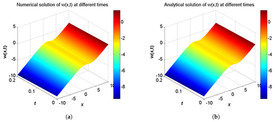
Figure 8.
Spatiotemporal evolution graph of the numerical (a) and analytical (b) solutions up to s, with for Example 3.
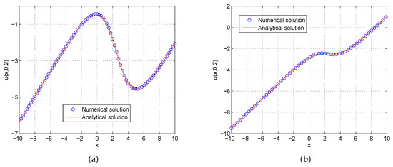
Figure 9.
Comparison between numerical and analytical solutions of (a) and (b) at with for Example 3. The blue circle symbol represents the numerical solution, and the solid red line represents the analytical solution given by Equation (48).
4. Conclusions
In conclusion, we have researched the application of the LB method for the solution of the two-component system of coupled sine-Gordon equations. By choosing the equilibrium distribution function and an amending function suitably, according to our proposed model, the governing evolution equations can be recovered accurately, in which the Chapman-Enskog multiscale expansion is employed. Numerical simulation for three test problems has been conducted to validate the LB model. The numerical results are in good agreement with the analytical solutions. While we take different initial conditions, we can get unique numerical solutions. We can also see that when is larger, is relatively smaller, and the global relative error of reduces with first-order accuracy; nevertheless, the global relative error of changes little. It is found that the accuracy of the macroscopic variable is not affected by the resolution in space and time. That is due to the treatment of the items and in Equations (31) and (32), which have first-order accuracy. For the purpose of attaining better computational accuracy and efficiency, the LB method for the test problems needs relatively small time step and space step. The present model can be developed to research more different types of the nonlinear system problems. There are still many problems worth studying to develop the present method, such as how to improve the accuracy and stability; we will continue these study in the near feature.
Author Contributions
Conceptualization, D.L. and H.L.; Methodology, D.L. and H.L.; Investigation, D.L. and C.L.; Validation, H.L. and C.L.; Visualization, D.L. and H.L.; Writing—original draft preparation, D.L.; Writing—review and editing, H.L. and C.L.; Supervision, H.L.; Project administration, H.L.; Funding acquisition, H.L.
Funding
This work was supported by National Natural Science Foundation of China (under Grant Nos. 11301082,51806116) and Natural Science Foundation of Fujian Provinces (under Grant Nos. JT180075, 2018J01654).
Conflicts of Interest
The authors declare no conflict of interest.
References
- Baskonus, H.; Bulut, H. New hyperbolic function solutions for some nonlinear partial differential equation arising in mathematical physics. Entropy 2015, 17, 4255–4270. [Google Scholar] [CrossRef]
- Vitanov, N.K.; Dimitrova, Z.I.; Vitanov, K.N. Modified method of simplest equation for obtaining exact analytical solutions of nonlinear partial differential equations: further development of the methodology with applications. Appl. Math. Comput. 2015, 269, 363–378. [Google Scholar] [CrossRef]
- Benzi, R.; Succi, S.; Vergasola, M. The lattice Boltzmann equation: Theory and applications. Phys. Rep. 1992, 222, 145–197. [Google Scholar] [CrossRef]
- Succi, S. Lattice boltzmann 2038. Europhys. Lett. 2015, 109, 50001. [Google Scholar] [CrossRef]
- Chen, S.Y.; Doolen, G.D. Lattice Boltzmann method for fluid flows. Annu. Rev. Fluid Mech. 1998, 30, 329–364. [Google Scholar] [CrossRef]
- Aidun, C.K.; Clausen, J.R. Lattice-Boltzmann method for complex flows. Annu. Rev. Fluid Mech. 2010, 42, 439–472. [Google Scholar] [CrossRef]
- Xu, A.G.; Zhang, G.C.; Gan, Y.B.; Chen, F.; Yu, X.J. Lattice Boltzmann modeling and simulation of compressible flows. Front. Phys. 2012, 7, 582–600. [Google Scholar] [CrossRef]
- Li, Q.; Luo, K.H.; Kang, Q.J.; He, Y.L.; Chen, Q.; Liu, Q. Lattice Boltzmann methods for multiphase flow and phase-change heat transfer. Prog. Energy Combust. Sci. 2016, 52, 62–105. [Google Scholar] [CrossRef]
- Chapman, S.; Cowling, T.G. The Mathematical Theory of Non-Uniform Gases, 3rd ed.; Cambridge University: London, UK, 1970. [Google Scholar]
- Stratford, K.; Pagonabarraga, I. Parallel simulation of particle suspensions with the lattice Boltzmann method. Comput. Math. Appl. 2008, 55, 1585–1593. [Google Scholar] [CrossRef]
- Li, Q.; Luo, K.H. Effect of the forcing term in the pseudopotential lattice Boltzmann modeling of thermal flows. Phys. Rev. E 2014, 89, 053022. [Google Scholar] [CrossRef]
- Liu, H.H.; Wu, L.; Ba, Y.; Xi, G.; Zhang, Y.H. A lattice Boltzmann method for axisymmetric multicomponent flows with high viscosity ratio. J. Comput. Appl. 2016, 327, 873–893. [Google Scholar] [CrossRef]
- Wang, Y.; Shu, C.; Huang, H.B.; Teo, C.J. Multiphase lattice Boltzmann flux solver for incompressible multiphase flows with large density ratio. J. Comput. Appl. 2015, 280, 404–423. [Google Scholar] [CrossRef]
- Wei, Y.K.; Wang, Z.D.; Qian, Y.H.; Guo, W.J. Study on bifurcation and dual solutions in natural convection in a horizontal annulus with rotating inner cylinder using thermal immersed boundary-lattice Boltzmann method. Entropy 2018, 20, 733. [Google Scholar] [CrossRef]
- Gan, Y.B.; Xu, A.G.; Zhang, G.C.; Succi, S. Discrete Boltzmann modeling of multiphase flows: Hydrodynamic and thermodynamic non-equilibrium effects. Soft Matter 2015, 11, 5336–5345. [Google Scholar] [CrossRef] [PubMed]
- Zhang, Y.D.; Xu, A.G.; Zhang, G.C.; Zhu, C.M.; Lin, C.D. Kinetic modeling of detonation and effects of negative temperature coefficient. Combust. Flame 2016, 173, 483–492. [Google Scholar] [CrossRef]
- Gan, Y.B.; Xu, A.G.; Zhang, G.C.; Zhang, Y.D.; Succi, S. Discrete Boltzmann trans-scale modeling of high-speed compressible flows. Phys. Rev. E 2018, 97, 053312. [Google Scholar] [CrossRef] [PubMed]
- Zhang, Y.D.; Xu, A.G.; Zhang, G.C.; Chen, Z.H.; Wang, P. Discrete ellipsoidal statistical BGK model and Burnett equations. Front. Phys. 2018, 13, 135101. [Google Scholar] [CrossRef]
- Chen, F.; Xu, A.G.; Zhang, G.C. Collaboration and competition between Richtmyer-Meshkov instability and Rayleigh-Taylor instability. Front. Phys. 2018, 30, 102105. [Google Scholar]
- Xu, A.G.; Zhang, G.C.; Zhang, Y.D.; Wang, P.; Ying, Y.J. Discrete Boltzmann model for implosion- and explosion-related compressible flow with spherical symmetry. Front. Phys. 2018, 13, 135102. [Google Scholar] [CrossRef]
- Gan, Y.B.; Xu, A.G.; Zhang, G.C.; Lin, C.D.; Lai, H.L.; Liu, Z.P. Nonequilibrium and morphological characterizations of Kelvin-Helmholtz instability in compressible flows. Front. Phys. 2019, 14, 43602. [Google Scholar] [CrossRef]
- Lin, C.D.; Xu, A.G.; Zhang, G.C.; Li, Y.J. Double-distribution-function discrete Boltzmann model for combustion. Combust Flame 2016, 164, 137–151. [Google Scholar] [CrossRef]
- Lin, C.D.; Luo, K.H.; Fei, L.L.; Succi, S. A multi-component discrete Boltzmann model for nonequilibrium reactive flows. Sci. Rep. 2017, 7, 14580. [Google Scholar] [CrossRef] [PubMed]
- Lin, C.D.; Luo, K.H. MRT discrete Boltzmann method for compressible exothermic reactive flows. Combust Flame 2018, 166, 176–183. [Google Scholar] [CrossRef]
- Lai, H.L.; Xu, A.G.; Zhang, G.C.; Gan, Y.B.; Ying, Y.J.; Succi, S. Nonequilibrium thermohydrodynamic effects on the Rayleigh-Taylor instability in compressible flows. Phys. Rev. E 2016, 94, 023106. [Google Scholar] [CrossRef] [PubMed]
- Zhang, Y.D.; Xu, A.G.; Zhang, G.C.; Gan, Y.B.; Chen, Z.H.; Succi, S. Entropy production in thermal phase separation: A kinetic-theory approach. Soft Matter 2019, 15, 2245–2259. [Google Scholar] [CrossRef] [PubMed]
- Xu, A.G.; Zhang, G.C.; Ying, Y.J.; Wang, C. Complex fields in heterogeneous materials under shock: Modeling, simulation and analysis. Sci. China-Phys. Mech. Astron. 2016, 59, 650501. [Google Scholar] [CrossRef]
- Zhang, Y.D.; Xu, A.G.; Zhang, G.C.; Chen, Z.H.; Wang, P. Discrete Boltzmann method for non-equilibrium flows: Based on Shakhov model. Comput. Phys. Commun. 2019, 238, 50–65. [Google Scholar] [CrossRef]
- Yan, W.W.; Su, Z.D.; Zhang, H.J. Effect of non-isothermal condition on heterogeneous flow through biofilter media by lattice Boltzmann simulation. J. Chem. Technol. Biotechnol. 2013, 88, 456–461. [Google Scholar] [CrossRef]
- Li, Q.; Kang, Q.J.; Francois, M.M.; He, Y.L.; Luo, K.H. Lattice Boltzmann modeling of boiling heat transfer: The boiling curve and the effects of wettability. Int. J. Heat Mass Tran. 2015, 85, 787–796. [Google Scholar] [CrossRef]
- Wang, H.M. Solitary wave of the Korteweg-de Vries equation based on lattice Boltzmann model with three conservation laws. Adv. Space Res. 2017, 59, 283–292. [Google Scholar] [CrossRef]
- Wang, H.M.; Yan, G.W. Lattice Boltzmann model for the interaction of (2+1)-dimensional solitons in generalized Gross-Pitaevskii equation. Appl. Math. Model. 2016, 40, 5139–5152. [Google Scholar] [CrossRef]
- Chai, Z.H.; He, N.Z.; Guo, Z.L.; Shi, B.C. Lattice Boltzmann model for high-order nonlinear partial differential equations. Phys. Rev. E 2018, 97, 013304. [Google Scholar] [CrossRef] [PubMed]
- Shi, B.C.; Guo, Z.L. Lattice Boltzmann model for nonlinear convection-diffusion equations. Phys. Rev. E 2009, 79, 016701. [Google Scholar] [CrossRef] [PubMed]
- Yoshida, H.; Nagaoka, M. Lattice Boltzmann method for the convection-diffusion equation in curvilinear coordinate systems. J. Comput. Phys. 2014, 257, 884–900. [Google Scholar] [CrossRef]
- Chai, Z.H.; Zhao, T.S. Lattice Boltzmann model for the convection-diffusion equation. Phys. Rev. E 2013, 87, 063309. [Google Scholar] [CrossRef] [PubMed]
- Chai, Z.H.; Shi, B.C.; Guo, Z.L. A multiple-relaxation-time lattice Boltzmann model for general nonlinear anisotropic convection-diffusion equations. J. Sci. Comput. 2016, 69, 355–390. [Google Scholar] [CrossRef]
- Wang, L.; Chai, Z.H.; Shi, B.C. Regularized lattice Boltzmann simulation of double-diffusive convection of power-law nanofluids in rectangular enclosures. Int. J. Heat Mass Transfer 2016, 102, 381–395. [Google Scholar] [CrossRef]
- Wang, L.; Shi, B.C.; Chai, Z.H. Regularized lattice Boltzmann model for a class of convection-diffusion equations. Phys. Rev. E 2015, 92, 043311. [Google Scholar] [CrossRef]
- Chai, Z.H.; Shi, B.C. A novel lattice Boltzmann model for the Poisson equation. Appl. Math. Model 2008, 32, 2050–2058. [Google Scholar] [CrossRef]
- Wang, H.M.; Yan, W.W.; Yan, B. Lattice Boltzmann model based on the rebuilding-divergency method for the Laplace equation and the Poisson equation. J. Sci. Comput. 2011, 46, 470–484. [Google Scholar] [CrossRef]
- Lai, H.L.; Ma, C.F. Lattice Boltzmann method for the generalized Kuramoto-Sivashinsky equation. Physica A 2009, 388, 1405–1412. [Google Scholar] [CrossRef]
- Lai, H.L.; Ma, C.F. Lattice Boltzmann model for generalized nonlinear wave equations. Phys. Rev. E 2011, 84, 046708. [Google Scholar] [CrossRef] [PubMed]
- Yan, G.W. A lattice Boltzmann equation for waves. J. Comput. Phys. 2000, 161, 61–69. [Google Scholar]
- Lai, H.L.; Ma, C.F. Numerical study of the nonlinear combined Sine-Cosine-Gordon equation with the lattice Boltzmann method. J. Sci. Comput. 2012, 53, 569–585. [Google Scholar] [CrossRef]
- Duan, Y.L.; Kong, L.H.; Guo, M. Numerical simulation of a class of nonlinear wave equations by lattice Boltzmann method. Commun. Math. Stat. 2017, 5, 13–35. [Google Scholar] [CrossRef]
- Shi, B.C.; Guo, Z.L. Lattice Boltzmann model for the one-dimensional nonlinear Dirac equation. Phys. Rev. E 2009, 79, 066704. [Google Scholar] [CrossRef] [PubMed]
- Khusnutdinova, K.R.; Pelinovsky, D.E. On the exchange of energy in coupled Klein-Gordon equations. Wave Motion 2003, 38, 1–10. [Google Scholar] [CrossRef]
- Braun, O.M.; Kivshar, Y.S. Nonlinear dynamics of the Frenkel-Kontorova model. Phys. Rep. 1998, 306, 1–108. [Google Scholar] [CrossRef]
- Kleiner, R.; Gaber, T.; Hechtfischer, G. Josephson Stacked long junctions in external magnetic fields-a numerical study of coupled one-dimensional sine-Gordon equations. Physica C 2001, 362, 29–37. [Google Scholar] [CrossRef]
- Yomosa, S. Soliton excitations in deoxyribonucleic acid (DNA) double helices. Phys. Rev. A 1983, 27, 2120–2125. [Google Scholar] [CrossRef]
- Saha, R.S. A numerical solution of the coupled sine-Gordon equation using the modified decomposifition method. Appl. Math. Comput. 2006, 175, 1046–1054. [Google Scholar]
- Bataineh, A.S.; Noorani, M.S.M.; Hashim, I. Approximate analytical solutions of systems of PDEs by homotopy analysis method. Comput. Math. Appl. 2008, 55, 2913–2923. [Google Scholar] [CrossRef]
- Zhao, Y.M.; Liu, H.H.; Yang, Y.J. Exact solutions for the coupled Sine-Gordon equations by a new hyperbolic auxiliary function method. Appl. Math. Sci. 2011, 5, 1621–1629. [Google Scholar]
- Darvishi, M.T.; Khani, F.; Hamedi-Nezhad, S.; Ryu, S.W. New modification of the HPM for numerical solutions of the sine-Gordon and coupled sine-Gordon equations. Int. J. Comput. Math. 2010, 87, 908–919. [Google Scholar] [CrossRef]
- Salas, A.H. Exact solutions for the coupled sine-Gordon equations. Nonlinear Anal: Real World Appl. 2010, 11, 3930–3935. [Google Scholar] [CrossRef]
- Batiha, B.; Noorani, M.S.M.; Hashim, I. Approximate analytical solution of the coupled sine-Gordon equation using the variational iteration method. Phys. Scr. 2007, 76, 445–448. [Google Scholar] [CrossRef]
- Hosseini, K.; Mayeli, P.; Kumar, D. New exact solutions of the coupled sine-Gordon equations in nonlinear optics using the modified Kudryashov method. J. Mod. Optic. 2018, 65, 361–364. [Google Scholar] [CrossRef]
- Shi, B.C. Lattice Boltzmann simulation of some nonlinear complex equations. Lect. Notes Comput. Sci. 2007, 4487, 818–825. [Google Scholar]
- Liu, F.; Shi, W.P. Numerical solutions of two-dimensional Burgers’ equations by lattice Boltzmann method. Commun. Nonlinear Sci. Numer. Simul. 2011, 16, 150–157. [Google Scholar] [CrossRef]
- Sterling, J.D.; Chen, S.Y. Stability analysis of lattice Boltzmann methods. J. Comput. Phys. 1996, 123, 196–206. [Google Scholar] [CrossRef]
- Guo, Z.L.; Zheng, C.G.; Shi, B.C. An extrapolation method for boundary conditions in lattice Boltzmann method. Phys. Fluids 2002, 14, 2007–2010. [Google Scholar] [CrossRef]


© 2019 by the authors. Licensee MDPI, Basel, Switzerland. This article is an open access article distributed under the terms and conditions of the Creative Commons Attribution (CC BY) license (http://creativecommons.org/licenses/by/4.0/).