Based on the analysis of how graphical symmetry affects isomorphism detection, we proposed the MapEff algorithm with its main implementation procedures in this section. To help understand how MapEff obtains the correct isomorphism mapping between regular graphs, a pair of graphs are used as the instance for the description. After completing this algorithm, further discussion about the computation complexity is also presented here.
3.1. The Impact of Symmetry in Isomorphism Detection
Regular graphs has strong symmetry, as each vertex has the same number of neighbors. This symmetry introduces many equivalent nodes, and even results in automorphism, which means the graph can map itself through a structure-preserving permutation mapping. Even though quantum walk, as a novel quantum computation model, is sensitive to the topological structure and can establish the unit bijection effectively based on the analysis of probability amplitude, too many candidate unit bijections in a symmetric graph will bring in complex combinations and make it difficult to integrate the correct isomorphic mapping. Therefore, a strong symmetric graph limits the application of these quantum-inspired isomorphism.
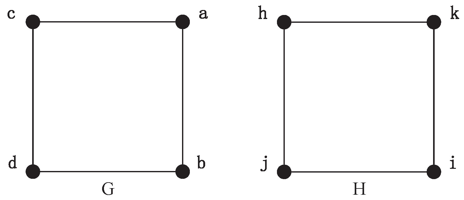
For example, two square graphs,
G and
H, are shown in
Figure 1. Each of them has four equivalent nodes and four edges. Obviously, these two graphs are isomorphic. When we perform the Emms-D algorithm to explore the isomorphic mapping of them, an auxiliary graph is constructed firstly by adding a layer of auxiliary vertices and some extra edges to connect two graphs, as shown in
Figure 2. This auxiliary graph has 24 vertices and 40 edges. Each node in the
G graph is connected to every vertice in
H by an auxiliary node. We describe the auxiliary node to connect vertex
a and
h as
, and the rest of the auxiliary nodes are expressed similarly. Then the DTQW is simulated on the auxiliary graph. The auxiliary edges with the same probability amplitude reveal the unit bijections in isomorphic mapping. If the auxiliary edges connected to the same auxiliary node have the same probability amplitude, a unit bijection between the corresponding vertices is established. Because both
G and
H have four equivalent nodes, we can see that all probability amplitude of auxiliary edges are always the same, as shown in
Table 1. That is to say each node in
G can establish a unit bijection with any node in graph
H. In order to integrate the unit bijections into isomorphic mapping, we need to choose four unit bijections from 16 candidates. It is not easy to guarantee the combination of these unit bijections can generate the right isomorphic mapping, even under the constrain that each node can only be used once. For instance, the output can be
. Obviously, this result is not structure-preserving because vertex
b and
d are adjacent, but
j and
k are not. Therefore, the key issue is to figure out the right one from the candidate unit bijections. Unfortunately, few previous studies have focused on this problem, since most of them just establish unit bijection one by one and simply integrate unit bijections into the isomorphism mapping function. By the random selection of candidate unit bijections, the probability to get the right isomorphic mapping seems unsatisfactory, especially when the graph have too many equivalent vertices. Therefore, an efficient algorithm to map with regular graph isomorphism is necessary.
Unfortunately, most algorithms only make little effort to deal with this problem. They establish unit bijection one by one and simply integrate unit bijections into the isomorphism mapping function. Hence, it is difficult for them to discover the isomorphism mapping between regular graphs. Although the correct graph isomorphic mapping sometimes can be obtained by random selection, the possibility is also very small, especially when the graph have too many equivalent vertices. Therefore, an efficient algorithm for coping with regular graph isomorphism is needed.
3.2. Detailed Mechanism of MapEff
In this subsection, we introduce the detailed procedures of MapEff algorithm on two graphs and . The process of this algorithm can be roughly divided into the following steps. First, all candidate matching nodes for each vertex are selected based on the NodeMap testing. This strategy is inspired by Emms-D algorithm. It first builds the auxiliary graph through connecting the two testing nodes. Then we utilize the amplitudes computed in DTQW simulation to validate the matching. If there is only one candidate, , the unit bijection is added to the isomorphic mapping function. For the case of multiple candidates, MapEff needs to identify the most suitable one based on the existing unit bijections. In the most extreme case, if none of the candidates is available, we can conclude that G and H are not isomorphic. After the unit bijections are established one by one, we can acquire the correct isomorphic mapping function.
To ensure that the DTQW can be simulated, we add a self-loop to each isolated vertex from G and H which can avoid the case that the degree of vertex is 0. Obviously, this pretreatment does not affect mapping function when two graphs are isomorphic.
Step 1: Select candidate matching nodes for each vertex in
G. To judge whether the node
is one of candidate mapping nodes of
, an auxiliary graph
defined in Equation (8) is constructed through adding an extra node
to connect vertex
and
.
Then the DTQW is executed on this auxiliary graph. If the quantum amplitudes of basic state representing edge and are equal, is considered as one of candidate mapping nodes of . This method is inspired by the Emms-D algorithm, which conducts DTQW on a big auxiliary graph that connects all pairs of vertices from two graphs. The difference is that we simplify the construction of auxiliary graph. The details of node matching algorithm are indicated in Algorithm 1.
| Algorithm 1 NodeMap |
| Input: |
| Output: |
- 1:
Construct auxiliary graph through adding an extra node c connecting u and v - 2:
Get the amplitude of basic states representing edge and based on the DTQW and store them in and , respectively. - 3:
ifthen - 4:
- 5:
else - 6:
- 7:
end if
|
Step 2: Preliminary match. If there is only one candidate matching node for , is considered as a unit bijection and added to isomorphic mapping function. When each vertex has multiple candidate matching nodes, we need to accept the first pair of candidate matching nodes as a unit bijection and put it in isomorphic mapping in order to continue.
Step 3: Determine the isomorphic mapping. After Step 2, at least one unit bijection in the isomorphic mapping function has been obtained. Next, we need to filter the remaining pairs of matching nodes through multiple iterations. When there are multiple candidate matching nodes for a vertex, we can rely on the existing determined unit bijection to choose the suitable one.
For instance, if we know that
is a unit bijection and
is one of the candidate matching node for
, graph
and
defined in Equations (9)–(10) are constructed through adding an edge to connect
and
,
and
, respectively. Of course, if
appears in the previously verified unit bijections, it is not a real candidate matching node and should be ignored.
Then the node matching algorithm (NodeMap) is performed to determine whether and are a pair of matching nodes. If , is considered as one suitable candidate and the unit bijection is accepted in isomorphic mapping function. Otherwise, this candidate unit bijection is rejected. Through adding auxiliary edges, the symmetry in the original graph can be reduced and MapEff can distinguish the equivalent vertices in a graph. Because the unit bijection is accepted and both graphs and use the same constructing method, the matching result of vertices and is not changed in these updated graphs. That is to say the isomorphic mapping between updated graphs and can be effective in graph G and H when they are isomorphic.
In this way, Algorithm 2 can further screen other candidate matching nodes based on this updated graphs. When unit bijection is accepted, the auxiliary graphs and constructed during this iteration is remained for the next round. This means every time a unit bijection is accepted, one edge is added to change the topological structure of the graph, thus reducing the symmetry in the regular graph. After several iterations, we can finally get the right isomorphic mapping function of two isomorphic graphs.
| Algorithm 2 MapEff |
| Input: |
| Output: isomorphism mapping function |
- 1:
Add a loop to each isolated point in the graph G and H - 2:
for each vertex do - 3:
for each vertex do - 4:
if then - 5:
- 6:
end if - 7:
end for - 8:
end for - 9:
for each vertex do - 10:
if then - 11:
- 12:
end if - 13:
if then - 14:
(The two graphs are not isomorphism.) - 15:
end if - 16:
end for - 17:
ifthen - 18:
The first appeared candidate unit bijection is added to isomorphism mapping. - 19:
end if - 20:
for each vertex do - 21:
for each do - 22:
Construct the auxiliary graph and - 23:
if then - 24:
- 25:
Store the auxiliary graph and for next iteration. - 26:
break - 27:
end if - 28:
end for - 29:
end for
|
3.3. Case Study
This section introduces an example of graph isomorphism detection based on the MapEff algorithm. We perform this algorithm on a pair of square graphs, as shown in
Figure 1. Square graph is a kind of regular graph with high symmetry, and we can indicate how the MapEff works out a correct isomorphic mapping by selecting suitable unit bijections on these graph.
At first, MapEff chooses all the candidate unit bijections based on the DTQW. In each selection, the MapEff constructs an auxiliary graph by connecting two graphs. We assume that it chooses vertex
a and
h to determine whether they can form a candidate unit bijection. The graph in
Figure 3 is the auxiliary graph in this procedure. Since the auxiliary edges of
and
have the same amplitude after simulating DTQW, we can establish a candidate unit bijection
. Through comparing every node pair by this way, all the candidate unit bijections from two graphs are obtained as shown in
Table 2. Under the constrain that each vertex is utilized only once, we need to choose four unit bijections and combine them into an isomorphic mapping.
After executing the above procedures, each vertex has four candidate matching nodes. In order to perform the next steps, MapEff selects the first candidate unit bijection
and adds it into the isomorphic mapping. Based on this accepted unit bijection, MapEff decides the matching node of vertex
b. As the node
h has appeared in the previously determined unit bijection (
), it will no longer be a matching node for
b, and the candidate unit bijection (
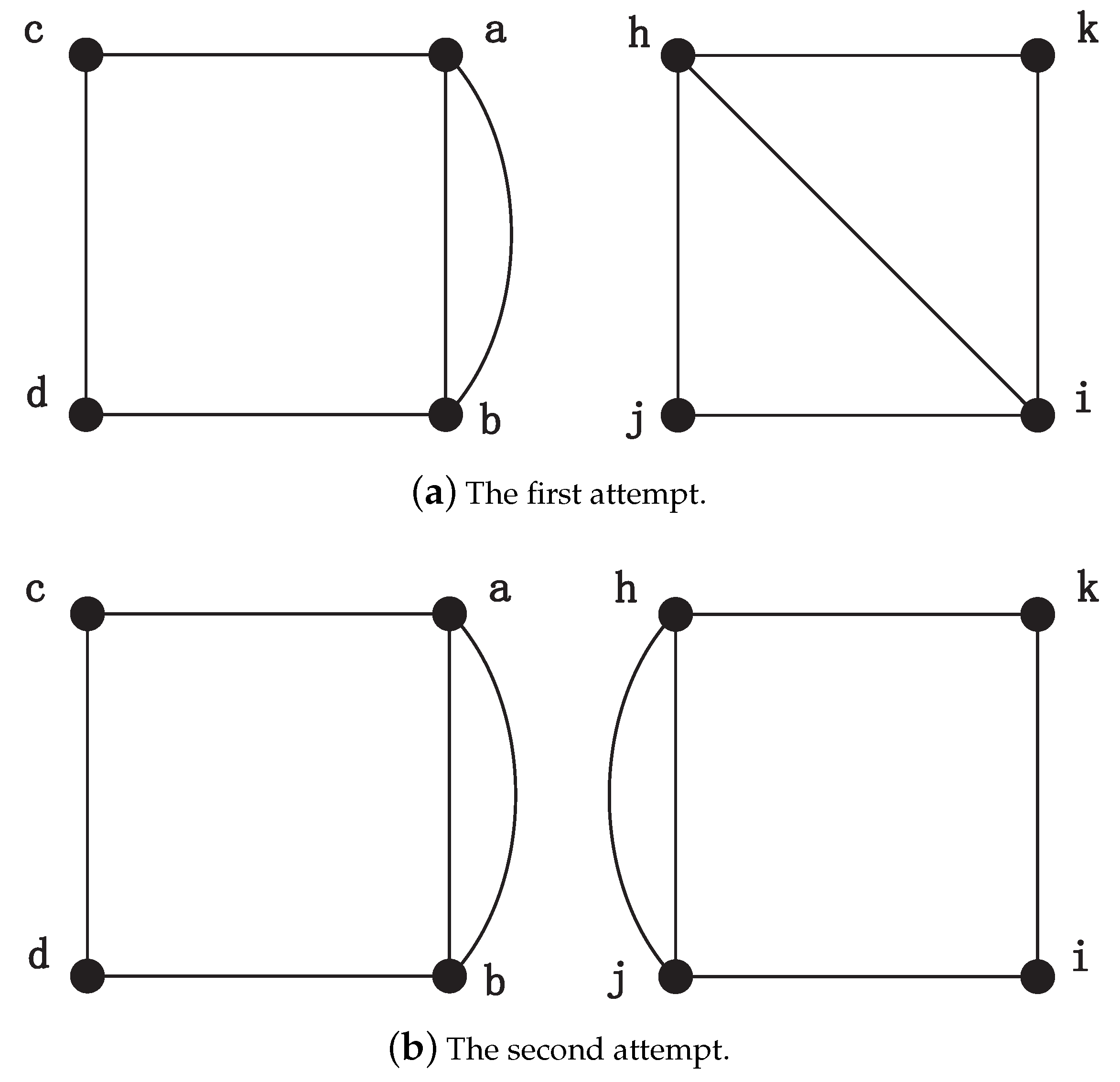
) will be disregarded directly. Next, to judge whether candidate unit bijection
could be accepted in the mapping isomorphism, it adds an auxiliary edge connecting
a and
b,
h and
i, respectively, as shown in
Figure 4a. Obviously, we can see they are not isomorphic and the NodeMap algorithm also validates this. Therefore, unit bijection
is rejected. Then we try to consider the next candidate unit bijection
. After adding the auxiliary edges to connect vertex
and
, MapEff constructs two isomorphic new graphs, as shown in
Figure 4b. NodeMap proves that vertex
b and
j can establish a unit bijection
in the new graphs, so we accept it in the isomorphic mapping function and store the new graphs constructed in this iteration. So far, there are two unit bijections,
and
, in the isomorphism mapping function. Next, MapEff determines the mapping node of vertex
c.
As for the matching vertex of node
c, nodes
h and
j appearing in the previously determined unit bijections (
,
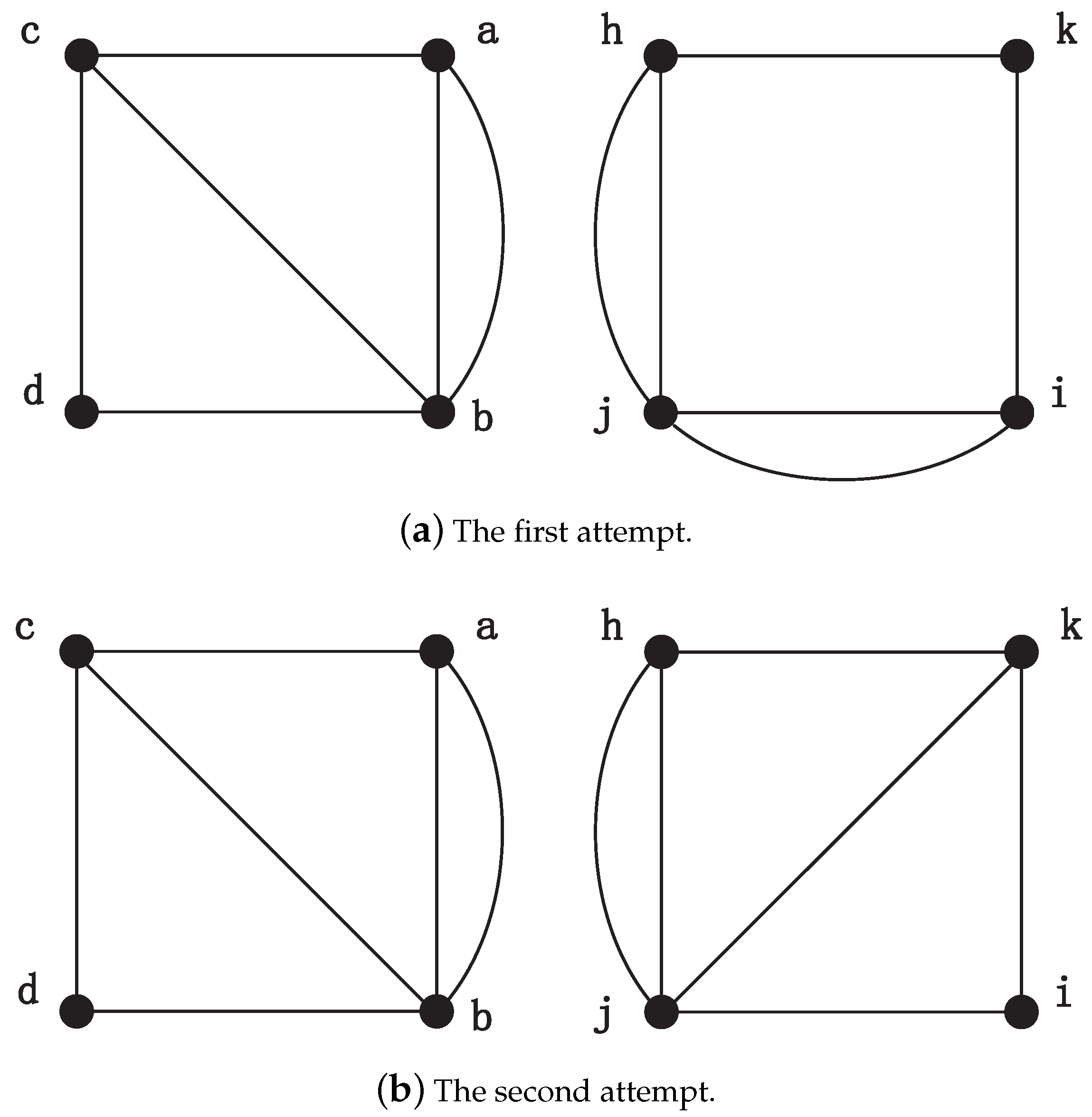
) are directly excluded from the candidates. Then, we choose vertex
j on the first attempt. Two new graphs are generated by adding auxiliary edges
and
, respectively, as shown in
Figure 5a. Since
c and
i are not matched in the new graphs by NodeMap, and node
i is rejected. When the candidate unit bijection
is considered, MapEff continues to add two auxiliary edges
and
, respectively. Hence, the new graphs are generated as shown in
Figure 5b. This time, these two graphs are isomorphic and the vertex
c can be mapped to
k in the NodeMap algorithm. As a result, the unit bijection
is accepted in the isomorphic mapping, and the new generated graph is maintained in the next iteration.
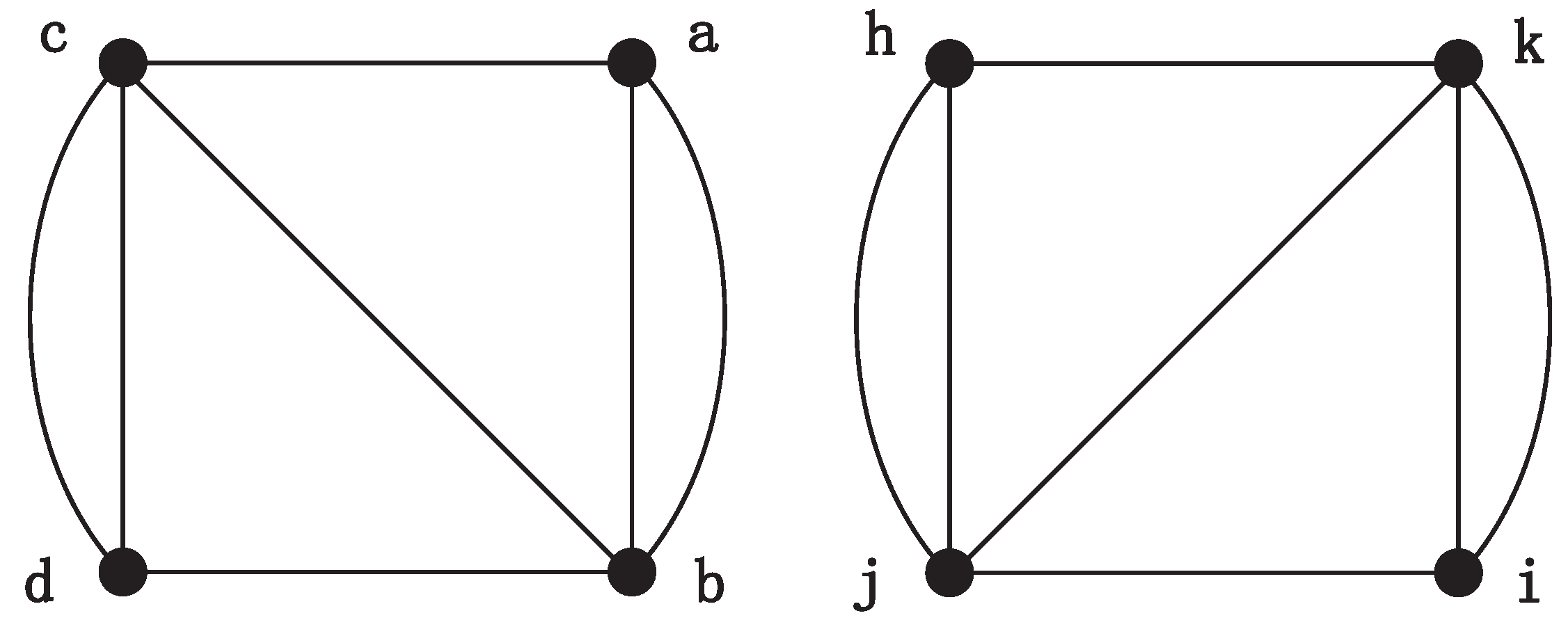
Finally, MapEff has to determine the mapping node of vertex d from its four candidates with the help of verified unit bijection . Because nodes h, j, and k conflict with a verified unit bijection, they are rejected. Therefore, there is only one node left to verify. When testing the candidate unit bijection , the vertex i can be a mapping node of d after performing the NodeMapp algorithm in the new graphs. Hence, MapEff accepts this unit bijection into the isomorphic mapping and outputs the final result .
Consequently, in this example, we can see that the unit bijection added into the isomorphic mapping one after another do not conflict with each other. The key point is equivalent nodes are distinguished by adding auxiliary edges. And the newly generated graphs, such as the graphs shown in
Figure 4,
Figure 5 and
Figure 6, also reduce the original symmetry. Although the square graph is highly symmetric and each node has the same number of neighbors, the addition of auxiliary edge is sufficient to distinguish the equivalent vertices. After multiple filters of candidate unit bijections, MapEff can discover a correct isomorphic mapping.
3.4. Algorithm Analysis
In this subsection, we discuss the computation complexity of our algorithm on two graphs, G and H, with the same number of vertices N.
According to the discussion in [
32], the computational complexity of simulating DTQW on the classical computer is
for the graph with
N nodes. Because the auxiliary graph constructed in Step 1 has
points, each simulation of DTQW in Step 1 costs
. In this step, this kind of operation is performed
times. Therefore, its computation complexity is
.
Next, we need to count the candidate matching nodes for each vertex in G. In the worst case, every vertex has N candidate matching nodes. So the complexity of Step 2 is .
When selecting the best candidate for each node in Step 3, we need to execute DTQW at most. Although the quantum walk we performed in this step is simulated on the auxiliary graph after adding extra edges, the computational complexity of each DTQW is still because the number of added edges is not greater than N. Therefore, the complexity of this step is .
After the above analysis, we can conclude that the computational complexity of this algorithm is .


