Nonadiabaticity in Quantum Pumping Phenomena under Relaxation

Abstract

The ability to control quanta shown by quantum pumping has been intensively studied, aiming to further develop nano fabrication. In accordance with the fast progress of the experimental techniques, the focus on quantum pumping extends to include the quicker transport. For this purpose, it is necessary to remove the “adiabatic” or “slow” condition, which has been the central concept of quantum pumping since its first proposal for a closed system. In this article, we review the studies which go beyond the conventional adiabatic approximation for open quantum systems to transfer energy quanta and electron spins with using the full counting statistics. We also discuss the recent developments of the nonadiabatic treatments of quantum pumping.

1. Introduction

According to the rapid development of experimental techniques, the downsizing of devices has been accelerated to extend possibilities to control single-electron current [1], spin-polarized current [2,3] and even thermal transport [4]. The trend is based on the aim to construct electronics with low energy consumption, quantum information processing, as well as quantum metrology [1,5].

Quantum pumping phenomena have attracted intensive attention, since they show the controllability of quantum transfer to extend the possibility of nano fabrications. The first proposal of quantum pumping was given by Thouless to transport electrons between two environments [6,7]. Its essential point is to adiabatically or slowly modulate the potential, which is described with the superposition of two standing waves in an out-of phase way [6,7,8]. Since the work of Thouless, the “adiabatic” change or “slow” modulation of parameters has played a central role in theoretical treatments of quantum pumping phenomena. However, the fast development of experimental techniques after the first experimental study on electron pumping with a quantum dot [9] requires us to investigate conditions on transferring quanta quicker and more precisely. In the present review, we classify the meaning of “quick” or “slow” in quantum pumping and show a standardized theoretical treatment—called full counting statistics (FCS)—to attain the purpose.

The physical situations referred to by the same term “adiabaticity” are roughly divided into three categories: (1) slow change in potential to allow the application of the adiabatic approximations to wave functions associated with transported particles [6,7]; (2) slow and small change of parameter(s) such as the chemical potential and voltage to allow a linear expansion of the scattering matrix [10,11,12,13,14,15,16,17] or Green functions [18,19,20,21,22,23,24,25,26] associated with transported electron charge or spin; and (3) slow change of parameters compared with the relaxation time of the relevant system with using FCS [27,28,29,30,31,32]. Different from the former two treatments, the third succeeds in including explicitly the finite relaxation time in adiabaticity. Because isolating any quantum system from its surroundings is impossible, considering relaxation phenomena is indispensable in implementing quantum pumping systems. With further developments of experimental techniques in mind, removing the adiabatic condition in this third instance is necessary. Before going further, let us provide a quick review of the conventional studies on pumping phenomena from the view point of the above summarized classifications of the adiabaticity.

Sinitsyn and Nemenman treated the classical two-state stochastic system [27] using FCS to represent the pumped quantity with a geometrical phase, first expounded in Reference [33]. The relationship between finite relaxation time and adiabaticity in the context of open quantum systems was first discussed by Ren, Hänggi, and Li [28] by extending the FCS approach in Reference [27]. Considering a two-level system coupled to two environments, they found that the pumping of energy quanta occurs under out-of-phase conditions and sufficiently slow (adiabatic) temperature modulations of the environments even if the bias is averaged out during a period. The power of the FCS approach can be found in the further application to electron charge pumping through single or double quantum dot(s) coupled to two leads [29,30,31]. They found that the sufficiently slow and out-of-phase modulations of the chemical potential can induce electron charge pumping, which is represented by a geometrical formula. In these instances, the condition for a sufficiently slow (adiabatic) environmental modulation means that the relevant two-level system approaches steady state sufficiently quickly.

In many varieties of quantum pumping phenomena, the generation of spin polarized electron current (spin current) by periodic parameter modulation has attracted a great deal of attention because of its promising applications in spintronics. Referred to as spin pumping, much effort has been made to develop its protocols. Conventionally, the protocols fall roughly into three classes: those using (i) a precession of magnetization in a magnetic material attached to a normal metal [12,13,19,20,21,22,23,24,25,26,34,35,36]; (ii) a periodic modulation of parameters such as gate voltages and/or tunneling amplitudes in a system consisting of quantum dots subjected to a magnetic field and normal metal leads [14,32,37,38,39,40]; and (iii) a periodic modulation of strength of magnetization in addition to parameters in a system consisting of quantum dots attached to a magnetic lead and/or normal metal leads [34,35,41,42]. Among these protocols, those using precession of magnetization—protocol (i)—have attracted intensive studies because it can generate pure spin current in a simple ferromagnet/normal metal heterojunction [3]. So far, the protocol has been mostly studied in situations where the precession of the magnetization is sufficiently slow, which is called adiabatic pumping. It was first proposed by Tserkovnyak et al. [12,13] based on the scattering theory of adiabatic quantum pumping given by Brouwer [11]. Its alternative formalisms based on Green’s function [19,20,22,23,24,25,26,36] have also been proposed by several authors. In these studies, the adiabatic contribution to the spin current generation has been obtained as a linear response to the precession, which corresponds to adiabaticity No. (2), with an implicit assumption of an infinite relaxation time. There are a few studies addressing adiabatic spin pumping with a finite relaxation time [34,35], where a slow modulation means smallness of the precession frequency comparing with the tunneling rate.

In the present article, we intend to review our recent studies on the role of nonadiabaticity with a finite relaxation time in quantum pumping of energy quanta and electron spins. For the purpose, we rely on adiabaticity condition No. (3), where the adiabaticity means a slow modulation of parameters compared to the relaxation time of the relevant system—defining the relaxation time of the relevant system as ${\tau }_r$, we find that the condition for a slow modulation requires ${\tau }_r$ to be much shorter than the period of the temperature modulation, which is written equivalently in terms of the modulation frequency $\mathsf{\Omega }$, ${\tau }_r^{-1}\gg \mathsf{\Omega }$. Thus, we consider the nonadiabatic regime up to ${\tau }_r^{-1}\gtrsim \mathsf{\Omega }$ in the following. As a formulation of nonadiabatic pumping, we present our extension of the FCS approach to quantum pumping toward the nonadiabatic regime. By applying the formulation to the pumping phenomena of energy quanta and electron spin, we find the following features: For the former, we demonstrate that nonadiabaticity yields a contribution to the pumped quantity in addition to the terms such as dynamical and geometrical phase terms which were obtained under adiabatic conditions. For the latter, surprisingly, we show that there are no contributions under the adiabatic condition and nonadiabaticity is an essential feature.

In the rest of the paper, we present in Section 2 our formulation describing the pumped quantity based on FCS. We discuss quantum heat pumping in Section 3 and spin pumping in Section 4, followed by a discussion and conclusion in Section 5.

2. General Formalism

We formulate a model of quantum pumping under periodic modulation of a parameter applying the FCS based on two-point projective measurements [43,44]. Let us consider a system consisting of a relevant system (S) and an environment (E) described by the Hamiltonian

$$H=H_0+H_{\mathrm{SE}},$$

(1)

where $H_0\equiv H_{\mathrm{S}}+H_{\mathrm{E}}$ and $H_{\mathrm{SE}}$ is the system–environment interaction. The FCS provides the statistical average of the net amount of a physical quantity, such as energy and particle number, exchanged between the system and the environment during a certain time interval. It is based on a joint probability of outcomes of two successive projective measurements of an observable of the environment Q corresponding to the exchanged quantity. The measurement scheme is—at $t=t_i$, we perform a projective measurement of Q to obtain a measurement outcome $q_{t_i}$; for $t_i\le t\le t_{i+1}$, the system undergoes a unitary time evolution through an interaction between the system and the environment; and at $t=t_{i+1}$, we perform a second projective measurement of Q to obtain another outcome $q_{t_{i+1}}$. The joint probability for the measurement scheme is given by

$$P[q_{t_{i+1}},q_{t_i}]\equiv \mathrm{Tr}[P_{q_{t_{i+1}}}U(t_{i+1},t_i)P_{q_{t_i}}W(t_i)P_{q_{t_i}}{U}^{†}(t_{i+1},t_i)P_{q_{t_{i+1}}}],$$

(2)

where $\mathrm{Tr}$ denotes the trace taken over the total system, $P_{q_t}\equiv |q_t⟩⟨q_t|$ the projective measurement of Q at t, $U(t,t_i)$ the unitary time evolution operator for the total system, and $W(t_i)$ the initial condition of the total system (see Note [45]). The net amount of exchanged quantity during the time interval $\delta t\equiv t_{i+1}-t_i$ is then given by $\Delta q_i\equiv q_{t_{i+1}}-q_{t_i}$, where its sign is chosen to be positive when the physical quantity is transferred from the system to the environment. The statistics of $\Delta q_i$ is contained in its probability distribution function

$$P(\Delta q_i)\equiv \sum _{q_{t_{i+1}},q_{t_i}}\delta (\Delta q_i-(q_{t_{i+1}}-q_{t_i}))P[q_{t_{i+1}},q_{t_i}],$$

(3)

The moments of $\Delta q_i$ are provided by the moment generating function,

$$Z(\lambda )\equiv {\int }_{-\infty }^{\infty }P(\Delta q_i)e^{i\lambda \Delta q_i}d\Delta q_i.$$

(4)

where $\lambda$ is the counting field associated with Q, for example, the mean value is computed from

$$⟨\Delta q_i⟩=\frac{\partial Z(\lambda )}{\partial (i\lambda )}{|}_{\lambda =0}.$$

(5)

Our next task is to describe the time evolution of $Z(\lambda )$. Using the Definition (3) and introducing the modified evolution operator $U_{\lambda }(t,t_i)\equiv e^{i\lambda Q}U(t,t_i)e^{-i\lambda Q}$, the moment generating function $Z(\lambda )$ is expressed as

$$Z(\lambda )=\mathrm{Tr}[W^{(\lambda )}(t_{i+1})],$$

(6)

with

$$W^{(\lambda )}(t)\equiv U_{\lambda /2}(t,t_i)\overline{W}(t_i)U_{-\lambda /2}^{†}(t,t_i),$$

(7)

where $\overline{W}(t_i)\equiv {\sum }_{q_{t_i}}{P}_{q_{t_i}}W(t_i)P_{q_{t_i}}$ is the diagonal part of $W(t_i)$. For $\lambda =0$, $W^{(\lambda =0)}(t)$ reduces to the usual reduced density matrix of the total system. By taking the time derivative of $W^{(\lambda )}(t)$, we obtain a modified Liouville–von Neumann equation

$$i\frac{\partial }{\partial t}{W}^{(\lambda )}(t)={\mathcal{L}}^{(\lambda )}{W}^{(\lambda )}(t),$$

(8)

with a modified Liouvillian ${\mathcal{L}}^{(\lambda )}{W}^{(\lambda )}(t)\equiv {\hslash }^{-1}{[H,W^{(\lambda )}(t)]}_{\lambda }$, where ${[A,B]}_{\lambda }\equiv A^{(\lambda )}B-B{A}^{(-\lambda )}$, and $A^{(\lambda )}\equiv e^{i\lambda Q/2}A{e}^{-i\lambda Q/2}$. In Appendix B, we explain the connection between the formalism of the FCS based on two-point measurements and the formalism by Sinitsyn and Nemenman in Reference [27].

By introducing a projection operator $\mathcal{P}:W^{(\lambda )}(t)\mapsto {\mathrm{Tr}}_{\mathrm{E}}[W^{(\lambda )}(t)]\otimes {\rho }_{\mathrm{E}}$, where ${\mathrm{Tr}}_{\mathrm{E}}$ is the partial trace taken over the environment and ${\rho }_{\mathrm{E}}$ is a fixed state of the environment, the equation of motion for the reduced operator of the relevant system ${\rho }^{(\lambda )}(t)\equiv {\mathrm{Tr}}_{\mathrm{E}}[W^{(\lambda )}(t)]$ can be cast into the form of a time convolutionless (TCL)-type quantum master equation [46,47,48,49,50,51,52,53].

Assuming that the initial state is factorized between system and environment as $W(t_i)=\rho (t_i)\otimes {\rho }_{\mathrm{E}}$ and the fixed state of the environment ${\rho }_{\mathrm{E}}$ is the Gibbs state with an inverse temperature $\beta$, the TCL master equation including the counting field is expressed as

$$\frac{\partial }{\partial t}{\rho }^{(\lambda )}(t)={\xi }^{(\lambda )}(t){\rho }^{(\lambda )}(t).$$

(9)

The super-operator ${\xi }^{(\lambda )}(t)$ is expanded as a sum of “ordered cumulants” of the interaction Hamiltonian $H_{\mathrm{SE}}$ up to infinite order. Taking leading terms up to second-order, we have

$${\xi }^{(\lambda )}(t){\rho }^{(\lambda )}(t)=-\frac{i}{\hslash }[H_{\mathrm{S}},{\rho }^{(\lambda )}(t)]-\frac{1}{{\hslash }^2}{\int }_0^{t}d\tau {\mathrm{Tr}}_{\mathrm{E}}{[H_{\mathrm{SE}},{[H_{\mathrm{SE}}(-\tau ),{\rho }^{(\lambda )}(t)\otimes {\rho }_{\mathrm{E}}^{\mathrm{eq}}]}_{\lambda }]}_{\lambda }.$$

(10)

Note that the time dependence of the memory kernel reflects the finiteness of the correlation time of the dot–lead interaction, which allows us to describe the non-Markovian dynamics.

To work with the super-operator, it is convenient to introduce its supermatrix representation, where we represent the density matrix ${\rho }^{(\lambda )}$ in vector form and the super-operator ${\xi }^{(\lambda )}$ in matrix form. In this representation, the formal solution of the master equation Equation (9) is expressed as

$$|{\rho }^{(\lambda )}(t)⟩⟩={\mathrm{T}}_{+}exp\left[{\int }_{t_i}^t{\Xi }^{(\lambda )}(s)ds\right]|{\rho }^{(\lambda )}(t_i)⟩⟩,$$

(11)

where $|{\rho }^{(\lambda )}(t)⟩⟩$ represents the vector form of ${\rho }^{(\lambda )}(t)$, ${\mathrm{T}}_{+}exp$ the time-ordered exponential, and ${\Xi }^{(\lambda )}(t)$ the supermatrix form of ${\xi }^{(\lambda )}(s)$. With the representation, the moment generating function Equation (6) is rewritten as $Z(\lambda )={\mathrm{Tr}}_{\mathrm{S}}[{\rho }^{(\lambda )}(t_{i+1})]=⟨⟨1|{\rho }^{(\lambda )}(t_{i+1})⟩⟩$, where ${\mathrm{Tr}}_{\mathrm{S}}$ is the partial trace taken over the relevant system and $⟨⟨1|$ the vector representation of the partial trace ${\mathrm{Tr}}_{\mathrm{S}}$. Using the formal solution Equation (11), we recast the expression of the mean value into the form

$$⟨\Delta q_i⟩={\int }_{t_i}^{t_{i+1}}J(s)ds$$

(12)

with the inertial flow of the quantity,

$$J(t)\equiv ⟨⟨1|[\frac{\partial {\Xi }^{(\lambda )}(t)}{\partial (i\lambda )}{]}_{\lambda =0}|{\rho }^{(\lambda =0)}(t)⟩⟩.$$

(13)

To formulate quantum pumping based on the above framework, we need to accumulate transfers of the physical quantity under a cyclic modulation of system and/or environmental parameters during a period $\mathcal{T}$. For this purpose, we consider a step-like change of the parameters; specifically, dividing the period $\mathcal{T}$ into N intervals, $t_i\le t\le t_{i+1}$ ($i=1,2,\cdots ,N$) with $t_1=0$ and $t_{N+1}=\mathcal{T}$, fixing a value of the parameters during each interval, and changing the value at each $t_i$ discretely. With the total density matrix factorized at each $t_i$, the mean value as well as the inertial flow of the quantity for each interval are given by Equations (12) and (13), respectively. The time integration of $J(t)$ over one period $\mathcal{T}$ provides the accumulated value of the quantity over one cycle

$$⟨\Delta q⟩\equiv {\int }_0^{\mathcal{T}}J(t)dt=\sum _{i=1}^N⟨\Delta q_i⟩,$$

(14)

where $⟨\Delta q_i⟩$ is the mean value of the net transferred quantity in the ith interval.

3. Pumping of Energy Quanta

3.1. Model

Let us consider the energy transfer via a two-level system between two environmental systems (L and R) consisting of an infinite number of bosons [28,54,55,56]. With the definition of the lower (higher) level of the two-level system as $|0⟩$ ($|1⟩$), respectively, the Hamiltonian of the model is written as

$$\begin{array}{ccc}\hfill H_{\mathrm{S}}& =& \sum _{m=0,1}{\epsilon }_m|m⟩⟨m|,H_{\mathrm{E}}=\sum _{k,\nu }\hslash {\omega }_{k,\nu }{b}_{k,\nu }^{†}{b}_{k,\nu },\hfill \\ \hfill H_{SE}& =& \sum _{\nu }{X}_{\nu }(|0⟩⟨1|+|1⟩⟨0|),(\nu =L,R),\hfill \end{array}$$

(15)

where $X_{\nu }={\sum }_k\hslash g_{k,\nu }(b_{k,\nu }^{†}+b_{k,\nu })$, with $b_{k,\nu }^{†}$ and $b_{k,\nu }$ the creation and annihilation boson operators of the kth mode of the $\nu$th environment. The model scheme is shown in Figure 1A.

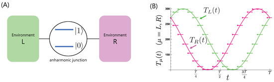
Figure 1. (A) Model scheme: a two-level system as an anharmonic junction interacts with two environments (L and R). (B) Temperature modulations, $T_L(t)=200+100cos(\omega t+\pi /4)$, and $T_R(t)=200+100sin(\omega t+\pi /4)$, discretized with $N=20$.

We consider the energy transfer from out-of-phase temperature modulations of the two environments, corresponding to the bias averaged out during a period $\mathcal{T}$ [28]. To discuss the nonadiabaticity for this model, we study energy (boson) transfers under cyclic and piecewise modulations of the environmental temperatures $T_L$ and $T_R$ dividing $\mathcal{T}$ into N intervals, $t_i\le t\le t_{i+1}$$(i=1,\cdots ,N)$ with $t_1=0$ and $t_{N+1}=\mathcal{T}$. We need to discretize the temperature modulation because conventional treatments describing relaxation phenomena require the environmental temperature to remain constant. By changing the number of intervals of the temperature modulation, we compared each time interval with the relaxation time of the relevant two-level system and thus we are able to discuss nonadiabaticity explicitly, for example, from the scale between ${\tau }_r^{-1}$ and $\mathsf{\Omega }$. In taking the limit $N\to \infty$, we reveal energy transfer features under a continuous modulation. In Figure 1B, we plot the time dependence of the temperature modulations used in this study calculated for a typical number of discrete time intervals $N=20$.

3.2. FCS Formalism Applied to Pumping of Energy Quanta

We apply the general formalism of the FCS in the former section to this model focusing on weak system–environment coupling and considering long time (Born-Markovian) limits by taking $t\to \infty$ in the upper bound of the integral in Equation (10). In this limit, the super-operator ${\xi }^{(\lambda )}(t)$ becomes time independent during each interval. We find that the mean value of the transferred quantity between the relevant two-level system and the $\nu$th environment in the ith time interval, $⟨\Delta q_i^{\nu }⟩$ is written as

$$\begin{array}{c}\hfill ⟨\Delta q_i^{\nu }⟩=\hslash {\omega }_0\{A_i^{\nu }{\int }_{t_i}^{t_{i+1}}d{t}^{\prime }{\rho }_{00}(t^{\prime })-B_i^{\nu }\delta t\},\end{array}$$

(16)

with ${\omega }_0=({\epsilon }_1-{\epsilon }_0)/\hslash$, ${\rho }_{00}(t)=⟨0|{\rho }^{(\lambda =0)}(t)|0⟩$, and $\delta t=t_{i+1}-t_i$. $A_i^{\nu }$ and $B_i^{\nu }$ in Equation (16) are coefficients defined as $A_i^{\nu }=-(k_{d,i}^{\nu }+k_{u,i}^{\nu })$ and $B_i^{\nu }=-k_{u,i}^{\nu }$ with rate constants $k_{u,i}^{\nu }$ and $k_{d,i}^{\nu }$, which govern the time evolution of ${\rho }_{00}(t)$ during $t_{i-1}\le t<t_i$. Their explicit expressions are $k_{d,i}^{\nu }={\Gamma }_{\nu }{n}_{\nu ,i}$ and $k_{u,i}^{\nu }={\Gamma }_{\nu }(1+n_{\nu ,i})$, where $n_{\nu ,i}=1/(exp[\hslash {\beta }_i^{\nu }{\omega }_0]-1)$ is the Bose–Einstein distribution for the inverse temperature ${\beta }_i^{\nu }$ of the $\nu$th environment during the ith interval and ${\Gamma }_{\nu }$ denotes the feature of the system–environment coupling as ${\Gamma }_{\nu }=2\pi h_{\nu }({\omega }_0)$ with the coupling spectral density $h_{\nu }(\omega )\equiv {\sum }_k{g}_{k,\nu }^2\delta (\omega -{\omega }_{k,\nu })=\lambda \omega exp[-\omega /{\omega }_c]$, where $\lambda$ is the coupling strength and ${\omega }_c$ is the cutoff frequency. To obtain $⟨\Delta q_i^{\nu }⟩$, we need ${\rho }_{00}(t)$, the time evolution for which is

$$\begin{array}{c}\hfill {\dot{\rho }}_{00}(t)=-K_{d,i}{\rho }_{00}(t)+K_{u,i}{\rho }_{11}(t)\end{array}$$

with $K_{d,i}={\sum }_{\nu }{k}_{d,i}^{\nu }$ and $K_{u,i}={\sum }_{\nu }{k}_{u,i}^{\nu }$. The differential equation for ${\rho }_{00}(t)$ is solved to give

$$\begin{array}{c}\hfill {\rho }_{00}(t)={\rho }_{s,i}+e^{{\Lambda }_{i}t}({\rho }_{00}(t_{i-1})-{\rho }_{s,i}),\end{array}$$

(17)

where we denote ${\rho }_{s,i}=-K_{u,i}/{\Lambda }_i$ with ${\Lambda }_i=-(K_{d,i}+K_{u,i})$. Using Equations (12), we find that the total transferred energy during the period is calculated to be

$$\begin{array}{c}\hfill ⟨\Delta q^{\nu }⟩=\sum _{i=1}^{N+1}⟨\Delta q_i^{\nu }⟩=\hslash {\omega }_0({\mathcal{G}}_1^{\nu }+{\mathcal{G}}_2^{\nu }+{\mathcal{G}}_3^{\nu }),\end{array}$$

(18)

where

$$\begin{array}{ccc}\hfill {\mathcal{G}}_1^{\nu }& =& \sum _{i=1}^{N+1}(A_i^{\nu }{\rho }_{s,i}-B_i^{\nu })\delta t,\hfill \end{array}$$

(19)

$$\begin{array}{ccc}\hfill {\mathcal{G}}_2^{\nu }& =& \sum _{i=1}^N\frac{A_{i+1}^{\nu }}{{\Lambda }_{i+1}}({\rho }_{s,i+1}-{\rho }_{s,i}),\hfill \end{array}$$

(20)

$$\begin{array}{ccc}\hfill {\mathcal{G}}_3^{\nu }& =& \sum _{i=1}^{N+1}{\varphi }_{0,i}^{\nu }+\sum _{i=2}^N({\rho }_{s,i-1}-{\rho }_{s,i}){\psi }_i^{\nu }+({\rho }_{s,n-1}-{\rho }_{s,n})\frac{A_n^{\nu }}{{\Lambda }_n}{e}^{{\Lambda }_n\delta t},\hfill \end{array}$$

(21)

with

$$\begin{array}{ccc}\hfill {\varphi }_{0,i}^{\nu }& =& ({\rho }_{00}(0)-{\rho }_{s,1})f^{\nu }(1,i),\hfill \end{array}$$

(22)

$$\begin{array}{ccc}\hfill {\psi }_i^{\nu }& =& \frac{A_i^{\nu }}{{\Lambda }_i}{e}^{{\Lambda }_i\delta t}+\sum _{m=i}^N{f}^{\nu }(i,m+1),\hfill \end{array}$$

(23)

$$\begin{array}{ccc}\hfill f^{\nu }(p,q)& =& \frac{A_q^{\nu }}{{\Lambda }_q}{e}^{{\sum }_{\kappa =p}^{q-1}{\Lambda }_{\kappa }\delta t}(e^{{\Lambda }_q\delta t}-1).\hfill \end{array}$$

(24)

In the next subsection, we show the physical meanings of these obtained terms.

3.3. Adiabatic and Nonadiabatic Contributions

Taking the Riemann sum on ${\mathcal{G}}_1^{\nu }$ and ${\mathcal{G}}_2^{\nu }$ by setting $N\to \infty$ and $\delta t\to 0$, we find that they reduce to the dynamical and geometrical phases, respectively. For instance, we obtain the energy transfer with the environment R with setting $\nu =R$ as [56]

$${\mathcal{G}}_1^R={\int }_0^{\mathcal{T}}d{t}^{\prime }\frac{{\Gamma }_L{\Gamma }_R(n_L(t^{\prime })-n_R(t^{\prime }))}{K},$$

(25)

with $K\equiv {\sum }_{\nu =L,R}{\Gamma }_{\nu }(1+2n_{\nu }(t^{\prime }))$, and

$${\mathcal{G}}_2^R=\int \int d{T}_{L}d{T}_R\left\{\frac{2{\Gamma }_L{\Gamma }_R({\Gamma }_L+{\Gamma }_R)}{K^3}\frac{d{n}_R}{d{T}_R}\frac{d{n}_L}{d{T}_L}\right\},$$

(26)

which coincide with the ones in Reference [28] and imply that the sum of ${\mathcal{G}}_1^{\nu }$ and ${\mathcal{G}}_2^{\nu }$ corresponds to the adiabatic contribution.

Considering this point, we find that the nonadiabatic contribution is described with a new extra term in $⟨\Delta q^{\nu }⟩$ added to the adiabatic contribution in the form,

$$\begin{array}{c}\hfill ⟨\Delta q^{\nu }⟩={\mathcal{G}}_{ad}^{\nu }+{\mathcal{G}}_{nad}^{\nu },\end{array}$$

(27)

with ${\mathcal{G}}_{ad}^{\nu }={\mathcal{G}}_1^{\nu }+{\mathcal{G}}_2^{\nu }$ and ${\mathcal{G}}_{nad}^{\nu }={\mathcal{G}}_3^{\nu }$. This is consistent with the expression of ${\mathcal{G}}_3^{\nu }$, which shows that, when ${\rho }_{00}(0)={\rho }_{s,1}$ and the absolute value of ${\Lambda }_i\delta t$ is sufficiently large, we can neglect ${\mathcal{G}}_3^{\nu }$. The former condition corresponds to the adiabatic approximation in Reference [28], where the population of the relevant system instantaneously approaches the steady state for the temperature setting at an initial time. The term ${\mathcal{G}}_3^{\nu }$ shows that the nonadiabatic contribution to the transferred quantity explicitly depends on the initial condition of the relevant system, ${\rho }_{00}(0)$. Moreover, expanding Equation (13) about $\delta t$ up to the first order, we find that the nonadiabatic effect described in ${\mathcal{G}}_3^{\nu }$ shows a correction to both ${\mathcal{G}}_1^{\nu }$ and ${\mathcal{G}}_2^{\nu }$. In the following, we present a numerical evaluation of the formulas obtained.

3.4. Numerical Evaluation of the Nonadiabatic Spin Pumping

3.4.1. Population Dynamics

Figure 2 presents the transient time evolution of ${\rho }_{00}(t)$ during the first period of modulation by changing the time interval $\delta t$ while keeping the number of divisions N constant at $N=40$. We set parameters as $\lambda =0.01$, ${\omega }_c=3{\omega }_0$, and $\hslash {\omega }_0=25$ meV which shows the relaxation time ${\overline{\tau }}_r\equiv {\omega }_0{\tau }_r\approx 5$. (The value of $\hslash {\omega }_0$ is chosen to be the same as the typical value for a molecular junction in Reference [28].) Setting the initial condition of the two-level system with the effective inverse temperature as ${\overline{\beta }}_s=\frac{\hslash {\omega }_0}{k_B{T}_s}=\overline{\beta }(0)(\approx 1.07)$ corresponding to the stationary state for the initial temperature setting, we plot the time dependence of the population in the lower state, ${\rho }_{00}(t)$. The population ${\rho }_{00}(t)$ under the adiabatic approximation (Figure 2, red line) shows that the relevant system quickly approaches the stationary state corresponding to the temperature setting in each time interval. Setting the interval $\delta t$ to be much larger than the relaxation time as in Figure 2A corresponding to the lower modulation frequency $\mathsf{\Omega }=0.3$ THz, we find that the relevant system mostly follows the temperature modulation as the stationary state is approached, which shows the feature close to the adiabatic approximation. With decreasing interval $\delta t$ (Figure 2B,C), we find that the relevant system does not follow the temperature modulation thus exhibiting nonadiabaticity.

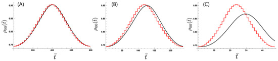
Figure 2. Time dependence of the population in the lower state of the two-level system with changing modulation frequency: (A) $\mathsf{\Omega }=0.3\mathrm{THz}$, (B) $\mathsf{\Omega }=1\mathrm{THz}$, and (C) $\mathsf{\Omega }=5\mathrm{THz}$ with $s=0.01$, ${\omega }_c=3{\omega }_0$, $\hslash {\omega }_0=25\mathrm{meV}$, and $N=40$. The time variable is scaled with ${\omega }_0$ as $\overline{t}={\omega }_{0}t$.

3.4.2. Frequency Dependence

We show in Figure 3 the frequency dependence of the pumped quantity ${\widehat{I}}_{\mathrm{energy}}=\frac{1}{\mathcal{T}\hslash {\omega }_0}(⟨\Delta q^R⟩-⟨\Delta q^L⟩)$. For comparison, we also exhibit the frequency dependence of the quantity under the adiabatic approximation presented as a geometric phase in Reference [28]. We find that the nonadiabatic term decreases the pumped quantity in the higher frequency region. We also find that the pumped quantity depends on the initial condition of the two-level system. The feature shown in Figure 3 is universal for different settings of these parameters. For example, when we increase ${\tau }_r$ by decreasing the coupling strength with keeping the value of ${\omega }_0$, we find the similar feature of the frequency dependence ranging up to ∼10 GHz which corresponds to the maximum driving frequency of electronic voltage due to the limitation of experimental bandwidth at the present time. The parameter setting of $\lambda$ in this study is chosen to expect the further acceleration of the recent rapid development of Tera Hz technology in a future.

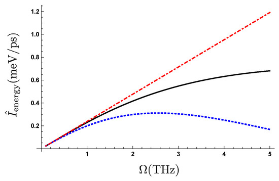
Figure 3. (Color online) Frequency dependence of pumped quantity $I_{\mathrm{energy}}$ with $\lambda =0.01$, ${\omega }_c=3{\omega }_0$, and $\hslash {\omega }_0=25\mathrm{meV}$ with changing initial conditions of the two-level system ${\overline{\beta }}_s$ values: (1) the black line corresponds to ${\overline{\beta }}_s=\overline{\beta }(0)(\approx 1.07)$ which is the effective inverse temperature of the stationary state for the initial temperature setting, (2) the blue dotted line to ${\overline{\beta }}_s=5$; (3) the red dottdashed line represents the frequency dependence of the net geometrical phase [28].

4. Spin Pumping

4.1. A Minimum Model of Spin Pumping

We consider a minimum model of spin pumping involving a quantum dot with dynamic magnetization and an electron lead (Figure 4A). The magnetization of the dot $\mathit{M}(t)$ rotates around the z-axis with a period $\mathcal{T}$. An electron in the quantum dot is spin polarized because of the s–d exchange interaction with magnetization and is represented by the two-component creation and annihilation operators ${\mathit{d}}^{†}=(d_{\uparrow }^{†},d_{\downarrow }^{†})$, and $\mathit{d}$, where ↑ and ↓ denote the direction of the electron’s spin magnetic moment parallel and antiparallel, respectively, to the z-axis.

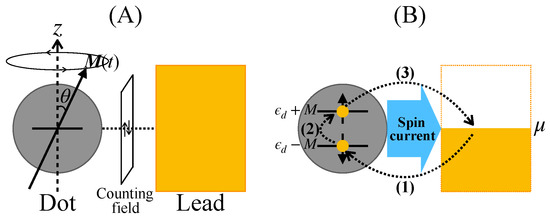
Figure 4. (A) The minimum model consists of a ferromagnetic quantum dot attached to an electron lead. The dot has a dynamic magnetization $\mathit{M}(t)$ that rotates around the z-axis with a period $\mathcal{T}$. The number of transferred electrons with spin magnetic moment ↑ (↓) is captured by the counting field. (B) Schematic of the spin current generation in the minimum model. The scheme can be summarized as follows: (1) an electron with ↓-spin enters from the lead onto the dot subject to the dot–lead interaction; (2) the spin of the electron is flipped by the precessing magnetization; (3) the electron with ↑-spin moves back from the dot to the lead.

The Hamiltonian of the minimum model consists of three terms $H(t)=H_{\mathrm{d}}(t)+H_{\mathrm{l}}+H_{\mathrm{t}}$. $H_{\mathrm{d}}(t)$, describing the dot, is defined by

$$H_{\mathrm{d}}(t)={\mathit{d}}^{†}[{ϵ}_{\mathrm{d}}-\mathit{M}(t)·\mathit{\sigma }]\mathit{d},$$

(28)

where ${ϵ}_{\mathrm{d}}$ is the unpolarized energy of a dot electron, $\mathit{M}(t)\equiv M(sin\theta sin\varphi (t),sin\theta sin\varphi (t),cos\theta )$, and $\mathit{\sigma }=({\sigma }_x,{\sigma }_y,{\sigma }_z)$ the vector of Pauli matrices. Introducing the eigenstates $|j_{\uparrow },j_{\downarrow }⟩$ (with $j_{\uparrow (\downarrow )}=0$ or 1) of the number operator of the dot electron ${\sum }_{\sigma }{d}_{\sigma }^{†}{d}_{\sigma }$ as a basis, the dot Hamiltonian is represented by the matrix

$$\begin{array}{cc}& \begin{array}{cccc}|0,0⟩\begin{array}{cc}& \end{array}& |0,1⟩\begin{array}{ccc}& & \end{array}& \begin{array}{ccc}& & \end{array}|1,0⟩& \begin{array}{ccc}& & \end{array}|1,1⟩\end{array}\\ H_{\mathrm{d}}(t)=& \left(\begin{array}{cccc}0& 0& 0& 0\\ 0& {ϵ}_{\mathrm{d}}+Mcos\theta & -M{e}^{+i\varphi (t)}sin\theta & 0\\ 0& -M{e}^{-i\varphi (t)}sin\theta & {ϵ}_{\mathrm{d}}-Mcos\theta & 0\\ 0& 0& 0& 2{ϵ}_{\mathrm{d}}\end{array}\right)\end{array}.$$

(29)

The electron lead is described by the term

$$H_{\mathrm{l}}=\sum _{\sigma =\uparrow ,\downarrow }\sum _k{ϵ}_k{c}_{\sigma ,k}^{†}{c}_{\sigma ,k},$$

(30)

where $c_{\sigma ,k}$ and $c_{\sigma ,k}^{†}$ with $\sigma =\uparrow$ or ↓ are annihilation and creation operators of a lead electron with energy ${ϵ}_k$ and spin-$\sigma$. The dot–lead interaction is assumed to be spin conserving with

$$H_{\mathrm{t}}=\sum _{\sigma }\sum _k\hslash v_k(d_{\sigma }^{†}{c}_{\sigma ,k}+c_{\sigma ,k}^{†}{d}_{\sigma }),$$

(31)

where $\hslash v_k$ is the coupling strength, which we assume to be weak.

Intuitively, the generation of the spin current in the minimum model is summarized by the following scheme (see Figure 4B): (1) an electron with ↓-spin moves from lead to dot under the dot–lead interaction, (2) the spin of the electron is flipped by the precessing magnetization, and (3) an electron with ↑-spin moves back from dot to lead. For spin-current generation, the essential conditions required in setting parameter values are

$${ϵ}_{\mathrm{d}}-M<\mu <{ϵ}_{\mathrm{d}}+M\mathrm{and}{\beta }^{-1}\le 2M,$$

(32)

where $\beta$ is the inverse temperature of the lead.

4.2. FCS Formalism of the Spin Pumping

In the following, we apply the FCS outlined in Section 2 to evaluate the number of transferred electrons with spin $\sigma$ from projective measurements of the electron number in the lead represented by $N_{\sigma }\equiv {\sum }_k{c}_{\sigma ,k}^{†}{c}_{\sigma ,k}$. By associating $H_{\mathrm{d}}(t)$, $H_{\mathrm{l}}$, and $H_{\mathrm{t}}$ with $H_{\mathrm{S}}$, $H_{\mathrm{E}}$, and $H_{\mathrm{SE}}$, respectively, and defining an outcome of the projective measurement at time t as $n_{\sigma ,t}$, we analyze the electron dynamics under spin pumping.

In order to explicitly examine the influence of the relaxation process on the spin current generation, we discretize the rotation of $\mathit{M}(t)$: divide the period $\mathcal{T}$ into N intervals, $t_i\le t\le t_{i+1}$$(i=1,\cdots ,\mathrm{N})$ with $t_1=0$ and $t_{N+1}=\mathcal{T}$; fix the direction of $\mathit{M}(t)$ during each interval; and change $\varphi$ at each $t_i$ discretely with substitution ${\varphi }_i={\varphi }_{i-1}+\delta \varphi$ with ${\varphi }_0=0$, ${\varphi }_N=2\pi$ and $\delta \varphi \equiv 2\pi /N$ (see Note [57]). The net number of electrons with spin-$\sigma$ during the ith interval can be evaluated from the difference in outcomes $\Delta n_{\sigma ,i}=n_{\sigma ,t_{i+1}}-n_{\sigma ,t_i}$.

By introducing counting fields ${\lambda }_{\uparrow }$ and ${\lambda }_{\downarrow }$ corresponding to observables $N_{\uparrow }$ and $N_{\downarrow }$, respectively, we can evaluate the mean value of transferred electrons,

$$⟨\Delta n_{\uparrow (\downarrow ),i}⟩={\int }_{t_i}^{t_{i+1}}{J}_{\uparrow (\downarrow )}(t),$$

(33)

with an inertial flow of electrons

$$J_{\uparrow (\downarrow )}(t)\equiv ⟨⟨1|[\frac{\partial {\Xi }^{({\lambda }_{\uparrow (\downarrow )})}(t)}{\partial (i{\lambda }_{\uparrow (\downarrow )})}{]}_{{\lambda }_{\uparrow (\downarrow )}=0}|{\rho }^{({\lambda }_{\uparrow (\downarrow )}=0)}(t)⟩⟩.$$

(34)

The inertial flow of electrons provides an instantaneous spin current,

$$J_{\mathrm{spin}}(t)\equiv J_{\uparrow }(t)-J_{\downarrow }(t),$$

(35)

and its time integration over one period provides a temporal average of the spin current,

$$I_{\mathrm{spin}}\equiv \frac{1}{\mathcal{T}}{\int }_0^{\mathcal{T}}{J}_{\mathrm{spin}}(t)dt.$$

(36)

To discuss the role of nonadiabaticity in spin pumping, we focus the Born-Markovian (long-time) limit by taking the limit $t\to \infty$ of the supermatrix ${\Xi }^{(\lambda )}(t)$ in each interval. In this limit, the matrix elements of ${\Xi }^{(\lambda )}$ are time-independent during each interval and determined by the direction of $\mathit{M}$ in each interval.

4.3. Absence of Adiabatic Contribution

Let us first show absence of the adiabatic contribution to the spin pumping in the minimum model. In previous studies, the adiabatic regime of the spin pumping in the minimum model has been studied based on the linear expansion of the Green function in the rotation frequency of $\mathit{M}(t)$ [23,24], which we referred to as the adiabaticity No. (2). The purpose of the present subsection is to re-examine the adiabatic contribution of the spin pumping from the view point of the adiabaticity No. (3), where we consider a sufficiently slow rotation of $\mathit{M}(t)$ comparing to the relaxation time, that is, $\mathsf{\Omega }\ll {\tau }_r^{-1}$ following the procedure by Sinitsyn and Nemenman in Reference [27].

Following the procedure, the adiabatic regime is assessed by dividing the cycle of modulation into time intervals $\delta t(\equiv \mathcal{T}/N)$ and assuming a quick approach of the system to its steady state in each interval. In the steady state of the minimum model, we can expect that the quantum dot is occupied by a single electron whose spin is aligned toward the direction of $\mathit{M}(t)$, and, because of the rotational symmetry of the model, the steady state populations of the quantum dot are invariant under the rotation of $\mathit{M}(t)$ around the z-axis. It indicates that no electron transfer occurs in the adiabatic regime. As a result, we can expect absence of the adiabatic contribution to the spin current generation. We provide an analytical proof of the intuitive observation in Appendix C (see also the original argument in Section 4 in Reference [58]).

As a result, we need to include the nonadiabatic effect to obtain a finite spin current. It is in marked contrast to the previous example of the energy pumping, where the adiabatic contribution to the energy pumping ${\mathcal{G}}_{ad}^{\nu }$ is finite.

4.4. Numerical Evaluation of the Nonadiabatic Spin Pumping

We now turn to examine nonadiabaticity in spin pumping. For this purpose, we evaluate numerically the instantaneous spin current $J_{\mathrm{spin}}(t)$ and its temporal average $I_{\mathrm{spin}}$.

To describe the dot–lead coupling, we use the Ohmic spectral density with an exponential cutoff $v(\omega )\equiv {\sum }_k{v}_k^2\delta (\omega -{\omega }_k)=\lambda \omega exp[-\omega /{\omega }_c]$, where $\lambda$ is the coupling strength and ${\omega }_c$ is the cutoff frequency. For the numerical calculation, we chose $2M$, the energy difference between the spin-↑ and -↓ states in the dot, as an energy unit. We distinguish parameters normalized by their units using an overbar (see Note [59]). Specific values of the normalized parameters are given in the figure captions. As we are focusing on the spin transfer driven by the rotating magnetization, the dot is set in a steady state Equation (A25) at $\overline{t}=0$ to exclude any transient spin transfer caused by the dot–lead contact.

4.4.1. Electron Transfer Dynamics

Let us first examine electron transfer dynamics under the cyclic rotation of the magnetization to show the generation of the spin current in the nonadiabatic regime. For this purpose, we numerically evaluate the time evolution of the populations ${\rho }_{j{j}^{\prime }}(t)=⟨j,j^{\prime }|{\rho }^{(0)}(t)|j,j^{\prime }⟩$ (${\rho }_{00}$: empty state, ${\rho }_{10}$: half-filled state with spin-↑, ${\rho }_{01}$: half-filled state with spin-↓, and ${\rho }_{11}$: completely filled state) and corresponding instantaneous electron and spin currents, $J_{\uparrow (\downarrow )}(t)$ and $J_{\mathrm{spin}}(t)$. In Figure 5A,B, we present the time evolution of populations and instantaneous currents for one cycle of the step-like rotation with division number $N=5$ and time interval $\delta t=20$. The change in angle at each subsequent $t_i$ is $\delta \varphi =2\pi /5$, that is ${\varphi }_i={\varphi }_{i-1}+2\pi /5$ with ${\varphi }_0=0$.

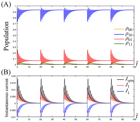
Figure 5. (A) Time evolution of the populations in the dot under the step-like precession of the magnetization with $\delta \overline{t}=20$ and $N=5$. The populations deviate from their steady-state values just after a sudden change of the angle $\varphi$, but then they approach new steady state-values for each ${\varphi }_i$. The figure shows the steady-state values of the populations to be invariant. This is because of the rotational symmetry of the system about the z-axis. (B) The instantaneous electron and spin currents $J_{\uparrow }(t)$ (red line), $J_{\downarrow }(t)$ (blue line) and $J_{\mathrm{spin}}(t)$ (black line) corresponding to the population dynamics in panel (A). The time dependences of the instantaneous currents indicate that electrons starts moving between dot and lead just after the sudden change of $\varphi$, and $J_{\uparrow }$ and $J_{\downarrow }$ have opposing directions. The latter trend show that the instantaneous electron currents are balanced as a result of charge conservation in the lead. In contrast, the instantaneous spin current $J_{\mathrm{spin}}$ always takes positive values indicating constant spin current generation. The parameters are set to ${\overline{ϵ}}_{\mathrm{d}}=10$, $\overline{\mu }=10$, $\overline{\beta }=100$, $\lambda =0.01$, ${\overline{\omega }}_c=4$, $\theta =5\pi /6$, and $\delta \varphi =2\pi /5$, which satisfies the condition (32).

In Figure 5A, we find that initially the populations deviate from their steady-state values by changing $\varphi$ at $t_i$, but then they approach new steady-state values for each ${\varphi }_i$ with the populations remaining unchanged from their initial values because the steady-state populations are independent of $\varphi$ (see the analytic expression of the steady state, Equation (A25)). In the figure, the time evolution of the components ${\rho }_{01}$ and ${\rho }_{10}$ (blue and red lines) exhibit oscillations caused by transitions between states $|0,1⟩$ and $|1,0⟩$ in consequence of the applied magnetization $\mathit{M}$ (Larmor precession). Its period is given by the inverse of the Larmor frequency $T_L\equiv h/2M=t_u$. The other two components ${\rho }_{00}$ and ${\rho }_{11}$ also exhibit transient behavior after changing $\varphi$ but they do not exhibit a Larmor precession because the magnetization contributes transitions including neither $|0,0⟩$ nor $|1,1⟩$ (see Equation (29)).

In Figure 5B, the colored lines representing $J_{\sigma }$ show that spin-↑ electrons (red line) and spin-↓ electrons (blue line) are moving in opposite directions; the former move from dot to lead, whereas the latter move from lead to dot. These trends show that the instantaneous electron currents $J_{\uparrow }$ and $J_{\downarrow }$ are balanced as a result of charge conservation in the lead. In contrast, the instantaneous spin current (black line) always takes positive values, $J_{\mathrm{spin}}>0$, indicating the generation of positive spin current into the lead without an associated charge current, which we call pure spin current.

4.4.2. Frequency Dependence

We next consider the dependence of the spin current on the frequency of precession $\mathsf{\Omega }=2\pi /\mathcal{T}$. Here we change the period of precession $\mathcal{T}=N\delta t$ by varying the time interval $\delta t$ while the number of divisions remains fixed to $N=20$. All other parameters and initial conditions are set as before.

In Figure 6, we plot the dependence of the averaged spin current $I_{\mathrm{spin}}$ against the normalized frequency $\overline{\mathsf{\Omega }}\equiv \mathsf{\Omega }/{\omega }_{\mathrm{u}}$.

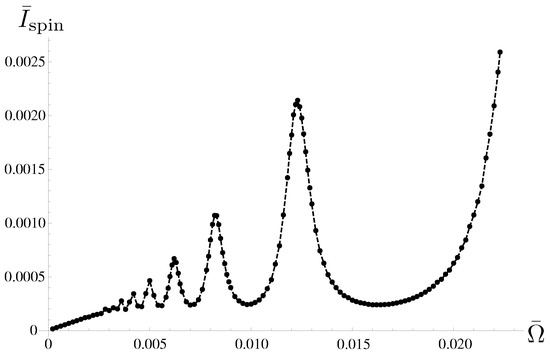
Figure 6. Frequency dependence of the temporal average of spin current $I_{\mathrm{spin}}$. The division number of the step-like precession is now set to $N=20$. With fixed $\delta \varphi =\pi /10$, the frequency is changed by changing $\delta t$. The frequency dependence exhibits two characteristic features: the spin current depends linearly on $\overline{\mathsf{\Omega }}$ for $\overline{\mathsf{\Omega }}\lesssim 0.0025$, whereas it exhibits oscillation with respect to $\overline{\mathsf{\Omega }}$ for $\overline{\mathsf{\Omega }}\gtrsim 0.0025$. The other parameters are the same as in Figure 5.

The frequency dependence of $I_{\mathrm{spin}}$ features two characteristic regimes: a low-frequency regime, where $I_{\mathrm{spin}}$ depends linearly on $\mathsf{\Omega }$ ($\overline{\mathsf{\Omega }}\lesssim 0.0025$) and a high-frequency regime, where $I_{\mathrm{spin}}$ exhibits oscillations with respect to $\mathsf{\Omega }$. These characteristics are explained by comparing the time interval $\delta \overline{t}$ and the relaxation time ${\overline{\tau }}_r$ of the population of dot electrons (${\overline{\tau }}_r\approx 5$ in the present case; see Figure 5A). For lower frequencies, for which $\delta \overline{t}\gg {\overline{\tau }}_r$, the numerator of the time integral of $J_{\mathrm{spin}}(t)$ in Equation (36) becomes constant because the instantaneous spin current has already vanished at a certain $\overline{t}\lesssim \delta \overline{t}$ (see Figure 5A), which results in the linear dependence of $I_{\mathrm{spin}}$ on $\overline{\mathsf{\Omega }}$. As $\overline{\mathsf{\Omega }}$ becomes larger and the time interval satisfies $\delta \overline{t}\lesssim {\overline{\tau }}_r$, the angle $\varphi$ changes during the relaxation process. In this situation, the electron dynamics exhibits two extreme features; when $\delta \overline{t}$ is an integer multiple of the period of the Larmor precession $h/2M$, we have resonance enhancement of the transition between half-filled states $|0,1⟩$ and $|1,0⟩$ by the sudden change of $\varphi$ to exhibit a maximum of $I_{\mathrm{spin}}$, whereas it is anti-resonantly suppressed to exhibit a minimum when $\delta \overline{t}$ is a half-integer multiple of the period [58].

Calculating the spin current for different values of $\theta$, we find that the spin polarization of the spin current exhibits a dependence on $\theta$ in that for $0<\theta <\pi /2$ the spin polarization is antiparallel to the z-axis, whereas for $\pi /2<\theta <\pi$ the spin polarization is parallel to the z-axis. For $\theta =0,\pi /2,\pi$, the spin current vanishes because the spin flip in the quantum dot does not occur for $\theta =0,\pi$ or the two half-filled states in the dot $|1,0⟩$ and $|0,1⟩$ degenerate for $\theta =\pi /4$ (see Equation (29)).

Finally, we note that the averaged spin current $I_{\mathrm{spin}}$ diverges with respect to $\overline{\mathsf{\Omega }}$. The divergence is caused by the accumulation of a nonzero impetus of current $J_{\mathrm{spin}}(t)$ just after the sudden change of $\varphi$ (see Figure 5). In Reference [60], we showed that the nonzero impetus of $J_{\mathrm{spin}}(t)$ is an unphysical effect caused by the Born-Markovian approximation, and the divergence is eliminated by taking into account the non-Markovian effect by keeping the upper bound of the time integration in (10) finite.

5. Discussion and Conclusions

In this paper, we reviewed studies which go beyond the conventional adiabatic approximation for open quantum systems to transfer energy quanta and electron spins with using the full counting statistics, which could provide conditions to show quicker transport. We considered a setup consisting of a two-level system representing an anharmonic junction or a quantum dot and its environment(s) representing a canonical or grand canonical ensemble of the energy quanta and the electron to be transferred. We needed to take into account relaxation phenomena in discussing the transfer. In this case, the adiabatic approximation corresponded to the situation where the relevant system such as the two-level system approaches its stationary state faster than the period of modulation, that is, ${\tau }_r^{-1}\gg \mathsf{\Omega }$ with ${\tau }_r$ the relaxation time of the two-level system and $\mathsf{\Omega }$ the modulation frequency. Because the relaxation time is finite, the condition for which the adiabatic approximation is valid corresponds to the much longer period of the modulation than ${\tau }_r$. This means that we can analyze systematic features including adiabatic as well as nonadiabatic features by changing the ratio of the modulation period and ${\tau }_r$. To clarify the relationship between modulation period and ${\tau }_r$, we discretized the external modulation thereby permitting a systematic analysis of the ratio by changing each interval while retaining the validity of the Born–Markov approximation. For energy quanta pumping, we showed that the nonadiabatic effect contributes a new term to the formula for the pumped quantity under the adiabatic approximation. For spin pumping, we showed that adiabaticity made no contribution but nonadiabaticity is essential. Comparing these features, we showed that the adiabatic contribution can vanish when the stationary state does not depend on the external modulation as for spin pumping. This means that we need to pay attention to the feature of the stationary state in using the adiabatic approximation in describing relaxation phenomena. (We would draw the reader’s attention to the differences in the meaning of nonadiabaticity which has been used in the electron charge pumping by modulation of single gate voltage [61,62].)

With the same setup, the role of nonadiabaticity in pumping phenomena involving energy quanta was discussed more extensively under continuous modulation [63] where the relaxation of the two-level system is treated within the Born–Markovian approximation. In recent work of the present authors on the role of the non-Markovian effect on spin pumping phenomena [60], we found that a nonzero impetus of the dynamics of the pumped quantity under the Born–Markovian approximation shows an unphysical effect, especially for higher modulation frequencies or for the short time regimes. Because the instantaneous impetus contributes strongly under continuous modulation, including the non-Markovian effect would also be necessary in pumping phenomena of energy quanta, especially in evaluating the feature under continuous modulation. This situation remains an open problem. In addition, we described in this work the relaxation process with ordered cumulants of up to second order in the system–environment interaction. An extension to higher orders of cumulants is necessary if we are to discuss relaxation phenomena under strong system–environment interactions. The inclusion of cumulants up to infinite order within the Markovian approximation has been discussed for spin pumping phenomena within the linear response regime using the Green functions [19]. To discuss the non-Markovian effect, it would be necessary to include higher-order cumulants, a topic that remains for a future study.

We can find recent extensions of the treatments with full counting statistics into the strong system-environment coupling for heat transfer [64] and electron pumping [65]. The essential idea to go beyond the weak coupling is to use the similarity (unitary) transformations: the polaron transformation (the reaction coordinate mapping) is used in the former (latter) studies, respectively. As mentioned in the general formalism of FCS, it should be noted that we need careful treatments on the joint probability, Equation (2), when we use the similarity (unitary) transformations on the time evolution operator. The transformation of the projective measurement is also necessary to recover the original joint probability (See Reference [45]). It might be necessary to compare the dynamics of transported quantity with and without the transformation of the projective measurement.

Since the treatment of FCS to discuss the nonadiabatic effects on quantum pumping is general, we can apply it to many other cases: One of the most interesting issues is to study the non-adiabatic treatment on the combined effect caused by multiple external parameters such as in References [66,67,68] where adiabatic transport of charge and/or heat is discussed under time-dependent potential and two reservoirs with biased potentials. We can find other issues to remove the adiabatic approximation in spin pumping via a quantum dot between reservoirs with biased chemical potentials [69] and in the quantum transport and/or quantum pumping under dynamical motion of quantum dot [70] based on the recent developments of experimental techniques on microelectromechanical systems [71]. Further, it would be interesting to discuss the non-adiabatic effect on ac-driven electron systems coupled to multiple reservoirs at finite temperature whose adiabatic treatment is discussed in Reference [72]. We expect that these treatments could provide insights to find new applications, such as the design of nanomachines and understanding of the quantum thermodynamics, as well as quicker transport.

References and Notes

- Pekola, J.P.; Saira, O.-P.; Maisi, V.F.; Kemppinen, A.; Möttönen, M.; Pashkin, Y.A.; Averin, D.V. Single-electron current sources: Toward a refined definition of the ampere. Rev. Mod. Phys. 2013, 85, 1421–1472. [Google Scholar] [CrossRef]
- Žutić, I.; Fabian, J.; Sarma, S.D. Spintronics: Fundamentals and applications. Rev. Mod. Phys. 2004, 76, 323. [Google Scholar] [CrossRef]
- Maekawa, S.; Adachi, H.; Uchida, K.-I.; Ieda, J.I.; Saitoh, E. Spin current: Experimental and theoretical aspects. J. Soc. Phys. Jpn. 2013, 82, 102002. [Google Scholar] [CrossRef]
- Cui, L.; Miao, R.; Jiang, C.; Meyhofer, E.; Reddy, P. Perspective: Thermal and thermoelectric transport in molecular junctions. J. Chem. Phys. 2017, 146, 092201. [Google Scholar] [CrossRef]
- Keller, M.W.; Zimmerman, N.M.; Eichenberge, A.L. Current status of the quantum metrology triangle. Metrologia 2007, 44, 505. [Google Scholar] [CrossRef]
- Thouless, D.J. Quantization of particle transport. Phys. Rev. B 1983, 27, 6083. [Google Scholar] [CrossRef]
- Niu, Q.; Thouless, D.J. Quantised adiabatic charge transport in the presence of substrate disorder and many-body interaction. J. Phys. A Math. Gen. 1984, 17, 2453–2462. [Google Scholar] [CrossRef]
- Altshuler, B.L.; Glazman, L.I. Pumping electrons. Science 1999, 283, 1864–1865. [Google Scholar] [CrossRef]
- Switkes, M.; Marcus, C.M.; Campman, K.; Gossard, A.C. An adiabatic quantum electron pump. Science 1999, 283, 1905–1908. [Google Scholar] [CrossRef] [PubMed]
- Büttiker, M.; Thomas, H.; Prêtre, A. Current partition in multiprobe conductors in the presence of slowly oscillating external potentials. Z. Phys. B Condens. Matter 1994, 94, 133–137. [Google Scholar] [CrossRef]
- Brouwer, P.W. Scattering approach to parametric pumping. Phys. Rev. B 1998, 58, R10135. [Google Scholar] [CrossRef]
- Tserkovnyak, Y.; Brataas, A.; Bauer, G.E.W. Enhanced Gilbert Damping in Thin Ferromagnetic Films. Phys. Rev. Lett. 2002, 88, 117601. [Google Scholar] [CrossRef] [PubMed]
- Tserkovnyak, Y.; Brataas, A.; Bauer, G.E.W. Spin pumping and magnetization dynamics in metallic multilayers. Phys. Rev. B 2002, 66, 224403. [Google Scholar] [CrossRef]
- Mucciolo, E.R.; Chamon, C.; Marcus, C.M. Adiabatic Quantum Pump of Spin-Polarized Current. Phys. Rev. Lett. 2002, 89, 146802. [Google Scholar] [CrossRef] [PubMed]
- Avron, J.E.; Elgart, A.; Graf, G.M.; Sadun, L. Geometry, statistics, and asymptotics of quantum pumps. Phys. Rev. B 2000, 62, R10618. [Google Scholar] [CrossRef]
- Moskalets, M.; Büttiker, M. Floquet scattering theory of quantum pumps. Phys. Rev. B 2010, 66, 205320. [Google Scholar] [CrossRef]
- Moskalets, M. Scattering Matrix Approach to Non-Stationary Quantum Transport; Imperial College Press: London, UK, 2011. [Google Scholar]
- Jauho, A.P.; Wingreen, N.S.; Meir, Y. Time-dependent transport in interacting and noninteracting resonant-tunneling systems. Phys. Rev. B 1994, 50, 5528. [Google Scholar] [CrossRef] [PubMed]
- Wang, B.; Wang, J.; Guo, H. Quantum spin field effect transistor. Phys. Rev. B 2003, 67, 092408. [Google Scholar] [CrossRef]
- Zhang, P.; Xue, Q.K.; Xie, X.C. Spin Current through a Quantum Dot in the Presence of an Oscillating Magnetic Field. Phys. Rev. Lett. 2003, 91, 196602. [Google Scholar] [CrossRef]
- Hattori, K. Kondo effect on adiabatic spin pumping from a quantum dot driven by a rotating magnetic field. Phys. Rev. B 2008, 78, 155321. [Google Scholar] [CrossRef]
- Fransson, J.; Galperin, M. Inelastic scattering and heating in a molecular spin pump. Phys. Rev. B 2010, 81, 075311. [Google Scholar] [CrossRef]
- Chen, K.; Zhang, Z. Spin Pumping in the Presence of Spin-Orbit Coupling. Phys. Rev. Lett. 2015, 114, 126602. [Google Scholar] [CrossRef] [PubMed]
- Tatara, G. Green’s function representation of spin pumping effect. Phys. Rev. B 2016, 94, 224412. [Google Scholar] [CrossRef]
- Tatara, G.; Mizukami, S. Consistent microscopic analysis of spin pumping effects. Phys. Rev. B 2017, 96, 064423. [Google Scholar] [CrossRef]
- Tatara, G. Effective gauge field theory of spintronics. Phys. E Low Dimens. Syst. Nanostruct. 2019, 106, 208–238. [Google Scholar] [CrossRef]
- Sinitsyn, N.A.; Nemenman, I. The Berry phase and the pump flux in stochastic chemical kinetics. Europhys. Lett. 2007, 77, 58001. [Google Scholar] [CrossRef]
- Ren, J.; Hänggi, P.; Li, B. Berry-Phase-Induced Heat Pumping and Its Impact on the Fluctuation Theorem. Phys. Rev. Lett. 2010, 104, 170601. [Google Scholar] [CrossRef]
- Sagawa, T.; Hayakawa, H. Geometrical expression of excess entropy production. Phys. Rev. E 2011, 84, 051110. [Google Scholar] [CrossRef]
- Yuge, T.; Sagawa, T.; Sugita, A.; Hayakawa, H. Geometrical pumping in quantum transport: Quantum master equation approach. Phys. Rev. B 2012, 86, 235308. [Google Scholar] [CrossRef]
- Yuge, T.; Sagawa, T.; Sugita, A.; Hayakawa, H. Geometrical Excess Entropy Production in Nonequilibrium Quantum System. J. Stat. Phys. 2013, 153, 412–441. [Google Scholar] [CrossRef]
- Nakajima, S.; Taguchi, M.; Kubo, T.; Tokura, Y. Interaction effect on adiabatic pump of charge and spin in quantum dot. Phys. Rev. B 2015, 92, 195420. [Google Scholar] [CrossRef]
- Berry, M.V. Quantal phase factors accompanying adiabatic changes. Proc. R. Soc. Lond. Math. Phys. Sci. 1984, 392, 45–57. [Google Scholar] [CrossRef]
- Winkler, N.; Governale, M.; König, J. Theory of spin pumping through an interacting quantum dot tunnel coupled to a ferromagnet with time-dependent magnetization. Phys. Rev. B 2013, 87, 155428. [Google Scholar] [CrossRef]
- Rojek, S.; Governale, M.; König, J. Spin pumping through quantum dots. Phys. Status Solidi B 2013, 251, 1912–1923. [Google Scholar] [CrossRef]
- Jahn, B.O.; Ottosson, H.; Galperin, M.; Fransson, J. Organic Single Molecular Structures for Light Induced Spin-Pump Devices. ACS Nano 2013, 7, 1064–1071. [Google Scholar] [CrossRef] [PubMed]
- Cota, E.; Aguado, R.; Platero, G. ac-Driven Double Quantum Dots as Spin Pumps and Spin Filters. Phys. Rev. Lett. 2005, 94, 107202. [Google Scholar] [CrossRef] [PubMed]
- Braun, M.; Murkard, G. Nonadiabatic Two-Parameter Charge and Spin Pumping in a Quantum Dot. Phys. Rev. Lett. 2008, 101, 036802. [Google Scholar] [CrossRef] [PubMed]
- Cavaliere, F.; Governale, M.; König, J. Nonadiabatic Pumping through Interacting Quantum Dots. Phys. Rev. Lett. 2009, 103, 136801. [Google Scholar] [CrossRef]
- Rojek, S.; König, J.; Shnirman, A. Adiabatic pumping through an interacting quantum dot with spin-orbit coupling. Phys. Rev. B 2013, 87, 075305. [Google Scholar] [CrossRef]
- Splettstoesser, J.; Governale, M.; König, J. Adiabatic charge and spin pumping through quantum dots with ferromagnetic leads. Phys. Rev. B 2008, 77, 195320. [Google Scholar] [CrossRef]
- Riwar, R.; Splettstoesser, J. Charge and spin pumping through a double quantum dot. J. Phys. Rev. B 2010, 82, 205308. [Google Scholar] [CrossRef]
- Esposito, M.; Harbola, U.; Mukamel, S. Entropy fluctuation theorems in driven open systems: Application to electron counting statistics. Phys. Rev. E 2007, 76, 031132. [Google Scholar] [CrossRef] [PubMed]
- Esposito, M.; Harbola, U.; Mukamel, S. Nonequilibrium fluctuations, fluctuation theorems, and counting statistics in quantum systems. Rev. Mod. Phys. 2009, 81, 1665. [Google Scholar] [CrossRef]
- In dealing with a certain open quantum system with a strong system-bath coupling, one may intend to apply a similarity (unitary) transformation, represented by S and S−1, to the total system Hamiltonian. However, in the full counting statistics, it needs a careful treatment. The ultimate goal of the full counting statistics is to calculate a certain statistical quantity provided by the two point measurement described by the joint probability, Equation (2). By application of the similarity transformation, the time evolution operator as well as the projection operators in Equation (2) are transformed as Tr[(Pqti+1S)(S−1U(ti+1,ti)S)(S−1Pqti)W(ti)(PqtiS)(S−1U†(ti+1,ti)S)(S−1Pqti+1)]. This means that we need to pay attention that the projection operator should also be transformed to recover the original joint probability. However, we can avoid the difficulty when the similarity transformation commutes with the projection, [S, Pqt] = 0.
- Kubo, R. Stochastic Liouville Equations. J. Math. Phys. 1963, 4, 174–183. [Google Scholar] [CrossRef]
- Hänggi, P.; Thomas, H. Time evolution, correlations, and linear response of non-Markov processes. Z. Phys. B Condens. Matter 1977, 26, 85–92. [Google Scholar] [CrossRef]
- Hashitsume, N.; Shibata, F.; Shingu, M. Quantal master equation valid for any time scale. J. Stat. Phys. 1977, 17, 155–169. [Google Scholar] [CrossRef]
- Shibata, F.; Takahashi, F.; Hashitsume, N. A generalized stochastic liouville equation. Non-Markovian versus memoryless master equations. J. Stat. Phys. 1977, 17, 171–187. [Google Scholar] [CrossRef]
- Chaturvedi, S.; Shibata, F. Time-convolutionless projection operator formalism for elimination of fast variables. Applications to Brownian motion. Z. Phys. 1979, 35, 297–308. [Google Scholar] [CrossRef]
- Shibata, F.; Arimitsu, T. Expansion Formulas in Nonequilibrium Statistical Mechanics. J. Phys. Soc. Jpn. 1980, 49, 891–897. [Google Scholar] [CrossRef]
- Uchiyama, C.; Shibata, F. Unified projection operator formalism in nonequilibrium statistical mechanics. Phys. Rev. E 1999, 60, 2636. [Google Scholar] [CrossRef]
- Breuer, H.-P.; Petruccione, F. The Theory of Open Quantum Systems; Oxford University Press: New York, NY, USA, 2002. [Google Scholar]
- Segal, D.; Nitzan, A. Heat rectification in molecular junctions. J. Chem. Phys. 2005, 122, 194704. [Google Scholar] [CrossRef] [PubMed]
- Segal, D. Heat flow in nonlinear molecular junctions: Master equation analysis. Phys. Rev. B 2006, 73, 205415. [Google Scholar] [CrossRef]
- Uchiyama, C. Nonadiabatic effect on the quantum heat flux control. Phys. Rev. E 2014, 89, 052108. [Google Scholar] [CrossRef] [PubMed]
- The steplike rotation of the magnetization is experimentally feasible by applying a periodic pulse train of magnetic field on the quantum dot along z-axis. If the magnetic field is strong enough and the pulse interval is sufficiently longer than the Larmor period of the magnetization under the magnetic field, dynamic of the magnetization is well described by the steplike motion.
- Hashimoto, K.; Tatara, G.; Uchiyama, C. Nonadiabaticity in spin pumping under relaxation. Phys. Rev. B 2017, 96, 064439. [Google Scholar] [CrossRef]
- We introduce a unit energy ϵu ≡ 2M, a unit angular frequency ωu ≡ 2M/ℏ, and a unit time tu ≡ 2π/ωu, and normalize energy, angular frequency, inverse temperature and time as ≡ ω/ωu, ≡ ω/ωu, ≡ ϵ/ϵu, ≡ β/βu, and ≡ t/tu, respectively.
- Hashimoto, K.; Tatara, G.; Uchiyama, C. Nonadiabaticity in spin pumping under relaxation. Phys. Rev. B 2019, 99, 205304. [Google Scholar] [CrossRef]
- Kaestner, B.; Kashcheyevs, V. Non-adiabatic quantized charge pumping with tunable-barrier quantum dots: a review of current progress. Rep. Prog. Phys. 2015, 78, 103901. [Google Scholar] [CrossRef] [PubMed]
- Potanina, E.; Brandner, K.; Flindt, C. Optimization of quantized charge pumping using full counting statistics. Phys. Rev. B 2019, 99, 035437. [Google Scholar] [CrossRef]
- Watanabe, K.L.; Hayakawa, H. Non-adiabatic effect in quantum pumping for a spin-boson system. Prog. Theor. Exp. Phys. 2014, 2014, 113A01. [Google Scholar] [CrossRef][Green Version]
- Wang, C.; Ren, J.; Cao, J. Unifying quantum heat transfer in a nonequilibrium spin-boson model with full counting statistics. Phys. Rev. A 2017, 95, 023610. [Google Scholar] [CrossRef]
- Restrepo, S.; Böhling, S.; Cerrillo, J.; Schaller, G. Electron pumping in the strong coupling and non-Markovian regime: A reaction coordinate mapping approach. Phys. Rev. B 2019, 100, 035109. [Google Scholar] [CrossRef]
- Entin-Wohlman, O.; Aharony, A. Adiabatic transport in nanostructures. Phys. Rev. B 2002, 65, 195411. [Google Scholar] [CrossRef]
- Crépieux, A.; Šimkovic, F.; Cambon, B.; Michelini, F. Enhanced thermopower under a time-dependent gate voltage. Phys. Rev. B 2011, 83, 153417. [Google Scholar] [CrossRef]
- Ludovico, M.F.; Battista, F.; von Oppen, F.; Arrachea, L. Adiabatic response and quantum thermoelectrics for ac-driven quantum systems. Phys. Rev. B 2016, 93, 075136. [Google Scholar] [CrossRef]
- Hammar, H.; Jaramillo, J.D.V.; Fransson, J. Spin-dependent heat signatures of single-molecule spin dynamics. Phys. Rev. B 2019, 99, 115416. [Google Scholar] [CrossRef]
- Bode, N.; Kusminskiy, S.V.; Egger, R.; von Oppen, F. Current-induced forces in mesoscopic systems: A scattering-matrix approach. Beilstein J. Nanotechnol. 2012, 3, 144–162. [Google Scholar] [CrossRef] [PubMed]
- Craighead, H.G. Nanoelectromechanical Systems. Dynamics of energy transport and entropy production in ac-driven quantum electron systems. Science 2000, 290, 1532–1535. [Google Scholar] [CrossRef] [PubMed]
- Ludovico, M.F.; Moskalets, M.; Sánchez, D.; Arrachea, L. Dynamics of energy transport and entropy production in ac-driven quantum electron systems. Phys. Rev. B 2016, 94, 035436. [Google Scholar] [CrossRef]
- Haken, H. Synergetics: An Introduction: Nonequilibrium Phase Transitions and Self-Organization in Physics, Chemistry, and Biology; Springer: New York, NY, USA, 1983. [Google Scholar]
© 2019 by the authors. Licensee MDPI, Basel, Switzerland. This article is an open access article distributed under the terms and conditions of the Creative Commons Attribution (CC BY) license (http://creativecommons.org/licenses/by/4.0/).