Abstract
Extending our previous work, quantum dynamic simulations are performed to study low temperature heat transport in a spin-boson model where a two-level subsystem is coupled to two independent harmonic baths. Multilayer multiconfiguration time-dependent Hartree theory is used to numerically evaluate the thermal flux, for which the bath is represented by hundreds to thousands of modes. The simulation results are compared with the approximate Redfield theory approach, and the physics is analyzed versus different physical parameters.
1. Introduction
Electronic and optical processes are usually accompanied by heat generation and transport. Very often, a central task in technology and engineering is to have such transport processes under control. This is particularly useful in the exploration of new nano-size electronic and optical materials, for example, nanoscale molecular junctions where molecules are connected to metal or semiconductor electrodes. Heat transport is crucial for the stability of such junctions, that is, whether the heat generated at such a scale can be released quickly and efficiently is an important characteristic for a potential molecular electronic device [1,2,3,4,5,6]. It has been shown experimentally that the localized Joule heating may induce a substantial temperature increase within a molecule–metal contact due to inefficient heat dissipation [4]. Theoretical modeling and simulation of heat transport at the nanoscale will thus provide valuable insight into the transport mechanisms, as well as offer interpretation of experimental results and help design practical nanoscale electronic devices.
Heat transport through molecular junctions has been modeled by Segal and coworkers [7,8,9] using a system–bath Hamiltonian where a subsystem (representing a junction) is linearly coupled to two heat baths with different temperatures. When the junction is modeled by a harmonic oscillator, the overall problem is trivially solvable. As soon as the junction becomes a two-level system, which can be viewed as a minimal nonlinear model for the junction heat transport, the Hamiltonian becomes the well-known spin-boson model and exhibits rich physics without closed-form solutions. In the weak system–bath coupling regime, Redfield theory [10,11] can be used to provide an approximate description for the heat transport process [7,8,9]. These studies reviewed possible new nano-devices such as a thermal rectifier [7,8], a molecular heat pump [9] and an absorption refrigerator [12,13]. Since charge and heat currents could be coupled, a nonlinear phonon-thermoelectric device was studied [14]. Recently the interference effects in vibrational heat conduction across single-molecule junctions has also been discussed [15].
The weak-coupling assumption in the Redfield theory is, however, often violated in realistic situations. Improved approximations may be developed, e.g., an analog of the Meir–Wingreen formula [16], a nonequilibrium polaron-transformed Redfield equation for bridging the energy transfer from weak to strong coupling regimes [17,18,19,20,21,22], and a full counting statistics combined with the Keldysh nonequilibrium Green’s function, path integral, quantum-classical Liouville equation [23,24,25,26]. These theoretical development offered valuable insights into the heat transport processes.
To gauge the accuracy of these theoretical results it is important to develop numerically exact treatment of the model, which can be used to study stronger coupling regimes and to provide benchmark results for developing approximate theories. In our previous work [27], we have applied the multilayer multiconfiguration time-dependent Hartree (ML-MCTDH) theory [28,29] to study the dynamics of the spin-boson nanojunction model. In contrast to Redfield theory, our previous study revealed a turnover behavior of the heat current with respect to the coupling strength between the two-level system and the heat baths. As a consequence, the optimization of heat transport is possible by choosing an appropriate set of physical parameters. In this work, we extend our simulation to the low temperature regime where quantum effects are more pronounced. Section 2 discusses the model and a few details of implementation of ML-MCTDH for studying heat transport in the spin-boson model. Section 3 presents the results from the ML-MCTDH simulation at low temperature versus several physical parameters. Section 4 concludes.
2. Methods
2.1. Hamiltonian
As in the previous work [7,8,9,16,27] we use a spin-boson type Hamiltonian where two states of the model molecular junction are coupled to two phonon baths, left (L) and right (R). The overall Hamiltonian has three parts
where describes the two-level subsystem
describes the two harmonic baths in mass-weighted coordinates
describes the coupling between the two-level subsystem and the phonon baths
and , are standard Pauli matrices
In this Hamiltonian, the system–bath coupling is off-diagonal in the system states. A simple transformation can be used to convert it to the more familiar spin-boson form [30]. Using the relation
where
and can be transformed to
Thus, is the Hamiltonian used in the simulation.
The system–bath coupling strength parameters ’s are determined by the bath spectral densities [30]
In this model study, we choose identical spectral densities for the left and right bath, which is in an Ohmic form with an exponential cutoff
where is the characteristic frequency of the bath and the Kondo parameter is related to the classical reorganization energy (in the context of electron transfer theories [31] using the spin-boson model) via the relation . In ML-MCTDH simulations the two continuous baths are discretized to a finite number of modes [29], that is, casting the continuous form of Equation (10) to the discrete form in Equation (9). This can be done using several strategies [32,33,34,35] and for a bath with complex glassy spectral densities [33]. The number of bath modes is increased until convergence is achieved, which will be illustrated in the next section.
2.2. Calculating the Heat Current
The heat current or thermal flux is defined as the time derivative of the collective total energy for a heat bath. We can consider an idealized situation that at time zero the two baths are brought into contact with the two-level subsystem. We denote the temperatures as and for the left and right bath, respectively and, without loss of generality, impose the condition that the left bath has a lower temperature, . As time evolves the energy will start to flow among the two baths and the two-level subsystem. The time-dependent energies of the left and right bath can be defined as (we use atomic units where )
where
represents the Hamiltonian for the left and right bath, respectively, and is an initial density matrix of the overall system. The specific choice of affects the transient dynamics of the heat transport, but due to the smallness of the subsystem it does not affect the steady-state heat current. So for convenience, is often chosen in a separable form
where , with the Boltzmann constant, and is an initial density matrix for the two-level subsystem. In this work, we choose to be the identity operator for the two-level subsystem.
The existence of the system–bath coupling makes the definition of the energy for each bath somewhat ambiguous. Here we have used of Equation (12) to define the energy and subsequently the heat current of the left/right bath. On the other hand, the Hamiltonians of the bare baths, of Equation (3), could also be used
For simulation purposes, both definitions give the same long time limit of the steady-state heat current [27], defined as the time-derivative of the bath energy. The use of Equation (12) reduces the magnitude of the transient current and is thus preferred in the simulation. Thereby, the heat current is defined as the energy flux of the left or the right bath (note that we have chosen , so the steady-state energy flow will be from the right to the left)
Based on Equations (1), (7), (8), and (12), the commutators are given as
where is the third Pauli matrix
The short time transient behavior of is different from that of [27]. Their average
generally minimizes the large transient characteristic [27], and will be used to calculate the heat current in our simulation.
The quantum mechanical trace in the the expressions above is evaluated via Monte Carlo average using an importance sampling technique [29,36,37,38]. Unlike some reduced properties such as the system population or a reduced density matrix for a particular degree of freedom, calculating the heat current involves all degrees of freedom for a bath. The statistical average and the finite-mode representation of the bath sometimes may cause to oscillate versus time. This is similar to a quantum reactive scattering calculation in the presence of a scattering continuum where, with a finite number of basis functions, an appropriate absorbing boundary condition is added to mimic the correct outgoing Green’s function [39,40,41,42]. In a previous work [27], we employed such a strategy to regularize the heat current at longer time
where the regularization parameter resembles the formal convergence parameter in the definition of the Green’s function in terms of the time evolution operator
and is chosen in a similar way as the absorbing potential used in quantum scattering calculations [39,40,41,42]: large enough to accelerate the convergence but still sufficiently small in order not to affect the correct result. This regularization scheme was used in our previous work [27] to mainly compensate for the finite-mode representation of the bath. In this work, however, the numbers of bath modes are sufficiently large to render this effect unimportant. On the other hand, we found oscillations in due to the Monte Carlo integration of an oscillatory integrand, which is indicated from the observation that the amplitude of the oscillations decreases roughly versus the inverse of the square root of the statistical samples/initial wave functions. We could average out such oscillations by significantly increasing the numbers of samples, which would be too expensive. Instead, we have used time averaging, which is an effective approach for reducing such oscillations in . Thereby, the time-averaged is defined as
where is the cutoff time when the time averaging starts. We found this approach simpler to implement and it allows us to achieve convergence with a reasonable number of statistical samples. The performance will be discussed in the result section.
2.3. Multilayer Multiconfiguration Time-Dependent Hartree Theory
The simulation of the heat current in Equations (15)–(18) involves the evaluation of a quantum mechanical trace and real time propagation for each wave function. The quantum mechanical trace for evaluating the physical observables has the general form
In case that the initial density matrix can be diagonalized, i.e.,
Equation (22) reduces to a simple summation
which can be carried out by Monte Carlo importance sampling methods [29,36,37,38]. On the other hand, when cannot be trivially diagonalized, more sophisticated methods are available to cast Equation (22) into a sum of wave functions with proper weight [37,38]. In this work, each result is obtained from averaging over a few hundred to a few thousand samples/wave functions.
The time evolution for each wave function of the sample, , is achieved by employing the multilayer multiconfiguration time-dependent Hartree (ML-MCTDH) theory [29]. ML-MCTDH is a variational method to propagate a wave function of a large system with many degrees of freedom. In this approach a recursive, layered expansion is used to represent a wave function
where , , and so on are the expansion coefficients for the first, second, third,..., layers, respectively; , , ,..., are the single particle functions (SPFs) for the first, second, third,..., layers. The multilayer hierarchy terminates at the bottom level by expressing the SPFs in this layer in terms of (contracted) primitive basis functions. The variational parameters within the ML-MCTDH framework are dynamically optimized through the use of Dirac–Frenkel variational principle [43]
which results in a set of coupled, nonlinear differential equations [28,29,44,45,46]. The equations of motion can be effectively propagated using a singular value decomposition (SVD)-based algorithm [47,48]. The ML-MCTDH theory has been generalized to treat identical particles explicitly by employing the second quantized representation [49]. A review of this topic can be found in a recent publication [50]. Furthermore, ML-MCTDH can also be used for calculating energy eigenstates [34,35] or equilibrium reduced density matrices [51].
The form of the ML-MCTDH wave function in Equation (25) has also received much attention recently in applied mathematics [52,53,54]. The original single-layer MCTDH [55,56,57,58] obeys the so-called Tucker form [59] of tensor decomposition. ML-MCTDH [28,29] is then naturally called the hierarchical Tucker (H-Tucker) form and is in fact acknowledged as the first occurrence of the H-Tucker tensor format [52,53,54]. Sometimes it is also called the tree tensor network, although this term or the H-Tucker format usually refers to a binary tree branching structure [53]. Most times a balanced tree is constructed for an ML-MCTDH wave function. For a binary-splitting tree, an layer representation holds bottom layer SP groups (in our accounting the root node wave function does not count as a layer, the first layer comes from the next level). There is also a special skewed tree structure called the tensor train format in mathematics and the matrix-product states in physics [54].
In this work, we adopted a semi-binary tree structure. There are three SP nodes in the first layer, one for the two-level system, one for the left bath, and another one for the right bath. The tree node for the two-level group terminates at the first layer, whereas each node for the left- and right-bath generates two nodes at the next level (the second layer). This binary branching continues until all the bath degrees freedom can be included in the bottom layer. We have used mode combination and basis function contraction [36], under which each bottom-layer SP group may hold up to five bath degrees of freedom. As a result, we have used 6–10 layers in this work to study heat transport where each bath is discretized by a few hundred to a thousand modes. The choice of this semi-binary tree is for convenience and is due to the simplicity of the bath spectral density. For a model with many intramolecular modes, a more complex tree structure may be used [60].
3. Results and Discussion
In this work, we focus on studying heat transport dynamics of the spin-boson model at low temperatures: the left bath has zero temperature whereas the temperature of the right bath is a physical parameter. Other physical parameters include the reorganization energy and the characteristic frequency in Equation (10), chosen to be the same for the two baths, as well as the energy spacing in Equation (7) for the two-level system. The relative error for the simulations were controlled to be less than based on estimates from repeated ML-MCTDH convergence tests by varying the numbers of primitive basis functions, SPFs, bath degrees of freedom, and statistical samples. Some of these are discussed below. In a typical production run, a total of 1000–2000 bath (left + right) modes were required. This number is greater than that used in the previous work [27], primarily due to the low temperatures. This is because a large density of states is needed to model the condensed phase environment within a finite time of simulation. At lower temperature this translates to more modes. For all the bath modes the number of primitive basis functions ranges from three (for high-frequency modes) to a few tens (for low-frequency modes). A total of 6–10 layers were used in ML-MCTDH simulations. Overall, it appears that the statistical uncertainty is the bottleneck of the calculational error.
Figure 1 shows the convergence of the time-dependent heat current versus two set of simulation parameters, different configuration space settings and different numbers of the bath modes. The physical parameters are as follows: the reorganization energy cm and the characteristic frequency cm (the same for the two baths), the system energy spacing cm, and the temperatures are and K. Figure 1a shows a typical variation of versus configuration settings when the configuration space is large enough. As mentioned earlier, we adopted a semi-binary tree structure. There are three SP nodes at the first layer, one for the two-level system, one for the left bath, and another one for the right bath. Each tree node for the left- and right-bath generates two nodes at the next level and so on until all the bath degrees freedom can be included in the bottom layer. In this case, there are 500 modes for each bath, and seven layers are used in the simulation. The results are within a few percent of each other, so any setting will do. For most of the results shown in this paper, we used settings similar to configuration C, that is, 16 SPFs (256 configurations under the link node) for the top half number of layers, and 8 SPFs (64 configurations under the link node) for the bottom half layers. It should be noted that although the steady state (averaged) current is converged to within a few percent, this configuration set may not be sufficient for some other purposes. For example, it does not produce a perfect plateau, but a line with a small slope. Using a larger configuration set removes this artifact but at a considerably high cost.
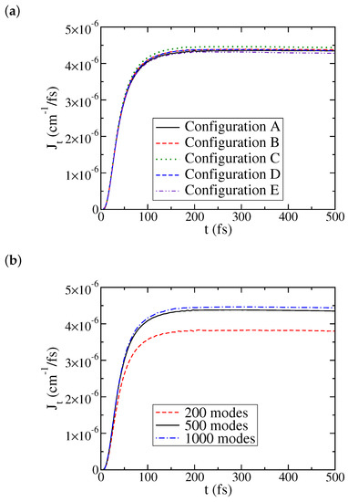
Figure 1.
Convergence of for the set of physical parameters: cm, cm, cm, , K, and versus: (a) different configuration settings with 500 modes for each bath, where Configuration A: and (meaning 20 single particle functions (SPFs) for each SP group of the top four layers, and 10 SPFs for each SP group of the bottom three layers); Configuration B: and ; Configuration C: and ; Configuration D: and ; Configuration E: and ; and (b) different numbers of bath modes for each bath.
Figure 1b shows the necessity of using a sufficient number of bath modes to obtain accurate heat current. With 200 modes for each bath, both the transient and the steady-state currents have relatively large deviations from the converged results. For results discussed in this paper, we used 500–1000 modes for each bath. The resulting error in is estimated to be a few percent.
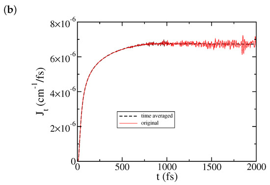
Next we show the effect of time averaging in Equation (21) on . Figure 2a illustrates for the same set of physical parameters as in Figure 1 where 1000 modes were used for each bath in the simulation. The steady-state plateau for the heat current is established in a relatively short time, so the time averaging can start relatively early, any time between 200 and 500 fs (here we use fs) in Equation (21). As shown in Figure 2a, the time-averaged removes the small oscillations at longer time, and gives a more stable value of the steady-state heat current. In this case, time averaging was not really necessary if one is only interested in the steady-state current already established earlier. On the other hand, Figure 2b illustrates a situation where establishes a plateau in a much later time. In this case, longer time propagation was needed with displaying larger amplitude oscillations. The starting time for time averaging is later, at fs in Equation (21). Figure 2b shows that time averaging works quite well for providing a sensible steady-state current. Thus, for the results discussed below the time-averaged will be used.

We now discuss the dependence of the heat current on some physical parameters. Figure 3 illustrates the dynamics of with respect to two parameters, the characteristic frequency of the bath and the system–bath coupling strength (the bath reorganization energy), chosen to be the same for the left and the right bath. The remaining physical parameters are the same as in Figure 1, and 1000 modes are used to represent each bath. The dependence on the bath characteristic frequency is quite pronounced. As shown in Figure 3a, the steady state current decreases as decreases, and almost diminishes at cm. While our result reveals that a transport blockade occurs at cm for this set of physical parameters, it does not mean that along the opposite direction the heat current keeps increasing with respect to characteristic frequency . Instead, for a larger , does not reach a well-defined plateau within a simulation time of 4 ps, suggesting long transient coherent behavior.
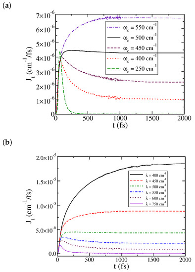
Figure 3.
Dependence of on: (a) the characteristic frequency of the bath, and (b) the reorganization energy of the bath, . The remaining physical parameters are the same as in Figure 1.
In a previous study [27], we have found a turnover behavior of the heat current with respect to the system–bath coupling strength that resembles the Kramers turnover for the rate constant [61,62]. As shown in Figure 3b, this turnover behavior does not show up with the current set of parameters and at low temperatures. A similar observation has been made for the rate constants at low temperatures [37]. Figure 3b shows the ML-MCTDH simulated steady-state heat current monotonically decreases when the coupling strength increases, and is essentially blocked as the coupling reaches a certain level. Again, this does not mean that along another direction the heat current continuously increases as decreases. For a small , exhibits long transient coherent behavior and does not reach a well-defined plateau within the simulation time.
Figure 4 illustrates the dynamics of versus the energy spacing of the two-level system . The remaining physical parameters are the same as in Figure 1, and 1000 modes are used to represent each bath. This dependence on is what one would expect from a Fermi golden rule approximation treating as the perturbation parameter, i.e., , but not from the Redfield theory where the system–bath coupling is the perturbation parameter. Given the value of cm , it is reasonable to assume that the golden rule approach is more appropriate.
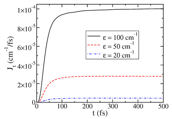
Figure 4.
Dependence of on the the energy spacing of the two-level system . The remaining physical parameters are the same as in Figure 1.
The last physical parameter is illustrated in Figure 5, which shows the dependence of the steady-state heat current J on the temperature of the right bath, , while the left bath is at zero temperature and the remaining physical parameters are the same as in Figure 1. As expected, the heat current increases as increases.
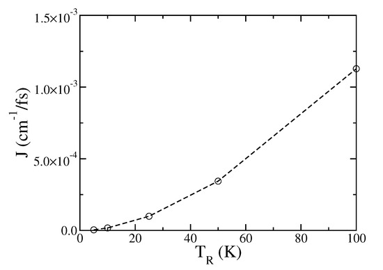
Figure 5.
Dependence of the steady-state heat current J on the temperature of the right bath, . The remaining physical parameters are the same as in Figure 1. The line serves as a guide to the eye.
One may be curious about the performance of Redfield theory that was initially used in the study of heat transport in the spin-boson model [7,8,9,16,27]. The following discussions compare the Redfield approximation with our ML-MCTDH simulations. First shown in Figure 6 is the dependence of the heat current on the characteristic frequency. Not only are the Redfield currents much bigger than our simulation results, but also the trend is different: while our ML-MCTDH simulation predicts an increase in the heat current as the characteristic frequency increases, Redfield theory predicts the opposite—that J decreases upon increasing . The disagreement can be rationalized by noting the value of the system–bath coupling, cm, which is not in the weak coupling regime that Redfield theory operates. In addition, the steady-state Redfield theory used here [7,8,9] assumes that heat transfer is dominated by resonance energy transmission and that dephasing processes are fast, neither is satisfied for the set of physical parameters in the low-temperature heat transport processes studied here.
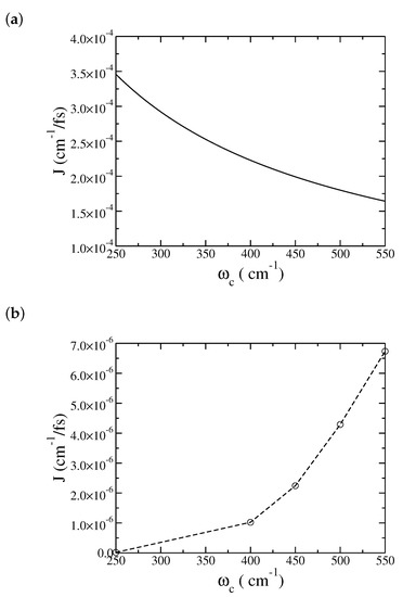
Figure 6.
Dependence of the steady-state heat current J on the characteristic frequency of the bath : (a) Redfield results, and (b) multilayer multiconfiguration time-dependent Hartree (ML-MCTDH) results. The remaining physical parameters are the same as in Figure 1.
Figure 7 shows both Redfield approximation (Figure 7a) and our ML-MCTDH simulations (Figure 7b) where the system–bath coupling is varied. Again, Redfield theory gives too large current values, and also an opposite trend for J versus in comparison with the simulation results. As discussed in a previous work [16], Redfield theory is no long a good approximation as the system–bath coupling increases. A turnover behavior of the heat current with respect to the system–bath coupling strength will be observed [27] and is best described by some improved theories [16,17,22]. On the other hand, Figure 7b does not show a turnover behavior at low temperatures. As discussed earlier, this is because the steady-state current is not well defined (at low temperatures) for a weak system–bath coupling , where exhibits long time coherent behavior instead of reaching a well-defined plateau. In this weak coupling regime, it is an interesting future task to study transient dynamics and possibly how to use this information to extract the steady-state current at very long time.
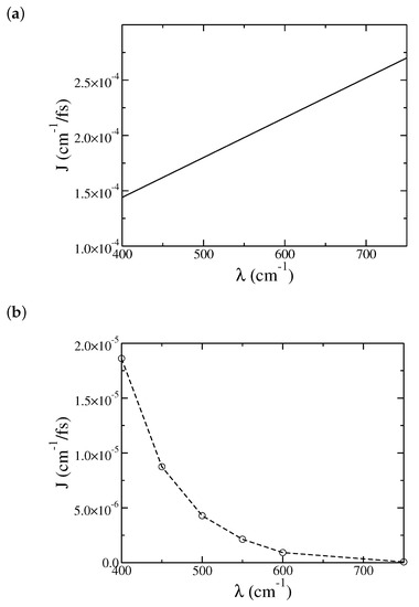
Figure 7.
Dependence of the steady-state heat current J on the reorganization energies of the bath, : (a) Redfield results, and (b) ML-MCTDH results. The remaining physical parameters are the same as in Figure 1.
For most of the parameter sets considered in the paper, the ML-MCTDH simulated heat currents are almost two orders of magnitude smaller than the Redfield theory results. Thus, the comparisons were made in separate plots in Figure 6 and Figure 7. Our final comparisons between Redfield theory and the ML-MCTDH simulations are illustrated in Figure 8, in which the results are overlaid. Figure 8a shows the dependence of the steady-state current J on the level spacing of the two-level system. Redfield theory shows a quick drop in the current as increases, which is a manifestation of low temperatures in the Redfield expression. On the other hand, the ML-MCTDH simulation shows an approximate quadratic increase for the heat current as increases, , consistent with the golden rule approximation where is the perturbation parameter. This behavior will eventually breakdown when becomes too large, and will be an interesting subject for the future. Finally, Figure 8b shows the temperature dependence of the steady-state current. In this case, Redfield theory predicts the correct qualitative trend, that J increases as T increases. Its values are, however, too big as compared with the simulation results.
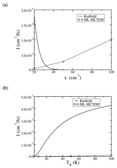
Figure 8.
Dependence of the steady-state heat current J on (a) the energy spacing of the two-level system and (b) the temperature of the right bath, . The solid line is from Redfield theory and the dashed line with circle is from ML-MCTDH simulation (the dashed line serves as a guide to the eye). The remaining physical parameters are the same as in Figure 1.
4. Conclusions
In this paper, we have employed the ML-MCTDH theory to simulate heat transport processes in a spin-boson junction model at low temperatures. Compared with our previous work [27], more bath modes are needed to represent the continuum at low temperatures, thus requiring more layers for the tensor contraction in ML-MCTDH. Time averaging is also a useful technique for obtaining the steady-state current. Dependence of the heat current has been investigated versus several physical parameters, i.e., the energy spacing for the two-level system, the characteristic frequency of the bath, the system–bath coupling strength, and the temperature difference between the two baths. Comparisons have also been made with the Redfield theory approximation. Interesting behavior at low temperature has been observed, primarily of strong quantum origin.
The ML-MCTDH benchmark results will be helpful for developing physical theories to study heat transport processes at low temperatures. This is of both theoretical interest and practical use for designing small devices under extreme conditions. A particularly interesting question, which is beyond this work but worth studying in the future, is whether a steady-state heat transport can ever be established at low temperatures. Under such conditions, the quantum coherence effect may be prominent. Even a steady-state current can be reached at infinite time in theory, finite-time transient dynamics of may be dominant for determining practical heat transport.
Author Contributions
Conceptualization, C.-H.Y. and H.W.; methodology, C.-H.Y. and H.W.; software, C.-H.Y. and H.W.; validation, C.-H.Y. and H.W.; formal analysis, C.-H.Y. and H.W.; investigation, C.-H.Y. and H.W.; resources, H.W.; data curation, C.-H.Y. and H.W.; writing–original draft preparation, C.-H.Y. and H.W.; writing–review and editing, C.-H.Y. and H.W.; visualization, C.-H.Y. and H.W.; supervision, H.W.; project administration, H.W.; funding acquisition, H.W. All authors have read and agreed to the published version of the manuscript.
Funding
This research was funded by the National Science Foundation (NSF) CHE-1954639. This work used the Extreme Science and Engineering Discovery Environment (XSEDE), which is supported by NSF grant number ACI-1548562, and resources of the National Energy Research Scientific Computing Center (NERSC), which is supported by the Office of Science of the U.S. Department of Energy under Contract No. DE-AC02-05CH11231.
Conflicts of Interest
The authors declare no conflict of interest. The funders had no role in the design of the study; in the collection, analyses, or interpretation of data; in the writing of the manuscript, or in the decision to publish the results.
References
- Montgomery, M.J.; Todorov, T.N.; Sutton, A.P. Power dissipation in nanoscale conductors. J. Phys. Condens. Matter 2002, 14, 5377. [Google Scholar] [CrossRef]
- Chen, Y.C.; Zwolak, M.; Ventra, M.D. Local Heating in Nanoscale Conductors. Nano Lett. 2003, 3, 1691. [Google Scholar] [CrossRef]
- Segal, D.; Nitzan, A.; Hänggi, P. Thermal conductance through molecular wires. J. Chem. Phys. 2003, 119, 6840. [Google Scholar] [CrossRef]
- Huang, Z.F.; Xu, B.Q.; Chen, Y.C.; Ventra, M.D.; Tao, N.J. Measurement of Current-Induced Local Heating in a Single Molecule Junction. Nano Lett. 2006, 6, 1240. [Google Scholar] [CrossRef]
- Pecchia, A.; Romano, G.; Carlo, A.D. Theory of heat dissipation in molecular electronics. Phys. Rev. B 2007, 75, 035401. [Google Scholar] [CrossRef]
- Ioffe, Z.; Shamai, T.; Ophir, A.; Noy, G.; Yutsis, I.; Kfir, K.; Chesnovsky, O.; Selzer, Y. Detection of heating in current-carrying molecular junctions by Raman scattering. Nat. Nanotechnol. 2008, 3, 727. [Google Scholar] [CrossRef] [PubMed]
- Segal, D.; Nitzan, A. Spin-boson thermal rectifier. Phys. Rev. Lett. 2005, 94, 034301. [Google Scholar] [CrossRef]
- Segal, D.; Nitzan, A. Heat rectification in molecular junctions. J. Chem. Phys. 2005, 122, 194704. [Google Scholar] [CrossRef] [PubMed]
- Segal, D.; Nitzan, A. Molecular heat pump. Phys. Rev. E 2006, 73, 026109. [Google Scholar] [CrossRef] [PubMed]
- Redfield, A.G. On the Theory of Relaxation Processes. IBM J. 1957, 1, 19. [Google Scholar] [CrossRef]
- Redfield, A.G. The Theory of Relaxation Processes. Adv. Magn. Reson. 1965, 1, 1. [Google Scholar]
- Segal, D. Current fluctuations in quantum absorption refrigerators. Phys. Rev. E 2018, 97, 052145. [Google Scholar] [CrossRef] [PubMed]
- Friedman, H.M.; Agarwalla, B.K.; Segal, D. Quantum energy exchange and refrigeration: A full-counting statistics approach. New J. Phys. 2018, 20, 083026. [Google Scholar] [CrossRef]
- Jiang, J.H.; Kulkarni, M.; Segal, D.; Imry, Y. Phonon thermoelectric transistors and rectifiers. Phys. Rev. B 2015, 92, 045309. [Google Scholar] [CrossRef]
- Chen, R.; Sharony, I.; Nitzan, A. Local Atomic Heat Currents and Classical Interference in Single-Molecule Heat Conduction. J. Phys. Chem. Lett. 2020, 11, 4261–4268. [Google Scholar] [CrossRef] [PubMed]
- Velizhanin, K.A.; Thoss, M.; Wang, H. Meir-Wingreen formula for heat transport in a spin-boson nanojunction model. J. Chem. Phys. 2010, 133, 084503. [Google Scholar] [CrossRef]
- Wang, C.; Ren, J.; Cao, J. Nonequilibrium Energy Transfer at Nanoscale: A Unified Theory from Weak to Strong Coupling. Sci. Rep. 2015, 5, 11787. [Google Scholar] [CrossRef]
- Xu, D.; Cao, J. Non-canonical distribution and non-equilibrium transport beyond weak system-bath coupling regime: A polaron transformation approach. Front. Phys. 2016, 11, 110308. [Google Scholar] [CrossRef]
- Wang, C.; Ren, J.; Cao, J. Unifying quantum heat transfer in a nonequilibrium spin-boson model with full counting statistics. Phys. Rev. A 2017, 95, 023610. [Google Scholar] [CrossRef]
- Liu, J.; Hsieh, C.Y.; Wu, C.; Cao, J. Frequency-dependent current noise in quantum heat transfer: A unified polaron calculation. J. Chem. Phys. 2018, 148, 234104. [Google Scholar] [CrossRef]
- Duan, C.; Hsieh, C.Y.; Liu, J.; Wu, J.; Cao, J. Unusual Transport Properties with Noncommutative System–Bath Coupling Operators. J. Phys. Chem. Lett. 2020, 11, 4080–4085. [Google Scholar] [PubMed]
- Hsieh, C.; Liu, J.; Duan, C.; Cao, J. A Nonequilibrium Variational Polaron Theory to Study Quantum Heat Transport. J. Phys. Chem. C 2019, 123, 17196–17204. [Google Scholar]
- Agarwalla, B.K.; Segal, D. Energy current and its statistics in the nonequilibrium spin-boson model: Majorana fermion representation. New J. Phys. 2017, 19, 043030. [Google Scholar]
- Liu, J.; Hsieh, C.Y.; Segal, D.; Hanna, G. Heat transfer statistics in mixed quantum-classical systems. J. Chem. Phys. 2018, 149, 224104. [Google Scholar] [PubMed]
- Kilgour, M.; Agarwalla, B.K.; Segal, D. Path-integral methodology and simulations of quantum thermal transport: Full counting statistics approach. J. Chem. Phys. 2019, 150, 084111. [Google Scholar] [PubMed]
- Liu, H.; Wang, C.; Wang, L.Q.; Ren, J. Strong system-bath coupling induces negative differential thermal conductance and heat amplification in nonequilibrium two-qubit systems. Phys. Rev. E 2019, 99, 032114. [Google Scholar] [PubMed]
- Velizhanin, K.A.; Wang, H.; Thoss, M. Heat transport through model molecular junctions: A multilayer multiconfiguration time-dependent Hartree approach. Chem. Phys. Lett. 2008, 460, 325. [Google Scholar]
- Wang, H.; Thoss, M. Multilayer formulation of the multiconfiguration time-dependent Hartree theory. J. Chem. Phys. 2003, 119, 1289. [Google Scholar]
- Wang, H. Multilayer Multiconfiguration Time-Dependent Hartree Theory. J. Phys. Chem. A 2015, 119, 7951. [Google Scholar]
- Leggett, A.J.; Chakravarty, S.; Dorsey, A.T.; Fisher, M.P.A.; Garg, A.; Zwerger, W. Dynamics of the dissipative two-state system. Rev. Mod. Phys. 1987, 59, 1. [Google Scholar]
- Marcus, R.A. Electron transfer reactions in chemistry. Theory and experiment. Rev. Mod. Phys. 1993, 65, 599. [Google Scholar]
- Wang, H.; Shao, S. Dynamics of a two-level system coupled to a bath of spins. J. Chem. Phys. 2012, 137, 22A504. [Google Scholar] [CrossRef] [PubMed]
- Zhou, Y.; Shao, J.; Wang, H. Dynamics of electron transfer in complex glassy environment modeled by the Cole-Davidson spectral density. Mol. Phys. 2012, 110, 581. [Google Scholar] [CrossRef]
- Wang, H. Iterative Calculation of Energy Eigenstates Employing the Multilayer Multiconfiguration Time-Dependent Hartree Theory. J. Phys. Chem. A 2014, 117, 9253. [Google Scholar] [CrossRef] [PubMed]
- Wang, H.; Shao, J. Quantum Phase Transition in the Spin-Boson Model: A Multilayer Multiconfiguration Time-Dependent Hartree Study. J. Phys. Chem. A 2019, 123, 1882. [Google Scholar] [PubMed]
- Wang, H. Basis set approach to the quantum dissipative dynamics: Application of the multiconfiguration time-dependent Hartree method to the spin-boson problem. J. Chem. Phys. 2000, 113, 9948. [Google Scholar]
- Wang, H.; Skinner, D.E.; Thoss, M. Calculation of reactive flux correlation functions for systems in a condensed phase environment: A multilayer multi-configuration time-dependent Hartree approach. J. Chem. Phys. 2006, 125, 174502. [Google Scholar]
- Wang, H.; Thoss, M. Quantum mechanical evaluation of the Boltzmann operator in correlation functions for large molecular systems: A multilayer multi-configuration time-dependent Hartree approach. J. Chem. Phys. 2006, 124, 034114. [Google Scholar] [CrossRef]
- Goldberg, A.; Shore, B.W. Modelling laser ionisation. J. Phys. B 1978, 11, 3339. [Google Scholar]
- Kosloff, R.; Kosloff, D. Absorbing boundaries for wave propagation problems. J. Comp. Phys. 1986, 63, 363. [Google Scholar] [CrossRef]
- Neuhauser, D.; Baer, M. The application of wave packets to reactive atom-diatom systems: A new approach. J. Chem. Phys. 1989, 91, 4651. [Google Scholar] [CrossRef]
- Seideman, T.; Miller, W.H. Calculation of the cumulative reaction probability via a discrete variable representation with absorbing boundary conditions. J. Chem. Phys. 1992, 96, 4412. [Google Scholar]
- Frenkel, J. Wave Mechanics; Clarendon Press: Oxford, UK, 1934. [Google Scholar]
- Manthe, U. A multilayer multiconfigurational time-dependent Hartree approach for quantum dynamics on general potential energy surfaces. J. Chem. Phys. 2008, 128, 164116. [Google Scholar] [CrossRef]
- Manthe, U. Layered discrete variable representations and their application within the multiconfigurational time-dependent Hartree approach. J. Chem. Phys. 2009, 130, 054109. [Google Scholar] [CrossRef]
- Vendrell, O.; Meyer, H.D. Multilayer multiconfiguration time-dependent Hartree method: Implementation and applications to a Henon-Heiles Hamiltonian and to pyrazine the description of polyatomic molecules. J. Chem. Phys. 2011, 134, 044135. [Google Scholar] [PubMed]
- Wang, H.; Meyer, H.D. On regularizing the MCTDH equations of motion. J. Chem. Phys. 2018, 148, 124105. [Google Scholar]
- Wang, H.; Meyer, H.D. On regularizing the ML-MCTDH equations of motion. J. Chem. Phys. 2019, 149, 044119. [Google Scholar]
- Wang, H.; Thoss, M. Numerically exact quantum dynamics for indistinguishable particles: The multilayer multiconfiguration time-dependent Hartree theory in second quantization representation. J. Chem. Phys. 2009, 131, 024114. [Google Scholar] [CrossRef]
- Lode, A.U.J.; Lévêque, C.; Madsen, L.B.; Streltsov, A.I.; Alon, O.E. Colloquium: Multiconfigurational time-dependent Hartree approaches for indistinguishable particles. Rev. Mod. Phys. 2020, 92, 011001. [Google Scholar]
- Wang, H.; Liu, X.; Liu, J. Accurate calculation of equilibrium reduced density matrix for the system-bath model: A multilayer multiconfiguration time-dependent Hartree approach and its comparison to a multi-electronic-state path integral molecular dynamics approach. Chin. J. Chem. Phys. 2018, 31, 446. [Google Scholar]
- Grasedyck, L. Hierarchical singular value decomposition of tensors. SIAM J. Matrix Anal. Appl. 2010, 31, 2029. [Google Scholar] [CrossRef]
- Grasedyck, L.; Kressner, D.; Tobler, C. A literature survey of low--rank tensor approximation techniques. GAMM-Mitteilungen 2013, 36, 53. [Google Scholar]
- Lubich, C.; Rohwedder, T.; Schneider, R.; Vandereycken, B. Dynamical Approximation by Hierarchical Tucker and Tensor-Train Tensors. SIAM J. Matrix Anal. Appl. 2013, 34, 470. [Google Scholar] [CrossRef]
- Meyer, H.D.; Manthe, U.; Cederbaum, L.S. The multi-configurational time-dependent Hartree approach. Chem. Phys. Lett. 1990, 165, 73. [Google Scholar]
- Manthe, U.; Meyer, H.D.; Cederbaum, L.S. Wave-Packet Dynamics within the Multiconfiguration Hartree Framework: General Aspects and application to NOCl. J. Chem. Phys. 1992, 97, 3199. [Google Scholar] [CrossRef]
- Beck, M.H.; Jäckle, A.; Worth, G.A.; Meyer, H.D. The multiconfiguration time-dependent Hartree (MCTDH) method: A highly efficient algorithm for propagating wavepackets. Phys. Rep. 2000, 324, 1. [Google Scholar]
- Meyer, H.D.; Worth, G.A. Quantum molecular dynamics: Propagating wavepackets and density operators using the multiconfiguration time-dependent Hartree (MCTDH) method. Theor. Chem. Acc. 2003, 109, 251. [Google Scholar]
- Tucker, L.R. Some mathematical notes of three-mode factor analysis. Psychometrika 1966, 31, 279. [Google Scholar] [CrossRef]
- Yang, C.H.; Denne, J.; Reed, S.; Wang, H. Computational study on the removal of photolabile protecting groups by photochemical reactions. Comput. Theor. Chem. 2019, 1151, 1. [Google Scholar]
- Pollak, E. Theory of activated rate processes: A new derivation of Kramers expression. J. Chem. Phys. 1986, 85, 865. [Google Scholar]
- Hänggi, P.; Talkner, P.; Borkovec, M. Reaction-rate theory: Fifty years after Kramers. Rev. Mod. Phys. 1990, 62, 251. [Google Scholar] [CrossRef]


© 2020 by the authors. Licensee MDPI, Basel, Switzerland. This article is an open access article distributed under the terms and conditions of the Creative Commons Attribution (CC BY) license (http://creativecommons.org/licenses/by/4.0/).