Figure 1.
The flow chart of CPE algorithm. The left part of this flow chart is the basic steps, and the right is the key steps of CPE algorithm called the secondary partitioning which aims to obtain the coded sequence matrix .
Figure 1.
The flow chart of CPE algorithm. The left part of this flow chart is the basic steps, and the right is the key steps of CPE algorithm called the secondary partitioning which aims to obtain the coded sequence matrix .
Figure 2.
The processes of calculating PE and CPE for a simple example. For the secondary partitioning in CPE, using the serial number constructs as shown in the bold red line, and records the size of the relationship between and as the bold blue line shown.
Figure 2.
The processes of calculating PE and CPE for a simple example. For the secondary partitioning in CPE, using the serial number constructs as shown in the bold red line, and records the size of the relationship between and as the bold blue line shown.
Figure 3.
Synthetic signal .
Figure 3.
Synthetic signal .
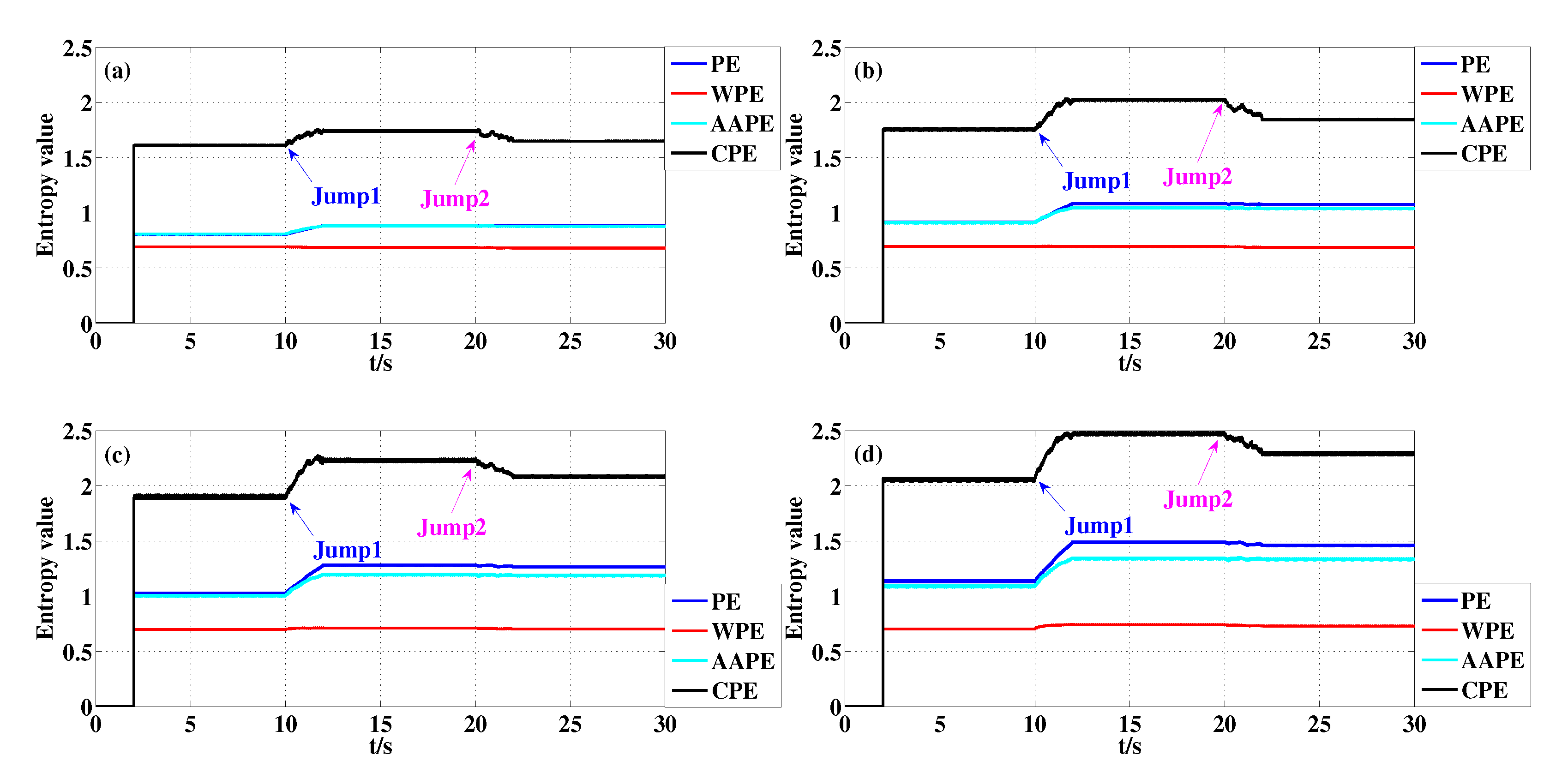
Figure 4.
Detecting dynamical changes existing in the synthetic signal with different m using PE, WPE, AAPE, and CPE: (a) ; (b) ; (c) ; (d) .
Figure 4.
Detecting dynamical changes existing in the synthetic signal with different m using PE, WPE, AAPE, and CPE: (a) ; (b) ; (c) ; (d) .
Figure 5.
The transient logistic map.
Figure 5.
The transient logistic map.
Figure 6.
Detecting dynamical changes existing in the transient logistic map with different m using PE, WPE, AAPE, and CPE: (a) ; (b) ; (c) ; (d) .
Figure 6.
Detecting dynamical changes existing in the transient logistic map with different m using PE, WPE, AAPE, and CPE: (a) ; (b) ; (c) ; (d) .
Figure 7.
The transient Lorenz map.
Figure 7.
The transient Lorenz map.
Figure 8.
Detecting dynamical changes existing in the transient Lorenz map with different m using PE, WPE, AAPE, and CPE: (a) ; (b) ; (c) ; (d) .
Figure 8.
Detecting dynamical changes existing in the transient Lorenz map with different m using PE, WPE, AAPE, and CPE: (a) ; (b) ; (c) ; (d) .
Figure 9.
The performance of four algorithms in distinguishing periodic series and chaotic series under different SNR when : (a) PE; (b) WPE; (c) AAPE; (d) CPE.
Figure 9.
The performance of four algorithms in distinguishing periodic series and chaotic series under different SNR when : (a) PE; (b) WPE; (c) AAPE; (d) CPE.
Figure 10.
Detecting abnormal pulse existing in IRF signal with different m using PE, WPE, AAPE, and CPE: (a) The IRF signal; (b) ; (c) ; (d) .
Figure 10.
Detecting abnormal pulse existing in IRF signal with different m using PE, WPE, AAPE, and CPE: (a) The IRF signal; (b) ; (c) ; (d) .
Figure 11.
Detecting abnormal pulse existing in BF signal with different m using PE, WPE, AAPE, and CPE: (a) The BF signal; (b) ; (c) ; (d) .
Figure 11.
Detecting abnormal pulse existing in BF signal with different m using PE, WPE, AAPE, and CPE: (a) The BF signal; (b) ; (c) ; (d) .
Figure 12.
Detecting abnormal pulse in ORF signal with different m using PE, WPE, AAPE, and CPE: (a) The ORF signal; (b) ; (c) ; (d) .
Figure 12.
Detecting abnormal pulse in ORF signal with different m using PE, WPE, AAPE, and CPE: (a) The ORF signal; (b) ; (c) ; (d) .
Table 1.
The jumps (Jump1, Jump2), and the Std of PE, WPE, AAPE, and CPE for the synthetic signal in different m. Jump1 is equal to minus and Jump2 is equal to minus , where , and represent the mean of entropy value when 2 s–10 s, 12 s–20 s and 22 s–30 s respectively.
Table 1.
The jumps (Jump1, Jump2), and the Std of PE, WPE, AAPE, and CPE for the synthetic signal in different m. Jump1 is equal to minus and Jump2 is equal to minus , where , and represent the mean of entropy value when 2 s–10 s, 12 s–20 s and 22 s–30 s respectively.
| Synthetic Signal | | | | |
|---|
| Jump1 | Jump2 | Std | Jump1 | Jump2 | Std | Jump1 | Jump2 | Std | Jump1 | Jump2 | Std |
|---|
| PE | 0.081 | 0.001 | 0.037 | 0.169 | 0.008 | 0.075 | 0.256 | 0.015 | 0.113 | 0.354 | 0.029 | 0.155 |
| WPE | −0.006 | 0.006 | 0.005 | 0.000 | 0.007 | 0.003 | 0.014 | 0.009 | 0.006 | 0.037 | 0.012 | 0.015 |
| AAPE | 0.073 | 0.003 | 0.032 | 0.135 | 0.006 | 0.060 | 0.190 | 0.007 | 0.085 | 0.251 | 0.007 | 0.112 |
| CPE | 0.130 | 0.092 | 0.053 | 0.268 | 0.179 | 0.108 | 0.334 | 0.144 | 0.133 | 0.413 | 0.179 | 0.164 |
Table 2.
The jumps when (Jump1) and (Jump2), and the Std of PE, WPE, AAPE, and CPE for the logistic map in different m. Jump1 is equal to the entropy value when minus those when , and Jump2 is equal to the entropy value when minus those when .
Table 2.
The jumps when (Jump1) and (Jump2), and the Std of PE, WPE, AAPE, and CPE for the logistic map in different m. Jump1 is equal to the entropy value when minus those when , and Jump2 is equal to the entropy value when minus those when .
| Logistic Map | | | | |
|---|
| Jump1 | Jump2 | Std | Jump1 | Jump2 | Std | Jump1 | Jump2 | Std | Jump1 | Jump2 | Std |
|---|
| PE | 0.137 | 0.445 | 0.107 | 0.218 | 0.952 | 0.351 | 0.611 | 0.877 | 0.478 | 0.764 | 1.524 | 0.737 |
| WPE | 0.144 | 0.240 | 0.089 | 0.245 | 0.804 | 0.327 | 0.689 | 0.710 | 0.447 | 0.846 | 1.330 | 0.699 |
| AAPE | 0.132 | 0.375 | 0.098 | 0.219 | 0.937 | 0.356 | 0.655 | 0.850 | 0.551 | 0.821 | 1.503 | 0.801 |
| CPE | 0.397 | 0.857 | 0.385 | 0.589 | 1.467 | 0.657 | 1.003 | 2.091 | 0.844 | 1.223 | 2.750 | 1.106 |
Table 3.
The jumps when (Jump1) and (Jump2), and the Std of PE, WPE, AAPE, and CPE for the Lorenz map in different m. Jump1 is equal to the entropy value when minus those when , and Jump2 is equal to the entropy value when minus those when .
Table 3.
The jumps when (Jump1) and (Jump2), and the Std of PE, WPE, AAPE, and CPE for the Lorenz map in different m. Jump1 is equal to the entropy value when minus those when , and Jump2 is equal to the entropy value when minus those when .
| Lorenz Map | | | | |
|---|
| Jump1 | Jump2 | Std | Jump1 | Jump2 | Std | Jump1 | Jump2 | Std | Jump1 | Jump2 | Std |
|---|
| PE | −0.073 | −0.008 | 0.078 | 0.055 | −0.003 | 0.154 | 0.355 | 0.038 | 0.375 | 0.953 | 0.181 | 0.587 |
| WPE | 0.013 | 0.016 | 0.120 | 0.143 | 0.006 | 0.226 | 0.442 | 0.041 | 0.374 | 0.992 | 0.202 | 0.570 |
| AAPE | −0.033 | 0.008 | 0.097 | 0.117 | 0.012 | 0.152 | 0.390 | 0.043 | 0.376 | 0.959 | 0.195 | 0.579 |
| CPE | 0.299 | 0.033 | 0.246 | 0.809 | 0.414 | 0.479 | 1.286 | 0.660 | 0.693 | 1.605 | 0.852 | 0.880 |
Table 4.
The running time of PE, WPE, AAPE, and CPE for the above three models in different m.
Table 4.
The running time of PE, WPE, AAPE, and CPE for the above three models in different m.
| | Running Time (Second) |
|---|
| | | | | |
| Synthetic signal | PE | 1037 | 1668 | 3677 | 17534 |
| WPE | 2293 | 2800 | 5315 | 19823 |
| AAPE | 1390 | 1945 | 4239 | 17950 |
| CPE | 1925 | 3021 | 5534 | 20811 |
| Logistic map | PE | 8 | 16 | 53 | 290 |
| WPE | 29 | 36 | 73 | 309 |
| AAPE | 15 | 24 | 71 | 386 |
| CPE | 21 | 37 | 89 | 365 |
| Lorenz map | PE | 26 | 41 | 134 | 711 |
| WPE | 81 | 100 | 183 | 765 |
| AAPE | 40 | 57 | 151 | 712 |
| CPE | 74 | 162 | 441 | 1367 |
Table 5.
The Gr of running time of CPE referring to PE in different m.
Table 5.
The Gr of running time of CPE referring to PE in different m.
| | Gr |
|---|
| | | | | |
| Synthetic signal | 86% | 81% | 51% | 19% |
| Logistic map | 163% | 131% | 68% | 26% |
| Lorenz map | 185% | 295% | 229% | 92% |
| Average | 145% | 169% | 116% | 55.5% |
Table 6.
The time complexity of PE, WPE, AAPE, and CPE algorithms.
Table 6.
The time complexity of PE, WPE, AAPE, and CPE algorithms.
| Algorithm | Time Complexity |
|---|
| PE | |
| WPE | |
| AAPE | |
| CPE | |
Table 7.
The Std of PE, WPE, AAPE, and CPE for IRF signal in different m.
Table 7.
The Std of PE, WPE, AAPE, and CPE for IRF signal in different m.
| IRF | Std |
|---|
| | |
|---|
| PE | 0.010 | 0.061 | 0.096 |
| WPE | 0.043 | 0.122 | 0.261 |
| AAPE | 0.011 | 0.068 | 0.127 |
| CPE | 0.165 | 0.176 | 0.081 |
Table 8.
The Std of PE, WPE, AAPE, and CPE for BF signal in different m.
Table 8.
The Std of PE, WPE, AAPE, and CPE for BF signal in different m.
| BF | Std |
|---|
| | |
|---|
| PE | 0.004 | 0.048 | 0.094 |
| WPE | 0.015 | 0.053 | 0.113 |
| AAPE | 0.004 | 0.048 | 0.100 |
| CPE | 0.061 | 0.109 | 0.097 |
Table 9.
The Std of PE, WPE, AAPE, and CPE for ORF signal in different m.
Table 9.
The Std of PE, WPE, AAPE, and CPE for ORF signal in different m.
| ORF | Std |
|---|
| | |
|---|
| PE | 0.012 | 0.059 | 0.093 |
| WPE | 0.062 | 0.120 | 0.251 |
| AAPE | 0.020 | 0.083 | 0.167 |
| CPE | 0.214 | 0.227 | 0.088 |
Table 10.
The Std of the entropy value for the BF signal when changing the value of N under the condition of .
Table 10.
The Std of the entropy value for the BF signal when changing the value of N under the condition of .
| | Std |
|---|
| | PE | WPE | AAPE | CPE |
|---|
| w = 500 | 0.0904 | 0.1179 | 0.1010 | 0.1047 |
| w = 800 | 0.0701 | 0.0995 | 0.0821 | 0.1186 |
| w = 1000 | 0.0629 | 0.0940 | 0.0758 | 0.1218 |


