1. Introduction
The general version of the truncated Cauchy distribution is defined by the following cumulative distribution function (cdf):
where
,
and
(including the so-called half-Cauchy distribution defined with
and
). It was introduced by [
1], with a discussion on the symmetric standard case characterized by the following configuration:
,
and
. In comparison to the well-known Cauchy distribution, it has finite moments when
a and
b are finite, and it offers a more realistic alternative for modelling purposes since most of the practical data sets are defined on a finite range of values, which can often be determined based on historical records. The main mathematical properties of the truncated Cauchy distribution can be found in [
2,
3,
4].The statistical features of the related model can be found in [
1,
3,
5], with applications as well (stock returns, exchange rate data…). Also, the computational aspects of the truncated Cauchy distribution via the R software are addressed in [
6,
7].
By the use of well-known general families of distributions, one can extend the truncated Cauchy distribution in multiple theoretical or applied directions. For instance, one can use the exp-G family proposed by [
8], the Kumaraswamy-G family introduced by [
9], the beta-G family developed by [
10], the Marshall-Olkin-G family proposed by [
11], the Weibull-G family developed by [
12,
13], the transmuted-G family developed by [
14], the gamma-G family proposed by [
15], the inverse exponential-G family proposed by [
16], the sine-G family introduced by [
17], and the truncated inverted Kumaraswamy-G family proposed by [
18]. The idea behind this general families is to transform or add (one or several) parameters to a baseline distribution in order to improve its global flexibility, with the aim to gain on the fitting of the resulting models. In the special case of the half-Cauchy distribution, such extensions have been explored by [
19] via the the Marshall-Olkin-G family, by [
20] via the beta-G family, by [
21] via the Kumaraswamy-G family and by [
22] via the Weibull-G family and by [
23] via the gamma-G family. However, to the best of our knowledge, the extensions of the truncated Cauchy distribution with finite
a and
b can be performed in a similar manner (but remains to study in an extensive way).
Another way to exploit the features of the truncated Cauchy distribution is to use it as a generator of new families of distributions. In the special case of the half-Cauchy distribution, this is performed by [
24] which introduced the generalized odd half-Cauchy-G (GOHC-G) family defined by the following cdf:
where
and
denotes the cdf of a univariate continuous distributions with parameter vector denoted by
. A twin family is given by the odd power Cauchy-G (OPC-G) introduced by [
25] and defined by the following cdf:
These two families show practical merits, producing skewness for symmetrical distributions, constructing heavy-tailed distributions, generating distributions with various shapes on their probability functions, providing better fits than other families of distributions under the same baseline…. However, the study of their theoretical properties is not an easy task. One common drawback remains in the complexity of the corresponding probability functions, which can afraid the occasional practitioner, and the mathematical complexity of some related measures. In particular, the corresponding probability density function has a linear decomposition with non-closed form coefficients with sophisticated recurrence structures (mainly based on technical results in [
26]). Thus, to the best of our knowledge, the statistical literature lacks on simple general family of distributions involving the arctangent function.
In this paper, we offer a comprehensible alternative by introducing the truncated Cauchy power-G (TCP-G) family. It is defined on the basis on the truncated Cauchy distribution on the interval
and the exp-G family. Indeed, the cdf of the TCP-G family is given by
where
and, again,
denotes the cdf of a univariate continuous distributions with parameter vector denoted by
. As immediate remark, the cdf of the TCP-G family has a simple expression, with an immediate series expansion, which is not the case for the GOHC-G or OPC-G families. The related probability functions can be deduced easily, with tractable expressions and immediate series expansions. Thus, the main properties of the TCP-G family can be derived, including the analyzes of the shapes of the probability and hazard rate functions, as well as their asymptotic properties, the quantile function, moments and related functions, several measures of skewness and kurtosis, Rényi and
q-entropies and order statistics. Then, the estimation of the TCP-G model parameters is investigated by the maximum likelihood method, with an emphasis on the one defined with the Weibull distribution as baseline. To evaluate the performance of the obtained estimates, two sampling schemes are considered, namely the simple random sampling and the ranked set sampling. As expected, nice numerical results are obtained for both. Then, two practical data sets are employed to show the modelling ability of the TCP-G family. More precisely, with the consideration of the Weibull distribution as baseline, we show that the TCP-G family generates very competitive models compared with other widely known general families, such as the Kumaraswamy-G and beta-G families with however one more parameter.
The rest of the paper is organized as follows. In
Section 2, more mathematical backgrounds are given on the TCP-G family. Its most notable properties are presented in
Section 3. The estimation of the model parameters is discussed in
Section 4.
Section 5 is devoted to the applied part. Some concluding remarks and perspectives are communicated in
Section 6.
2. The TCP-G Family
This section is devoted to the description of the main probability functions of the TCP-G family, namely the probability density, hazard rate and quantile functions, with discussions on some of their analytical properties. A special member of the family is presented as example.
2.1. Probability Density Function
The probability density function (pdf) of the TCP-G family can be obtained upon differentiation the cdf given by (
1). Thus, it is obtained as
where
denotes the corresponding pdf to
.
Some analytical properties of are as follows.
When , we get . We thus observe an effect of the parameter on the asymptotic properties of . For instance, by assuming that is bounded, if , we have and if , we have . Also, when , we get .
The critical point(s) of
is (are) of interest for the uni/multimodality analysis and, a fortiori, modelling perspectives. Thus, a critical point
of
satisfies the non-linear equation given by
, i.e.,
The nature of
depends on the position of the value of
about 0, i.e.,
Hence, if , then is a local minimum, if then is a local maximum and if , then is an inflexion point. There is no closed-form for or ; mathematical softwares are required to provide numerical evaluations for or .
2.2. Hazard Rate Function
The hazard rate function (hrf) of the TCP-G family is defined by
, i.e.,
We present some of its immediate analytical properties below.
When , we get . Hence, as for , the parameter plays an important role on the asymptotic properties of . When , by using the following equivalence: when , , we get .
The possible shapes for
are of interest from the modelling point of view. Here, we only discuss the critical point(s) of this function. Thus, a critical point
of
satisfies the non-linear equation given by
, i.e.,
The nature of depends on the position of the value of about zero. We omit to express it for the sake of place. Again, there is no closed-form for or , but the use of a mathematical software can help to evaluate them.
2.3. Quantile Function
The quantile function (qf) of the TCP-G family is the functional solution
of the following non-linear equation:
for any
, i.e.,
. After some algebra, we get
where
denotes the qf corresponding to
.
The standard quantiles can be deduced. Among them, the median defined by plays an important role.
The quantile function is useful to simulate values from distributions belonging to the TCP-G family. Indeed, for a given baseline cdf , from n values randomly and independently obtained from the uniform distribution over , then with are n values randomly and independently obtained from the corresponding TCP-G distribution.
Furthermore, the quantile function allows defining some skewness and kurtosis measures. They have the advantage to always exist contrary to those defined with moments.
If
has not an analytical expression but can be expressed by a power expansion series (such as the qf of the normal distribution), one can determine a power expansion series for
by proceeding as in Section 3.4 of [
25].
2.4. Example: The Truncated Cauchy Power Weibull Distribution
By construction, the TCP-G family is rich and contains numerous new distributions with a potential interest from a statistical point of view (with different supports, numbers of parameters, properties…). Here, we focus our attention on the member of the TCP-G family defined with the Weibull distribution as baseline. For the purpose of this paper, it is called the truncated Cauchy power Weibull (TCPW) distribution.
In this study, the cdf of the Weibull distribution is defined by
,
, where
, so
, and the corresponding pdf is obtained as
,
. Hence, by substituting this cdf into (
1), the TCPW distribution is defined by the following cdf:
Thus defined,
and
are two positive shape parameters and
is a positive scale parameter. Also, the corresponding pdf is given by
As immediate facts, the following asymptotic properties hold. When
, we get
. Hence, if
,
tends to
, if
,
tends to
, and if
,
tends to 0. When
, we have
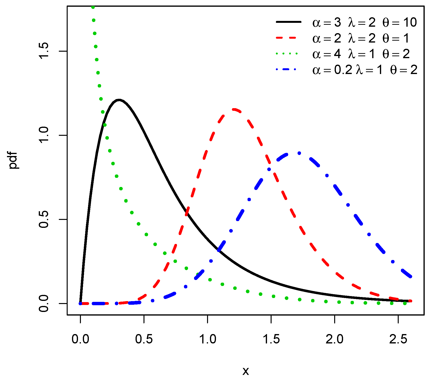
, which tends to 0 for all the values of the parameters. Numerical investigations of the critical points show that the TCPW distribution is mainly unimodal: only one maximum is reached.
Figure 1 illustrates the possible shapes for
by considering the following four sets of parameters as
:
,
,
and
. We see that
can be left, right skewed, near symmetrical and reverse J shaped.
The hrf of the TCPW distribution is obtained as
The following asymptotic properties hold. When , we get . Therefore, if , tends to , if , tends to , and if , tends to 0.
Also, when , we have . Hence, if , tends to 0, if , tends to , and if , tends to .
Numerical investigations of the critical points can be performed for
. For a visual approach,
Figure 2 illustrates the possible shapes for
by considering the following five sets of parameters as
:
,
,
,
and
. We notice again that the TCPW distribution is a very flexible distribution, having all possible monotonic and non-monotonic hazard rate shapes, such as increasing, decreasing, decreasing-increasing-decreasing, constant, bathtub and upside-down bathtub shapes.
After some algebra, the quantile function of the TCPW distribution is defined by
This tractable expression is an undeniable plus to simulate values from the TCPW distribution and to defined skewness and kurtosis measures, wherever the existence or not of moments. These points will be discussed later.
3. Notable Properties
In this section, some notable properties of the TCP-G family, and of the TCPW distribution in particular, are derived.
3.1. Linear Representations
Simple expansion series for the pdf and cdf of the TCP-G family are obtained according to the cdf and pdf of the exponentiated-G family by [
8] given by
and
, where
. The interest of such expansions series is mainly for practical purposes: the determination of some properties of the TCP-G family via such expansions can be more efficient than computing those directly by numerical integration involving the corresponding pdf (which is well-known to prone to rounding off errors).
Since
, owing to the well-known series decomposition of the arctangent function, we have the following series expansion for
:
Upon differentiation of
, a series expansion for
follows:
One can remark that the coefficients in these series expansions are readily computed numerically using any standard mathematical software. Also, in any numerical calculations using these series expansions, infinity should be substituted by a large integer number. In this sense, some properties of the exponentiated-G family can be useful to determine those of the TCP-G family, as developed for the moments and related functions in the next section.
In this study, we will use them to provide series expansions for the moments and related functions. Also, for a given baseline cdf
, we can go further these series expansions with more specific pdfs. For instance, for the TCPW distribution, owing to (
9) and the generalized binomial formula applied to
, we get
where
and
which is the survival function of the Weibull distribution with parameters
and
. Upon differentiation of
, we get
where
and
which is the pdf of the Weibull distribution with parameters
and
.
3.2. On Moments and Related Functions
Now, let
X be a random variable with the cdf given by (
1), defined on a probability space
.
By virtue of (
10), for any function
such that all the introduced quantities are well-defined, we have the following integral expression:
For some configurations, the integral term can be calculated or, at least, evaluated numerically by any mathematical software.
In particular, the
s-th moment of
X is obtained by choosing
, i.e.,
. Hence, by taking
, we get the mean of
X, i.e.,
. Furthermore, by taking
, we obtain
, from which we can express the variance of
X defined by
. From the first
s moments of
X, the
s-th central moment of
X can be deduced as
Then, some properties of the TCP-G family, as the skewness and kurtosis properties, can be investigated by the study of the s-th general coefficient of X given by .
The moment generation function of X according to t is obtained by choosing , i.e., . Similarly, the characteristic function of X according to t is obtained by choosing , where , i.e., .
Another important function is the
s-th incomplete moment of
X according to
y which follows from the choice
, where
denotes the indicator function equal to one if
A is satisfied and 0 otherwise, i.e.,
. In particular, the first incomplete moment allows us to define the mean deviation about the mean, i.e.,
, the mean deviation about the median, i.e.,
, as well as the Lorenz curve, the Gini inequality index and the Zenga curve, which are of great importance in many applied fields. Further details can be found in [
27,
28].
Let us now discuss some of the above properties in the context of the TCPW distribution, with the use of (
12). Thus,
X is a random variable following the TCPW distribution, i.e., having the cdf given by (
5). Then, the
s-th moment
exists. Owing to (
12) and
, where
, one can express it as
That is, we obtain the mean
and the variance
of
X proceeding as above. To illustrate the effect of the parameters
,
and
on them,
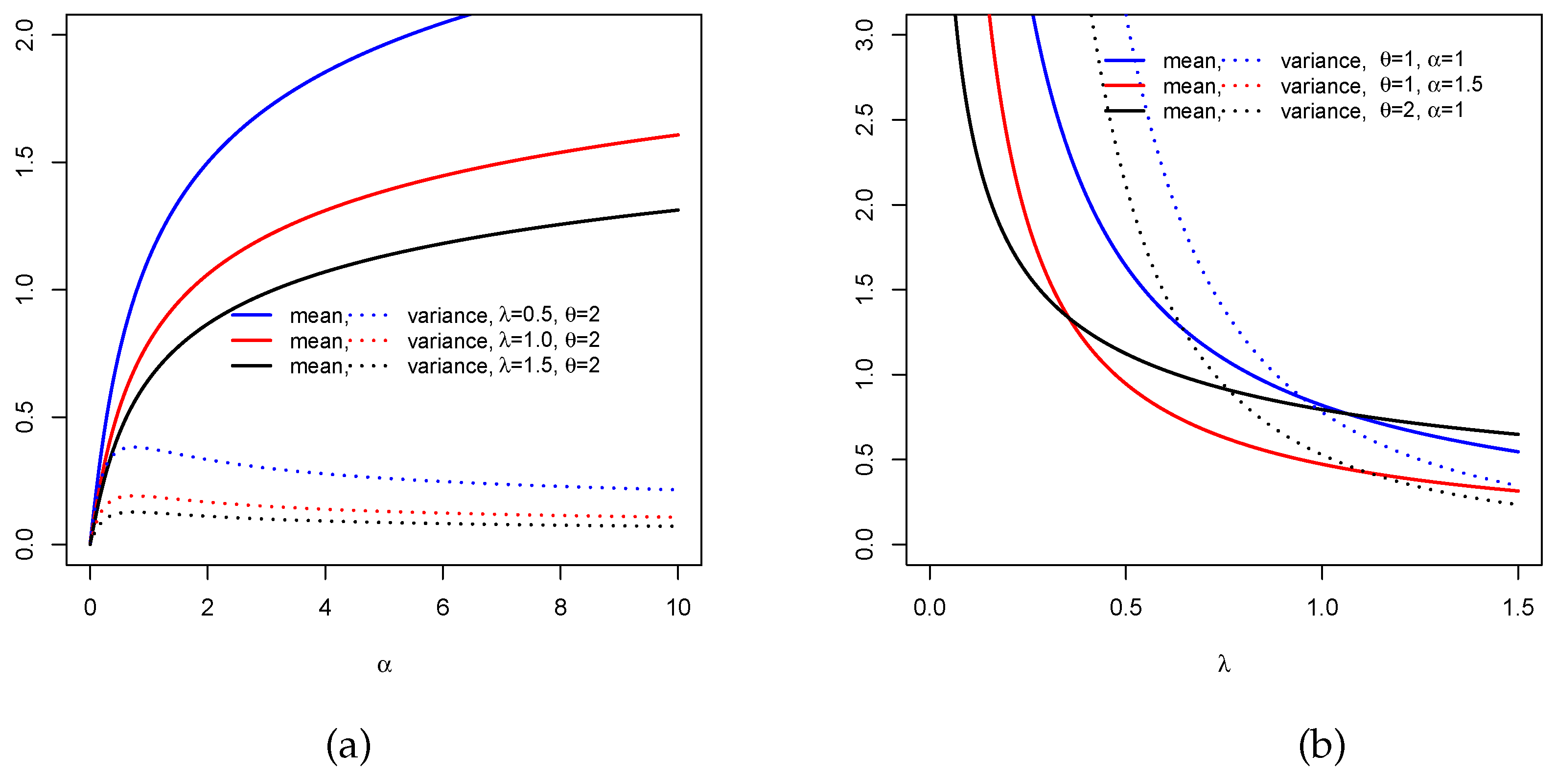
Figure 3 represents
and
under two different scenarios: (i) for fixed
and
and varying
and (ii) for fixed
and
and varying
. Wee that the mean can increase with a near constant variance (see
Figure 3a) whereas it can decrease with high variations for the variance (
Figure 3b). This illustrates the flexibility of these two measures according to the distribution parameters.
We conclude this part by the description of the incomplete moments of
X. By introducing the lower incomplete gamma function defined by
, the
s-th incomplete moment of
X is given by
Thus, the first incomplete moment can be derived, as well as the related important quantities and functions (mean deviations, Lorenz curve…).
3.3. Skewness and Kurtosis Based on Quantiles
As previously mentioned, one can define measures of skewness and kurtosis based on quantiles. In comparison to those defined with moments, they are more simple to calculate and not influenced by the eventual extreme tails of the distribution. One of the most useful skewness based on quantile is the MacGillivray skewness introduced by [
29]. In the context of the TCP-G family, based on (
4) and the median, it is given by the following function:
We can use this robust function to describe efficiently the effect of the parameters
on the skewness; more the shapes of the graphs of
are varying according to the parameters, more the skewness is flexible. One can notice that, for
, it becomes the Galton skewness studied by [
30]. The sign of the Galton skewness is informative on the right or symmetric or left skewed nature of the distribution;
means that the distribution is right skewed,
means that the distribution is symmetrical and
means that the distribution is left skewed.
Also, the kurtosis of the TCP-G family can be studied by considering the Moors kurtosis proposed by [
31]. It is defined by
A high value for means that the distribution has heavy tails and a small values for means that the distribution has light tails.
We now investigate the skewness and kurtosis of the TCPW distribution. In this case, thanks to (
8), the MacGillivray skewness and Moors kurtosis have a closed-form. We now propose some visual explorations of these measures.
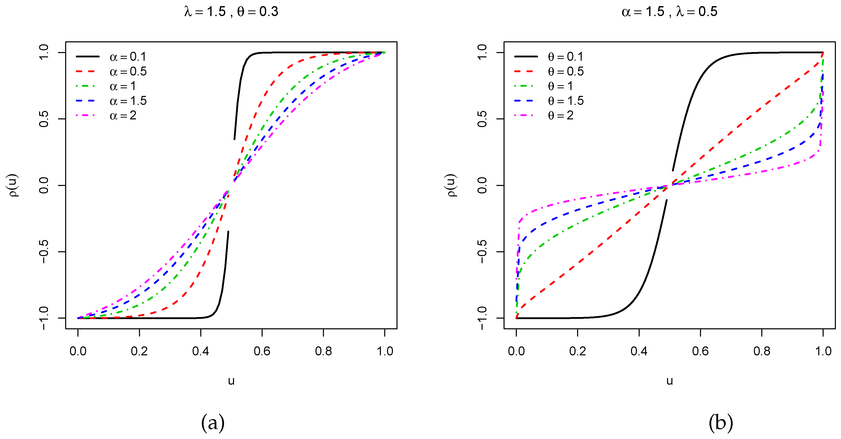
Figure 4 presents the MacGillivray skewness when (i)
and
are constant, i.e.,
and
, and
increases and (ii)
and
are constant, i.e.,
and
, and
increases. Moderate variations can be seen in the curves of
Figure 4a, meaning that the parameter
has a moderate effect on the skewness, whereas various wide variations on the shapes of the curves are observed in
Figure 4b, showing that the parameter
strongly influenced the skewness. Then, a similar visual approach is performed for the Galton skewness in
Figure 5. For the selected values of the parameters, we see that the Galton skewness decreases. Also, it is observed that it can be positive (see
Figure 5a) or negative (see
Figure 5b with
,
and
approximately), meaning that the TCPW distribution can be left or right skewed, respectively.
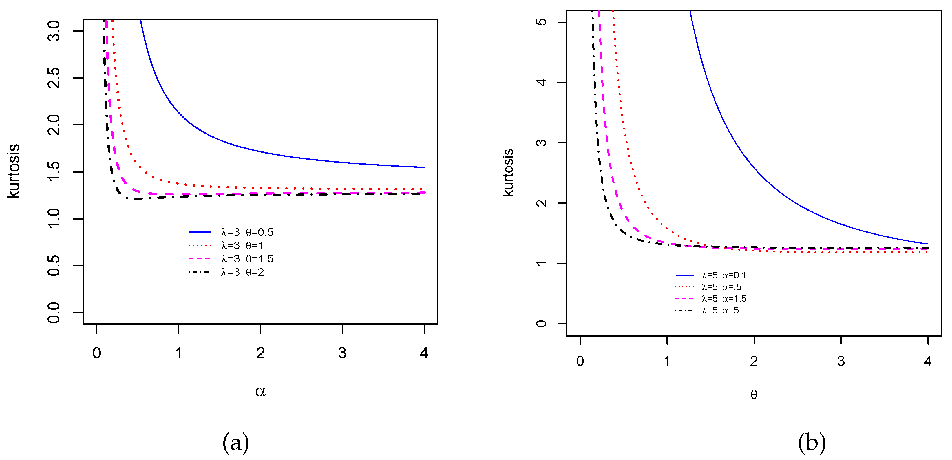
Figure 6 displays the Moors kurtosis following the same scenarios. We see that the TCPW distribution can be of different kurtosis nature, which small or high possible values. All these facts show the great skewness and kurtosis flexibility of the TCPW distribution.
3.4. Rényi Entropy and q-Entropy
Entropy is a fundamental measure to quantify the amount of informations in a distribution, finding applications in information science, thermodynamics and statistical physics. Here, we investigate two different and complementary kinds of entropy arising from various physical experiments: Rényi entropy and
q-entropy, of the TCP-G family, as introduced by [
32,
33], respectively. As common interpretation, the lower the entropy, the lower the randomness of the related system. For further detail, we refer the reader to the survey of [
34].
Rényi entropy is defined by
with
. Since it can be expressed analytically, we aims to provide a series expansion of
. Owing to (
2) and the generalized binomial formula, we get
Therefore, we can expressed
as:
For given functions and parameters, mathematical software can be useful to evaluated numerically this last integral.
If we consider the case of the TCPW distribution, we can formulate
by the above expression and the following series expansion:
In the general context of the TCP-G family, the
q-entropy is defined by
with
. Proceeding as for the Rényi entropy, we can expressed it as:
For the the TCPW distribution, by replacing
by
q, we can express the integral term as in (
13).
3.5. Order Statistics
We now present the main properties of the order statistics in the context of the TCP-G family. The general theory can be found in [
35].
Now, let
be a random sample from the TCP-G family and
be the
i-th order statistic, i.e., its
i-th smallest random variables (in the standard probabilistic ordering sense, i.e.,
if and only if
). Then, it is well-known that the cdf and pdf of
are, respectively, given by
and
We now focus on the determination of a tractable series expansions for
and
. In this regard, let us now present a result on the series expansion for the exponentiated arctangent function with power integer. For any
and any integer
s, we have
where
and, for any
,
is defined by the following relation:
(thus, for instance,
and
). The proof of this intermediary result is discussed below. Owing to [
26] (Point 0.314), for an integer
s, a sequence of real numbers
and
, by assuming that the introduced sums converge, we have
, where the coefficients
are determined by the following relations:
and, for any
,
. Since, for any
, we have
, with
(so
), the above result implies that
Thus, it follows from (
15) that
where
(
is defined as in (
15) with
). This shows that the cdf of the order statistics of the TCP-G family can be expressed as an infinite mixture of cdfs of the exponentiated-G family by [
8]. Therefore, the well-established properties of the exponentiated-G family can be used to determine those of the order statistics of the TCP-G family. Indeed, from
, one can deduce the corresponding pdf by differentiation as follows:
This expression allows determining moments, skewness, kurtosis, and other important measures and functions.
In the case of the TCPW distribution, a refinement of these series expansions are possible. Indeed, we can expend
in a series expansion as in (
11), which implies that
where
and
(we recall that it is the survival function of the Weibull distribution with parameters
and
).
Also, upon differentiation of
, the pdf of
is given by
where
(we recall that it is the pdf of the Weibull distribution with parameters
and
). As a direct application, the
r-th moment of
can be obtained as
5. Application to Two Practical Data Sets
The TCPW model finds a concrete interest in the precise modelling of real life data sets. Here, we illustrate this aspect by considering the two following data sets.
The first data set is taken from tests on the endurance of deep-groove ball bearings. The measurements represent the number of millions revolutions reached by each bearing before fatigue failure (see [
37]). The first data set is given by: 17.88, 45.60, 54.12, 68.88, 105.84, 28.92, 48.40, 55.56, 84.12, 127.92, 33.00, 51.84, 67.80, 93.12, 128.04, 41.52, 51.96, 68.64, 98.64, 173.40, 42.12, 54.12, 68.64, 105.12. A basic statistical description of this data set is proposed in
Table 9.
From
Table 10, we observe that the data are right skewed with a moderate kurtosis, which corresponds to a case covered by the TCPW model.
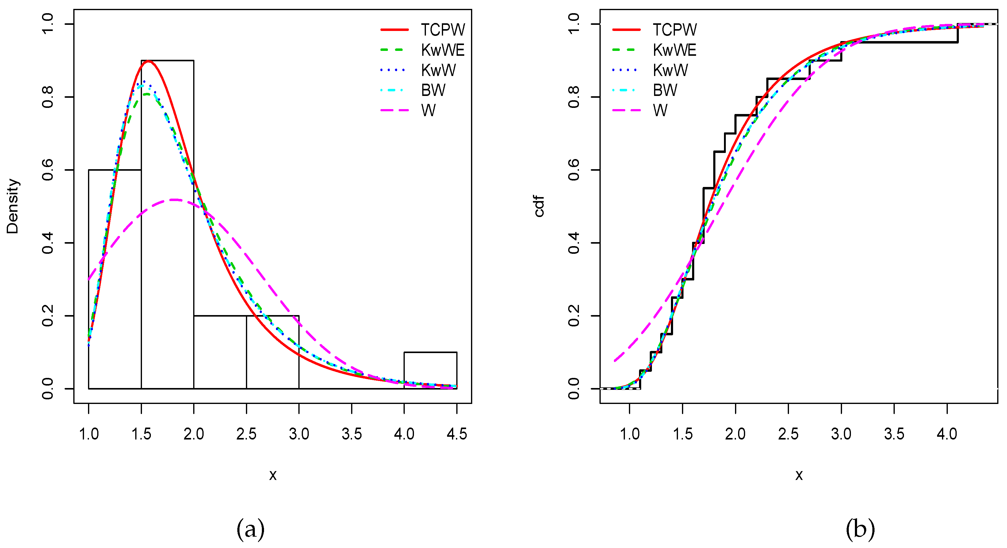
The second data set refers to a lifetime data set taken from [
38] (p 105). The data are: 1.1, 1.4, 1.3, 1.7, 1.9, 1.8, 1.6, 2.2, 1.7, 2.7, 4.1, 1.8, 1.5, 1.2, 1.4, 3, 1.7, 2.3, 1.6, 2. A first statistical description of this data set is presented in
Table 10.
From
Table 10, we see that the data are highly right skewed with a consequent kurtosis, which is a case also covered by the TCPW model.
Then, we compare the TCPW model to the following well-established models: the Kumaraswamy–Weibull-exponential (KwWE) model by [
39], the Kumaraswamy–Weibull (Kw-W) model by [
9], the beta Weibull (BW) model by [
40], and the standard Weibull (W) model. The results are obtained using the R software.
By respecting the standard in the field, all the parameters will be estimated by the MLEs in the SRS case, even if the simulation study is favorable to the RSS for the TCPW model (see the subsection above). Then, standard measures are taken into account, namely: the Cramér-Von Mises (CVM) statistic, the Anderson-Darling (AD) statistic and the Kolmogorov-Smirnov (KS) statistic along with the corresponding
p-value. The obtained results are summarized in
Table 11 and
Table 12 for the first and second data sets, respectively. We see that the TCPW model has the smallest CVM, AD, KS and the greatest
p-value (with
p-value
and
for the first and second data sets, respectively, which are quite close to the limit 1), attesting that it is the best model for these data sets.
To solidify this claim, we provide the minus estimated log-likelihood function (
), Akaike information criterion (AIC), corrected Akaike information criterion (CAIC), Bayesian information criterion (BIC), and Hannan–Quinn information criterion (HQIC) in
Table 13 and
Table 14 for the first and second data sets, respectively. We observe that the TCPW model has the smallest AIC, CAIC, BIC and HQIC, attesting its superiority in terms of modelling. To illustrate this,
Figure 7 and
Figure 8 show the fits of (i) the estimated pdfs over the corresponding histograms and (ii) cdfs over the corresponding empirical cdfs of the related models, for the first and second data sets, respectively. As expected, nice fits can be seen for the TCPW model.
6. Concluding Remarks and Perspectives
In this paper, we offered a new general family of distributions based on the truncated Cauchy distribution and the exp-G family, called the truncated Cauchy power-G (TCP-G) family. A focus was put on the special member of the family defined with the Weibull distribution as baseline, called the TCPW distribution. Its cdf has the feature of being simply defined with the arctangent and power functions, allowing tractable expressions for the other corresponding functions (pdf, hrf, qf…). In addition to its simplicity, we revealed the desirable properties of the family, such as very flexible shapes for the pdf and hrf, skewness, kurtosis, moments, entropy…. By considering the special TCPW model, a full simulation study illustrates the nice performance of the maximum likelihood method in the estimation of the model parameters. The deep analysis of two famous data sets shows all the potential of the new family, with fair and favorable comparison to well-established models in the same setting.
From the perspective of this work, one can apply the TCP-G family in a regression model framework (creating new possible distributions on the error term). Also, one can investigate some natural (and not too complicated) extensions of the TCP-G family as those defined by
the cdf given by
where
, which corresponds to the exponentiated cdf of the TCP-G family,
the cdf given by
where
,
and
denotes the cdf of a univariate continuous distributions with parameter vector denoted by
.
These extensions needs further investigations; there is no guarantee as to their superior efficiency over the former TCP-G family is provided at this stage, opening new work chapters for the future.

 ,
, 


