1. Introduction
Multistability is a widespread phenomenon in the field of dynamical systems where a system exhibits multiple stable states or more generally attractors [
1]. Appearing in nearly all disciplines of natural science and engineering, including biology [
2,
3], chemistry [
4,
5], electronics [
6,
7], fluid mechanics [
8,
9], genetics [
10,
11], and physics [
12,
13], researchers have shown substantial interest in such behavior [
1]. In neuroscience, computations are thought to be implemented by multistable dynamical systems, and recent experimental and methodological advances have generated renewed interests [
14,
15,
16,
17,
18,
19]. The multiple attractors within these dynamical systems seem to underlie a wide array of functions, including sensory perception [
20], motor function [
21], and cognition [
22,
23], as well as dysfunctions, such as movement disorders [
24], epilepsy [
25], and disorders of consciousness [
26,
27]. We hypothesized that multistability underlie some dynamical neurological diseases such that manifested symptoms are fundamentally due to the inability to naturally transition from one basin of attraction to another. Under this hypothesis, neurostimulation techniques provide a means to perturb neural systems to assist transition between attractors as a treatment option.
Open-loop electrical stimulation therapies have shown remarkable successes, most notably with Parkinson’s disease [
28]. However, open-loop strategies are likely to be insufficient for the general induction of attractor transitions that manifest complex nonlinear dynamics and non-trivial stimulus induced perturbations. For example, high-amplitude low-frequency signals, such as those dominant in disorders of consciousness [
27], suggest the existence of strong attractor dynamics which may require a sophisticated feedback control system to transition out [
29]. This sets the stage for the next-generation closed-loop neural stimulators that can intelligently learn to induce attractor transitions. The added complexity of the closed-loop stimulation systems calls for a platform to develop and test their efficacy.
In this paper, we aimed to develop a hardware platform by which these intelligent stimulation algorithms could be tested and validated on. Clinically, this platform can serve as an initial stepping stone, prior to the use of animal models and human patients, in demonstrating the successful use of a stimulation regime under our hypothesis for a given application. As is a common method for realizing a dynamical system physically, an analog electronic circuit exhibiting the desired dynamics is constructed [
30,
31,
32]. Due to the nature of widely used electrical stimulation for neurological implants, this medium will serve well as a testbed. While such a system can be developed as a software package, neurostimulators have an analog interface, where typically current is injected into the neural tissue. By keeping our platform entirely analog, we maintain this interface. Furthermore, the analog nature of the brain ensures the existence of inherent noise and imperfections in the system dynamics. We would like to implement these imperfections here as a result of the medium by which the platform is designed on, rather than needing to over-complicate our model. This added variability will require a stimulation algorithm to be more robust.
To reduce unnecessary complexity, we constructed our system to demonstrate the simplest form of oscillatory multistability, birhythmicy. More specifically, the system will simultaneously exhibit two self-exciting limit cycles of notably different frequencies. Given that the state of the system is sufficiently close to one of the two attractors, an intelligent stimulation algorithm can be tested by trying to perturb the system into the other basin of attraction. While this may seem like a substantial simplification of global brain dynamics for typical neurological function, when viewing brain activity at different spatiotemporal scales under specific conditions far fewer attracting states may be present. Two examples are patients under deep anesthesia or within a comatose state. Under such conditions, there appears to be coherent synchronization across large brain regions [
26,
27]. Such homogeneity would vastly simplify the underlying dynamic behavior, resulting in far fewer attractors. Under the right lens, our developed model becomes more immediately applicable.
In the following section, we derive the system from the general continuous-time dynamical system underlying the gated recurrent unit (GRU), a commonly used recurrent neural network architecture [
33,
34]. In
Section 3, we discuss the details of the circuit design and present the results of the physical realization. In
Section 4, we discuss the addition and design of a nonlinear circuit, state dependent on the system described in
Section 2 and
Section 3, by which external stimulation is interfaced. The addition of this nonlinear
stimulator circuit will ensure random or periodic stimulation patterns will be ineffective in inducing transitions between the two attractor states.
2. Birhythmic Dynamics in 3-Dimensions
Our goal was to find a simple bistable dynamical system where each attractor corresponds to a periodic orbit. We draw from the recurrent neural network literature on simple forms of stable limit cycles. Specifically, we utilize the autonomous continuous-time gated recurrent unit (ct-GRU) [
33,
34] formulation, which can be represented as follows:
where
is the state of the system,
are the parameter matrices,
are the bias vectors, ⊙ represents the Hadamard product, and
is the element-wise logistic sigmoid function. For a given set of parameters, fixed points of the system exist where
. Since
, this term does not influence the roots of the right-hand side of Equation (
1). Therefore,
can only affect the speed of the flow and, in turn, can be neglected when choosing a set of parameters for the system to enact a desired structure of attractors [
34]. Note that, if the parameters of
have been set to zero, the ct-GRU architecture simplifies to the classic ct-tanh-RNN if the parameters of
are also set to zero.
In previous work [
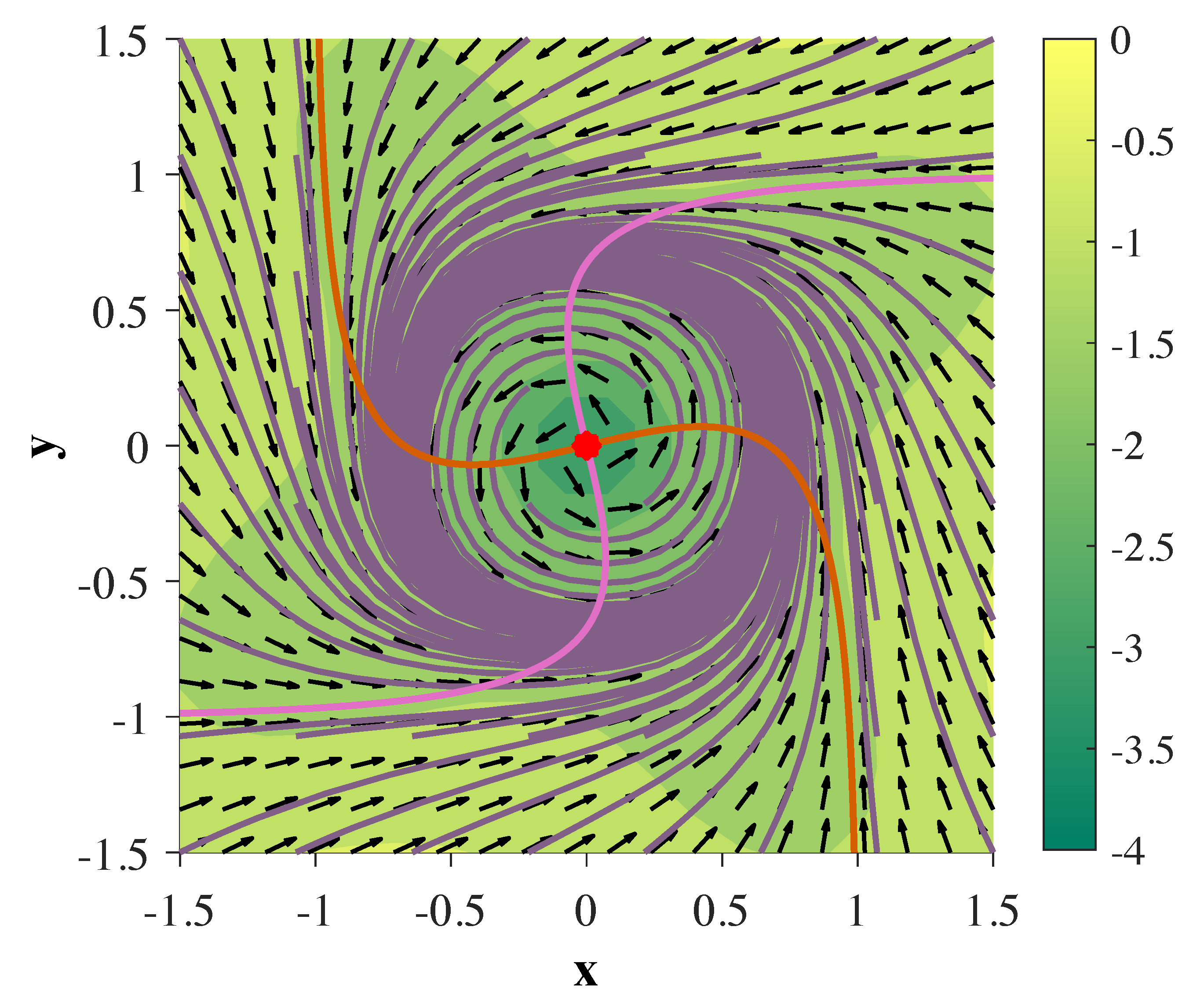
34], we have shown that, for
, the ct-GRU is capable of expressing a single limit cycle (attracting closed orbit) in phase space under the following set of parameters:
where
and
. The phase portrait depicting this behavior for
can be seen in
Figure 1, where
.
Extending the system to 3-dimensions allows for the simultaneous existence of two limit cycles in phase space under a single set of parameters. More specifically, the addition of a third dimension enables us to mirror any attractor structure representable for
across an unstable manifold on the plane defined by the original two dimensions in
. This behavior is depicted in
Figure 2A, where now
, and the parameters are set as follows:
As stated before, only acts to adjust the speed of phase flow. If , the periods of both limit cycles are equal. As a means to easily decouple the two frequencies of oscillation, the velocity of flow may be made dependent on its vertical position with respect to the z-axis. While the range of the logistic sigmoid function has the benefit of always being defined on , it may produce inaccurate results when physically realized along its tails. Furthermore, any function that is strictly positive and sufficiently well-behaved on the region of phase space we are interested in will work under this context.
For simplicity, we redefine
linearly as
. We then note that Equation () is asymptotically bound to
. To account for potential error in the electronic realization, we set
such that its output remains strictly positive on
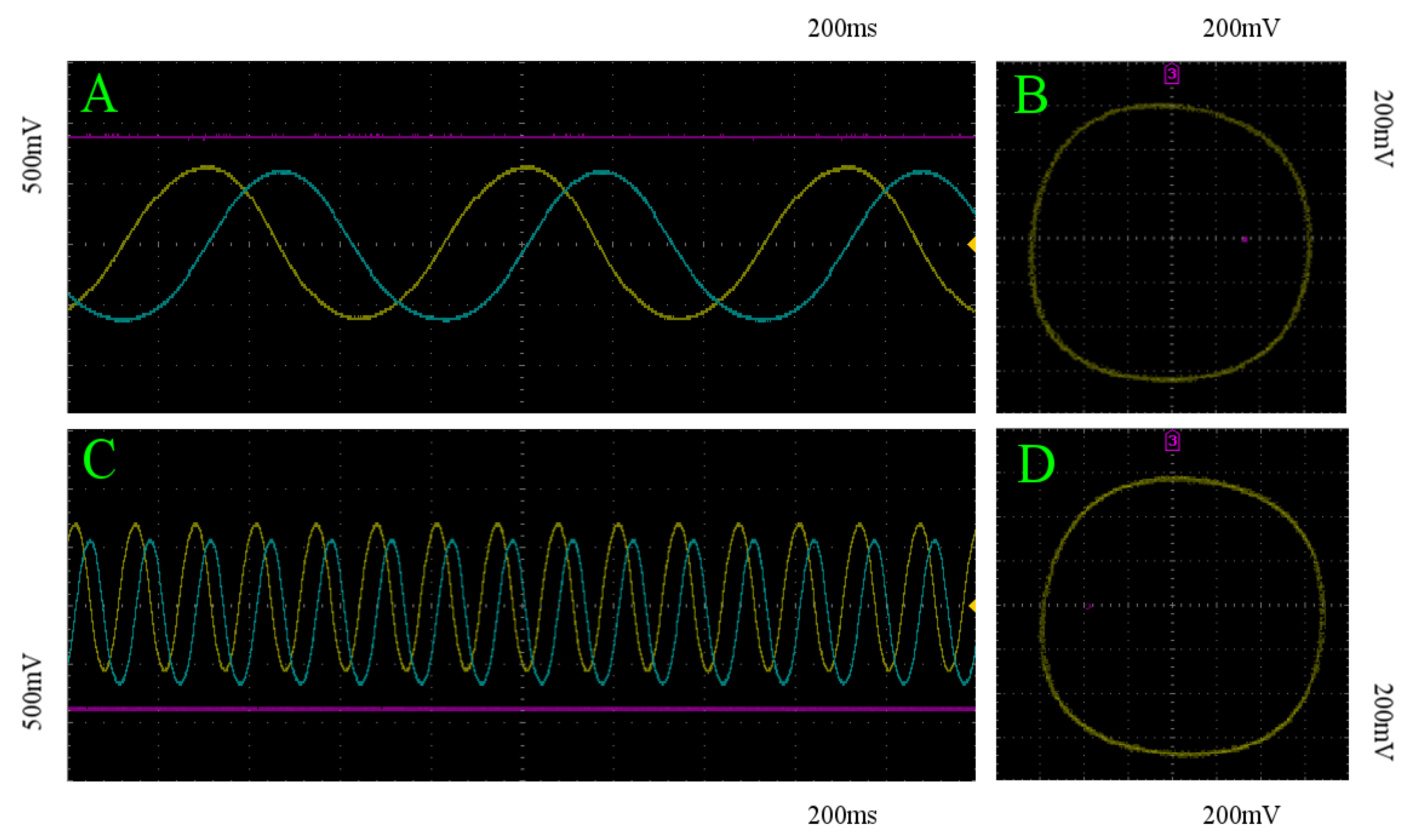
. The results of this linear update-gate are demonstrated in
Figure 2B,C and achieved under the following set of parameters in conjunction with those of Equation (
6):
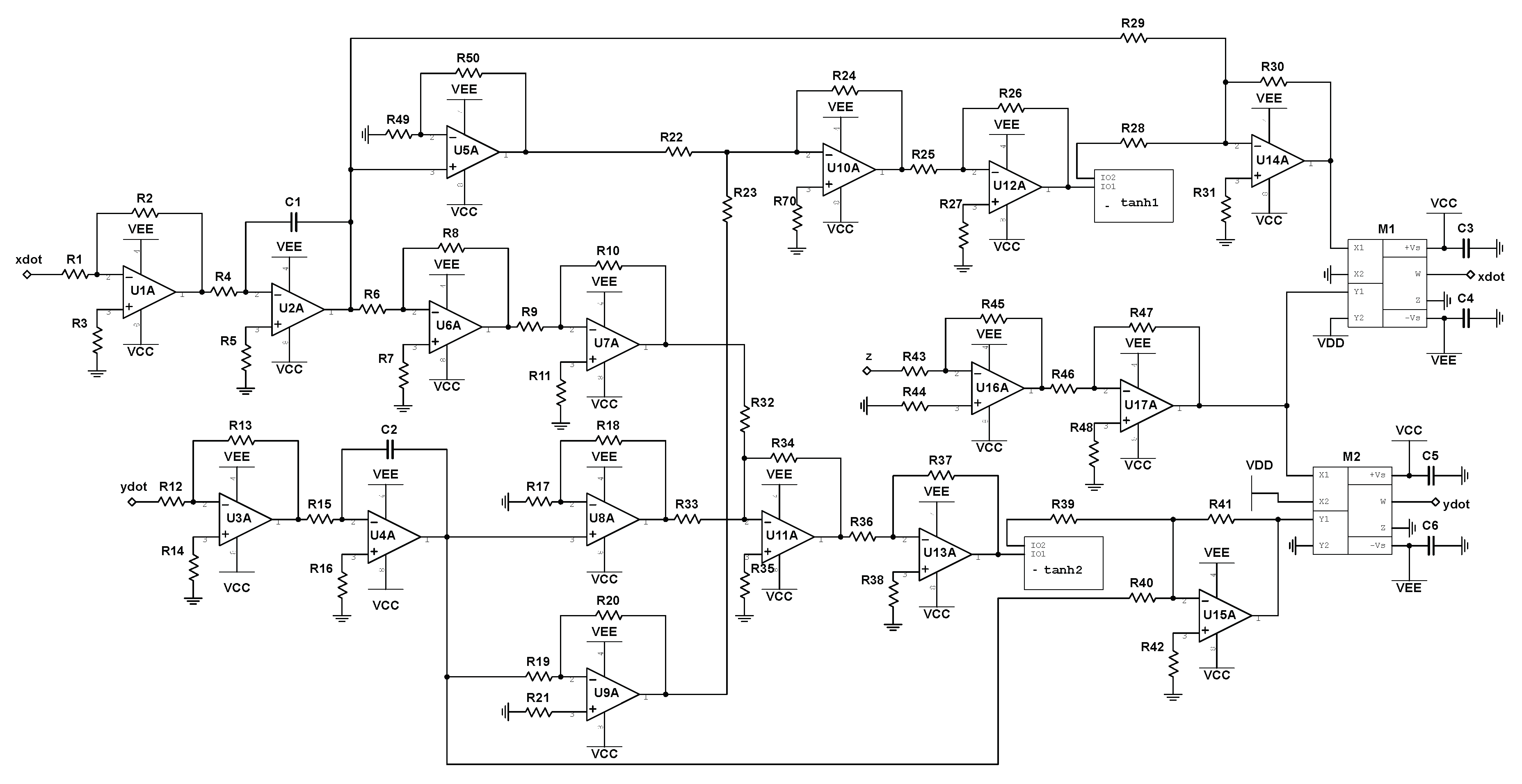
To better grasp the dynamical system depicted in
Figure 2 to be later realized, we can rewrite Equations (
1)–(4) explicitly in terms of
and
z with our chosen parameters from Equations (
6) and (
7) as follows:
where
is an added time constant that will be implemented in the circuit realization to adjust the difficulty of transitioning between attracting states. For our implementation of Equations (
8)–(10), we let
.
4. Nonlinear Stimulator Circuit Design and Discussion
When looking at the system derived in
Section 2, as expressed by Equations (
8)–(10), we notice the geometric simplicity of the global dynamics. As shown in
Figure 2A, the two periodic attractors are mirror images of one another across a planar unstable manifold on the x-y plane. This symmetry enabled us to easily decouple the frequencies of each limit cycle by introducing a strictly positive variable time constant dependent only on our
z-coordinate. However, this introduces a clear problem from the point of view of developing a neurostimulation testbed. In order to transition between basins of attraction, we only need to worry about the component
. In other words, transition between attractors can be achieved with constant stimulation on
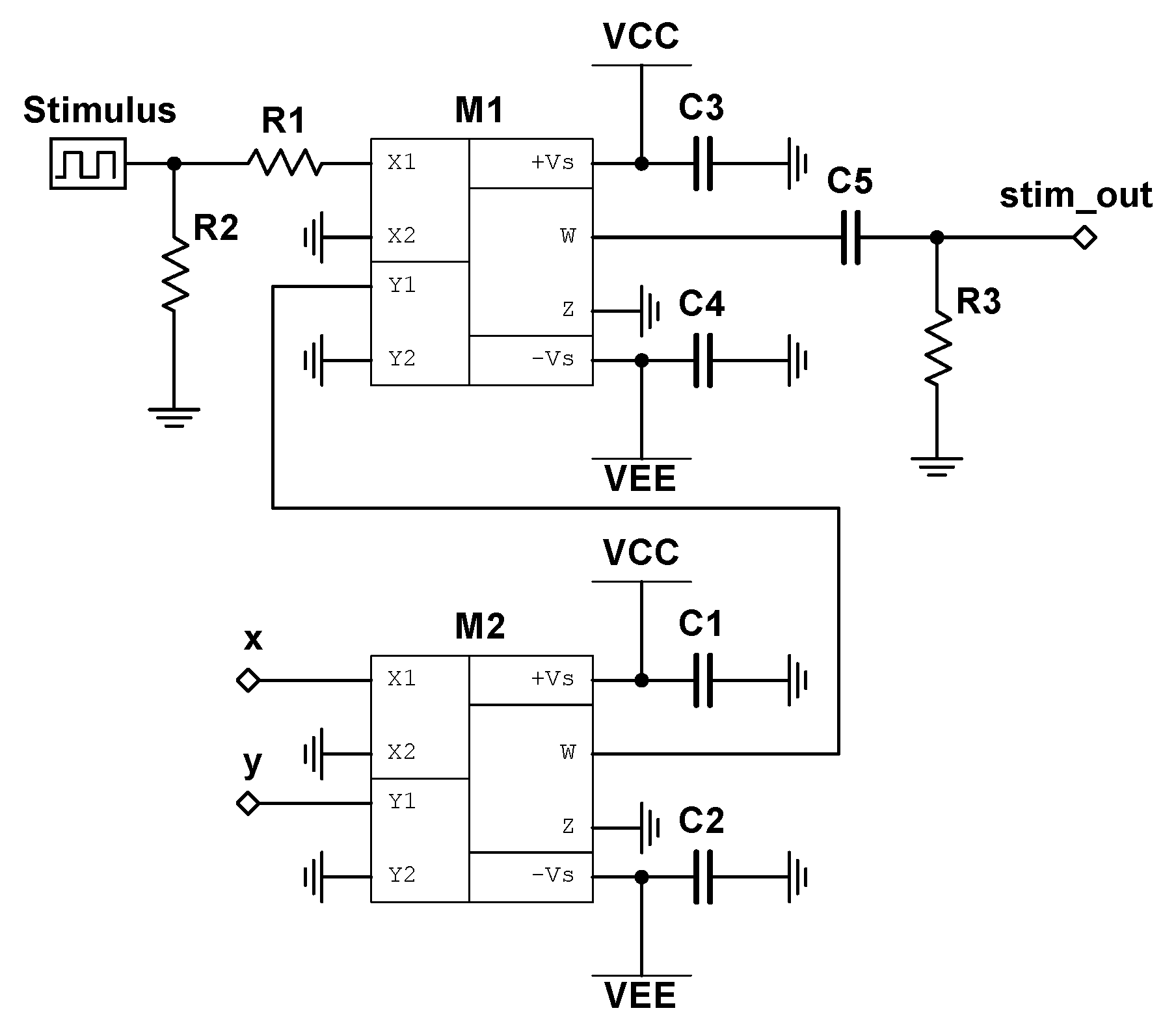
z. This solution to attractor transition is trivial, and does not require the use of an intelligent algorithm to solve, rendering it inadequate as a testbed. In order to negate this issue, we develop a state-dependent nonlinear stimulator interface circuit by which all stimulus must pass through. In addition, we allow only one location of stimulation within the circuit previously designed, as marked by the node labeled
stim_out in
Figure 4, where the output to the stimulator circuit will be fed in and summed with the current value of
in the system. By extending the system properly in this way, we can prevent straightforward stimulation patterns (i.e., constant, random, periodic, etc.) from inducing attractor transitions.
Ideally, we want to develop a stimulation circuit such that a pulse stimulated at a random time may cause the output, stim_out, to either increase or decrease. Furthermore, the amount by which the signal can change should exist on a continuum, rather than outputting a voltage from a finite set of values. The final requirement we will enforce for such a circuit will be that a stimulation pulse delivered at a random time should have equal probability of increasing or decreasing the output signal. This last requirement ensures that if one stimulates randomly or continuously, the expected value of stim_out averaged across all time will be zero as time approaches infinity.
Due to the sinusoidal nature of the
x and
y components in Equations (
8) and (9), Equation (
12) will serve as the input/output relation of the stimulator circuit at a given time
t.
where
is the output voltage of the stimulator circuit, and
is the input stimulus (note that
when no stimulus is applied). We note that this system satisfies all of our requirements, as
z is independent of
x and
y. To transition from the slow limit cycle to the fast limit cycle, stimulation must be applied primarily when
and
are of opposite signs. By doing this, the rate of change in
can be made negative on a subset of these intervals (dependent on the current value of
). Assuming that this downward forcing of
can both overcome the pullback from the attractor during these intervals and travel further downward than the accumulated upward travel during periods of no stimulation, then, after a sufficient amount of time, the system will jump over the unstable manifold at
and into the basin of attraction of the fast limit cycle. Since the speed of oscillation is dependent on
, any added stimulation will change the time window by which proper stimulation should be applied, ensuring that a periodic stimulation regime will fail to transition between the attractors. By the same argument, to transition from the fast limit cycle to the slow limit cycle, stimulation must be applied primarily when
and
are of the same sign.
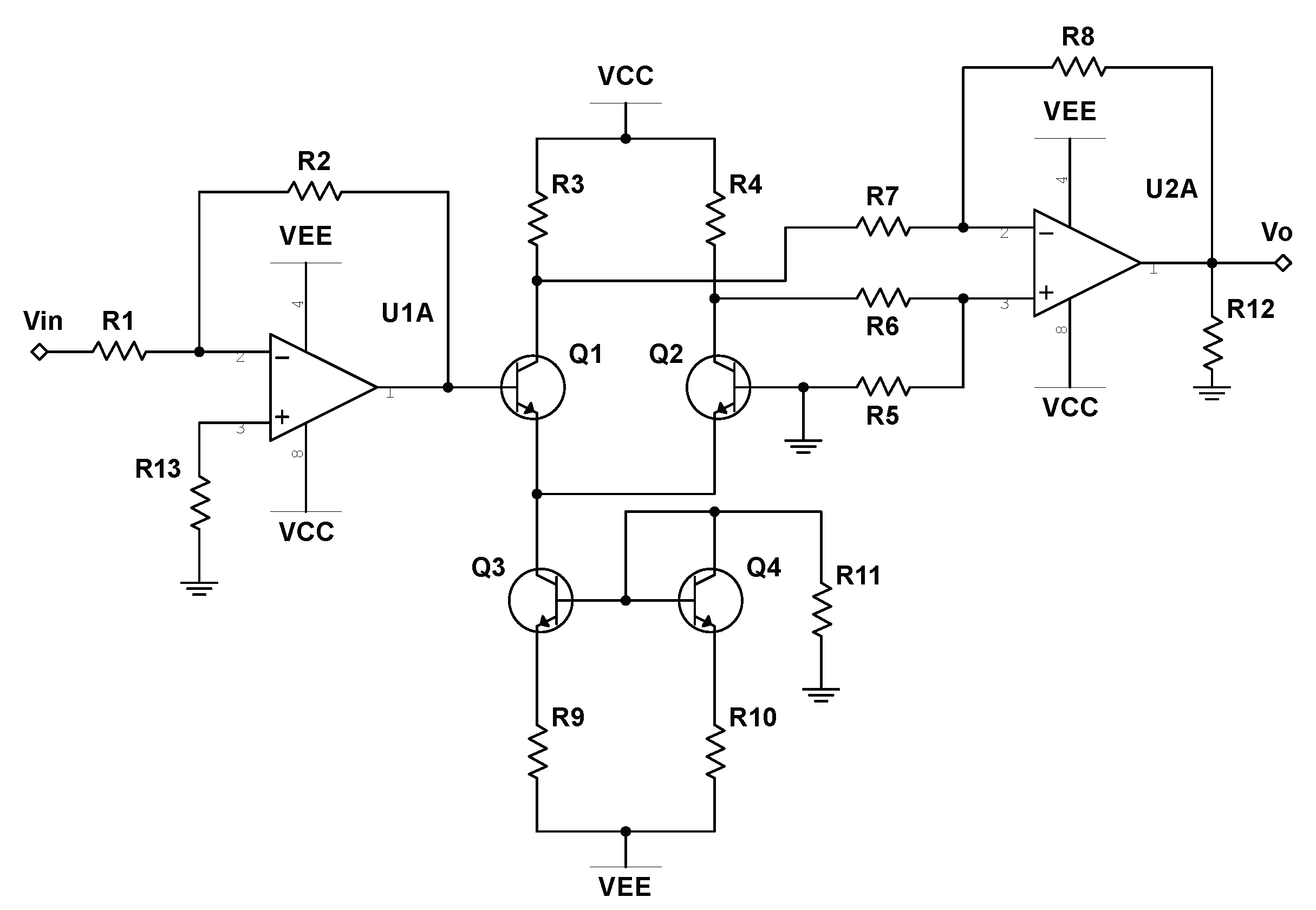
Figure 8 depicts the schematic for the described stimulator circuit, where
is labeled as
Stimulus.
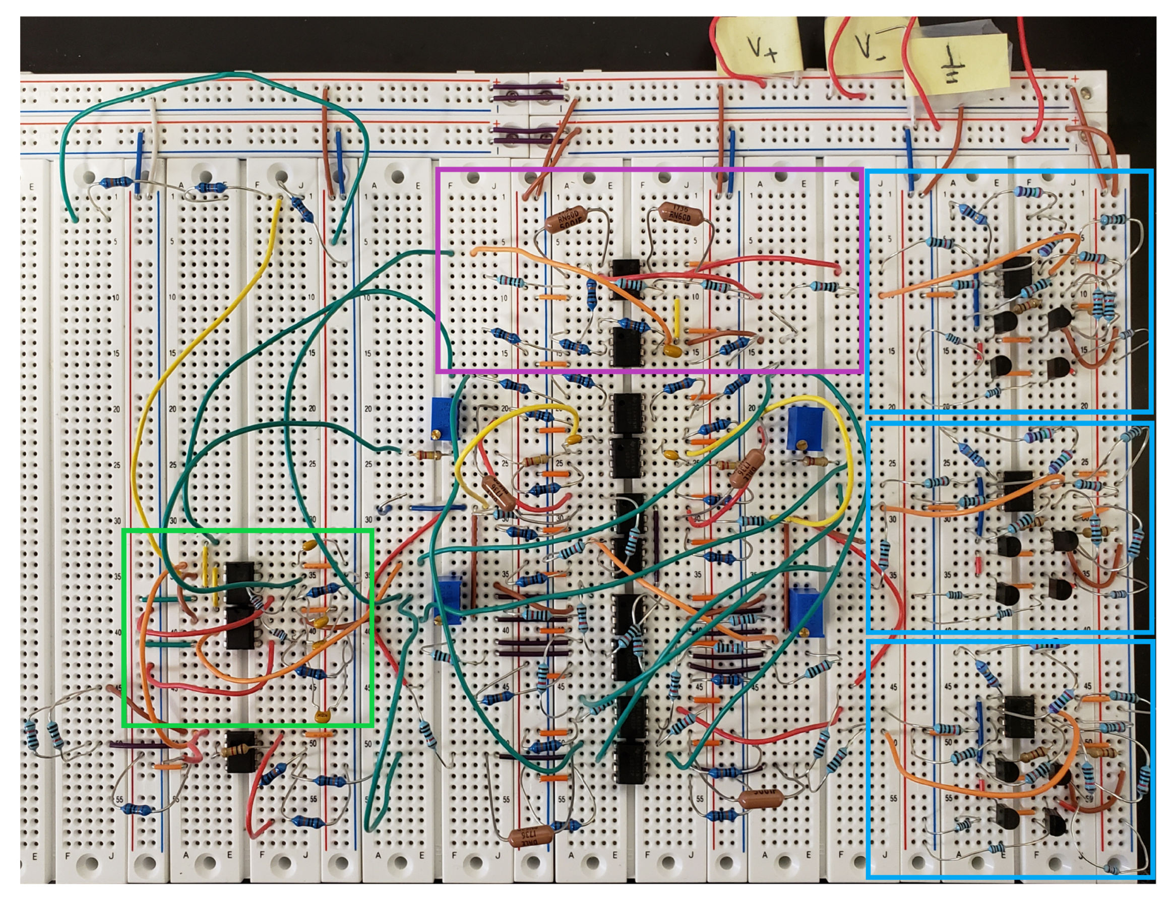
A physical realization of the stimulator circuit was created in conjunction with the birhythmic system and tested with a stimulus that could be turned on (4 V) or off (0 V). While this voltage range is certainly larger than those seen during neurostimulation, we note that this testbed acts to validate the underlying logic of a stimulation algorithm, and that this range is made proportional, in a practical sense, to the voltage range of the constructed dynamics. For interfacing with a traditional neural stimulation device, an additional signal amplifying circuit will need to be constructed to take in stimulus (typically low current biphasic pulse injections), and control a properly scaled voltage output which will be fed into the input of our designed nonlinear stimulator circuit.
In order to test the validity of our constructed system we recorded twenty trials for each of several stimulation methods, where half of the trials had the state of the system initialized on the slow limit cycle, and the other half of the trials were initialized on the fast limit cycle. Each trial was recorded for five seconds. We show that neither 4 V constant stimulation nor 4 V manually random stimulation induce state transition, and that these results appear invariant to the initial phase angle of the oscillations in and when stimulation is applied. Furthermore, we implement a stimulation pattern that can successfully transition between the stable limit cycles.
For constant stimulation, we statistically quantify the expectation of the maximum euclidean distance
moves away from the limit cycle that the system is initialized on for a given trial. The
z coordinates of both limit cycles empirically derived in
Section 3.3 will be used. In the case of the slow limit cycle, the sample mean of the maximum distances achieved on each trial is
V, with a standard deviation of
V across trials, implying that each trial was nearly identical in its effectiveness to transition between states. For the fast limit cycle, this sample mean is
V, and no variance was detectable in these recordings in 24-bit resolution. A
s segment of
for all trials is depicted in
Figure 9, where constant stimulation is denoted in turquoise.
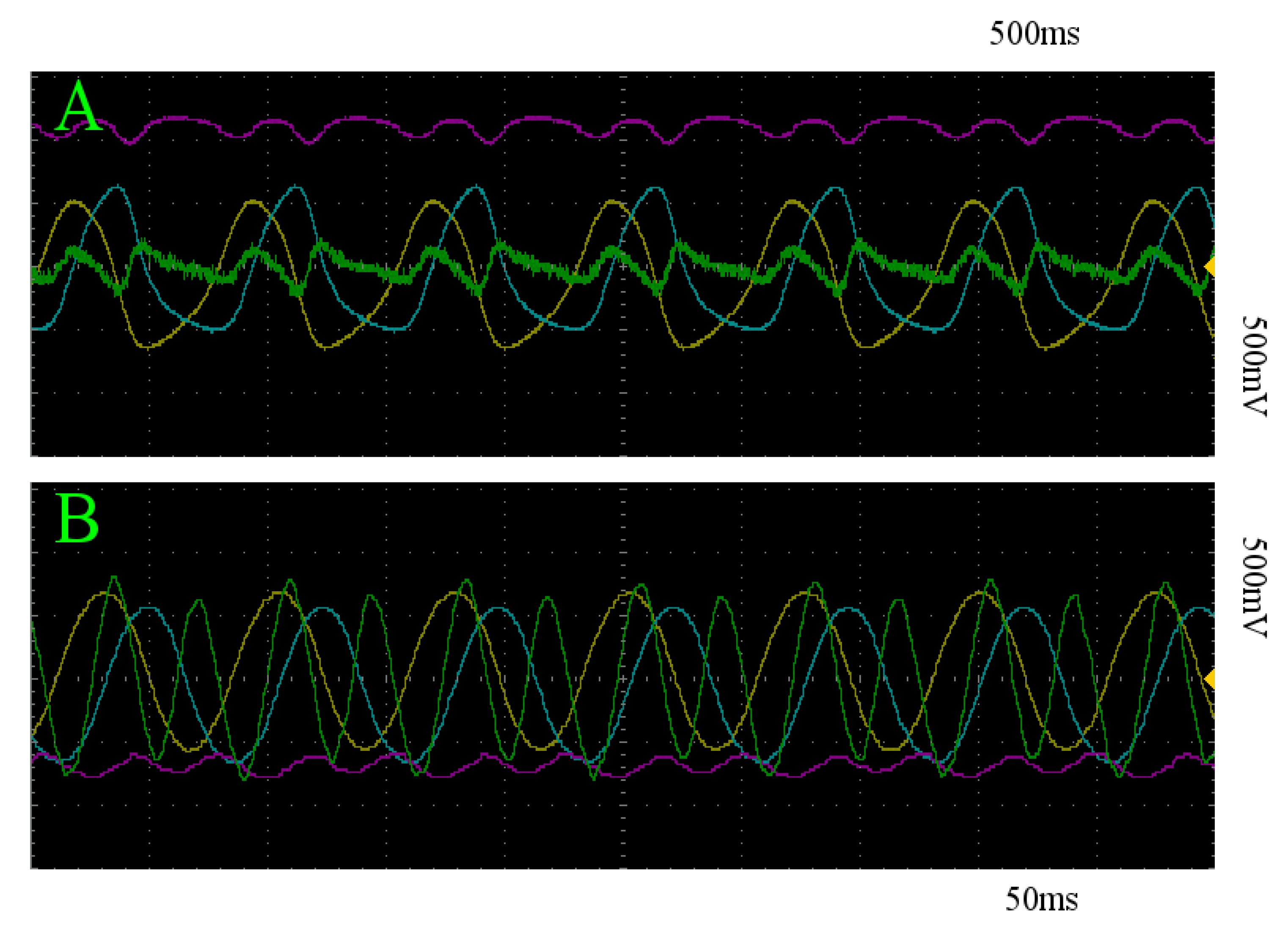
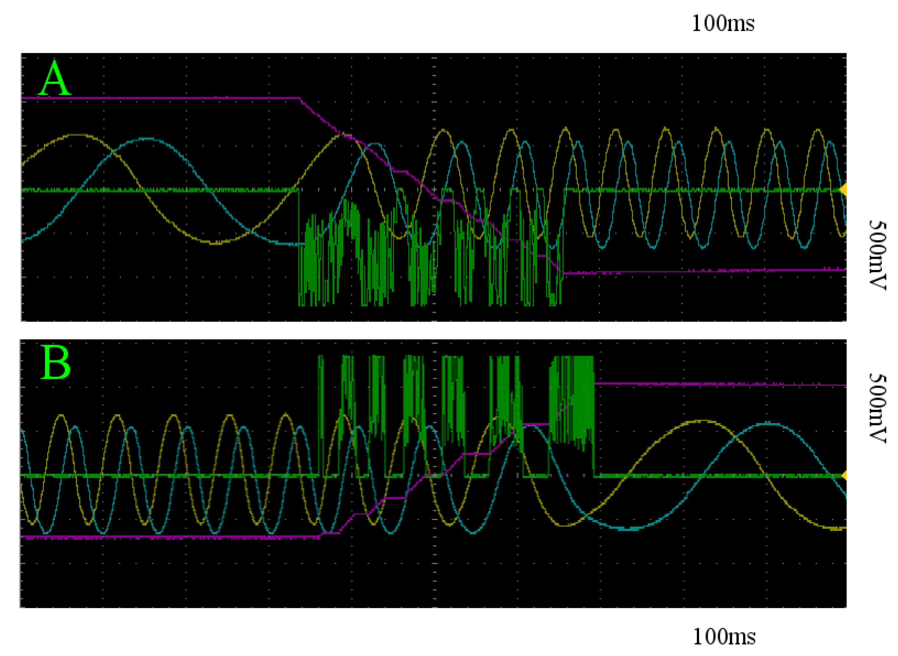
Figure 10A,B depict an example of the resultant behavior of the system under constant 4 V stimulation initialized on the slow and fast limit cycles, respectively. The yellow, blue, and pink curves represent the
x,
y, and
z components of the system, and the green curve depicts the voltage over time of
stim_out.
For random stimulation, we do the same thing. In the case of the slow limit cycle, the sample mean of the maximum distance achieved on each trial is
V, with a standard deviation of
V across trials. For the fast limit cycle, this sample mean is
V, with standard deviation of
V across trials. A segment of
for all of these trials is depicted in orange in
Figure 9.
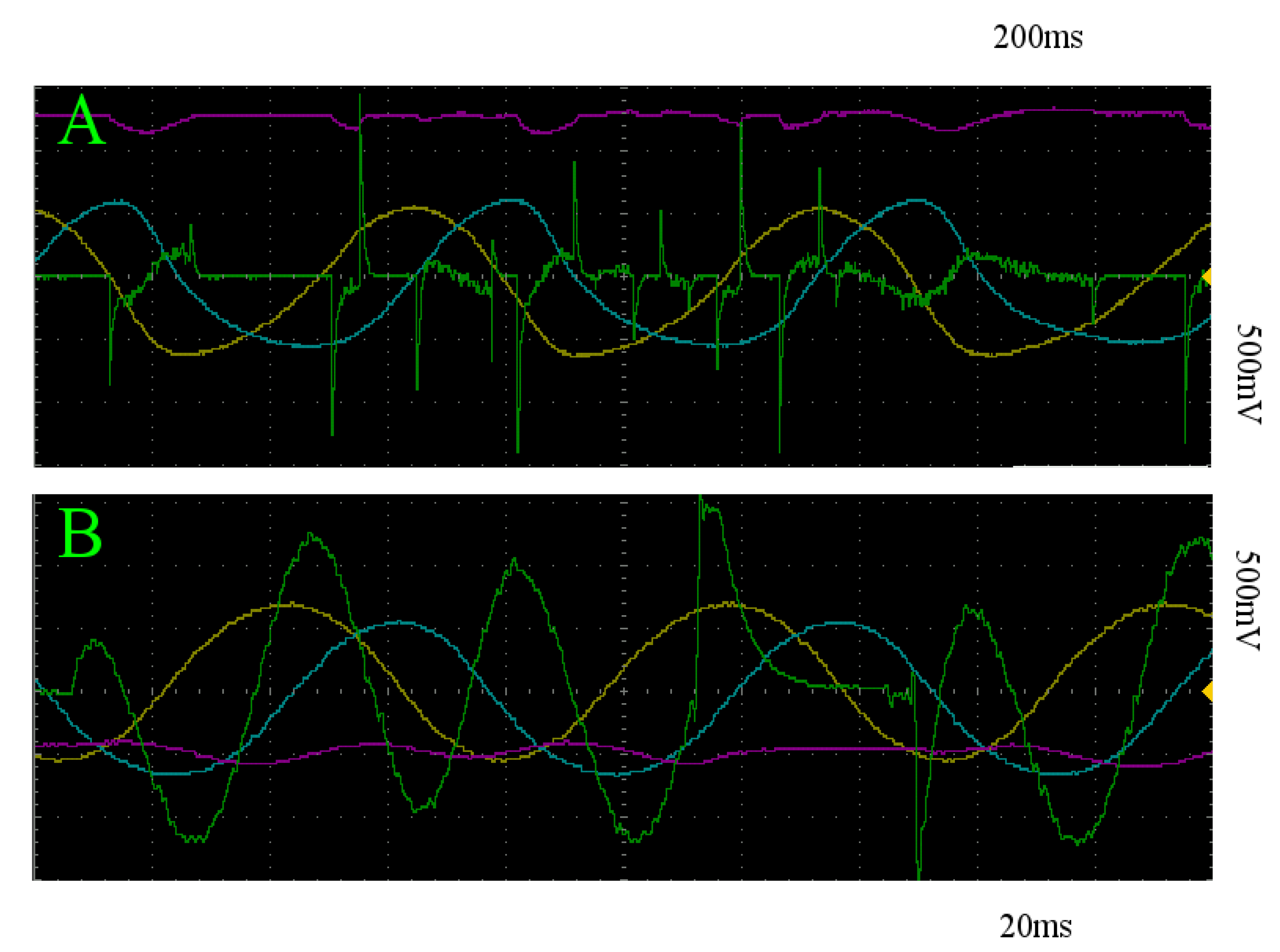
Figure 11A,B depict an example of the resultant behavior for trajectories initialized on the slow and fast limit cycles, respectively.
Despite executing stimulation at a random initial phase angle in terms of the oscillation in
x and
y, the sample statistics suggest a qualitative homogeneity across trials for the two stimulation patterns, which can be seen in
Figure 9. In addition, as expected, both of these stimulation regimes do not escape the basin of attraction by which the system is initialized in, as to do so would require the stimulation when the system state is in the proper two quadrants of the x-y plane to overtake the stimulation in the other two for a prolonged period of time. By restricting our stimulation to the desired intervals, we can achieve state transition. In this case, we simply place a 1N4148 diode in the appropriate orientation just prior to the
stim_out node in
Figure 8 and apply constant stimulation. All of the trials successfully traveled over the separating unstable manifold at
as depicted by the red and blue curves in
Figure 9, representing the trials initialized on the slow and fast limit cycles, respectively. An example of the behavior for all system coordinates and the stimulator circuit output is shown in
Figure 12 for both trajectories initialized on the slow and fast limit cycles.
Such a demonstration indicates the existence of a stimulation pattern capable of transitioning between basins of attraction in the system. An input stimulus pattern of this form will have to be mimicked by an intelligent algorithm to a sufficient degree of accuracy without the added rectifier, thus aiding in the validation of the use of that algorithm. However, note that a stimulation system would not have direct access to the state variables, the dynamical system, nor how the stimulus modulates the states. Any such algorithm will need to discover the latent dynamics and learn to control the states from observations [
32] at the same time it learns to transition out of the current basin of attraction. The continuously changing intervals of when stimulation should be applied, while geometrically simple, are a highly nontrivial relation to uncover within a dynamical system in this manner and should prove challenging for a general algorithm required to learn it.


