For ternary solutions, the coefficients
,
Rij, (
i,
j ∈ {1, 2, 3},
r = A, B) and determinant of matrix of these coefficients
det [
Rr] were calculated for polymer membrane Nephrophan (VEB Filmfabrik, Wolfen, Germany) and glucose solutions in aqueous solution of ethanol using Equations (2)–(16). Nephrophan is a microporous, highly hydrophilic membrane made of cellulose acetate (cello- triacetate (OCO-CH
3)
n). The glucose concentration was marked by Index “1” and the ethanol concentration by Index “2”. The concentration of Substance “1” in Chamber (h) take values from
C1h = 1 mol/m
3 to
C1h = 101 mol/m
3. In turn, concentration of a Substance “2” in Chamber (h) was constant and amounted to
C2h = 201 mol/m
3. The concentrations of both components in the chamber (l) were established and amounted to
C1l =
C2l = 1 mol m
−3. In expressions under Equation (2) which describe the matrix coefficients
,
,
,
,
,
,
,
and
which are the coefficients that describe transport properties of membrane (
Lp,
σ1,
σ2,
ω11,
ω22,
ω21 and
ω12), average concentrations of Solutions “1” and “2” in the membrane (
,
) and CP coefficients (
,
,
,
,
,
,
,
and
). For Nephrophan membrane and aqueous solutions of glucose and ethanol the following conditions are fulfilled:
=
=
= 1,
=
=
=
and
=
=
=
[
42]. The coefficients describing transport properties of membrane, e.g., hydraulic permeability (
Lp), reflection (
σ1,
σ2) and diffusive permeability (
ω11,
ω22,
ω21,
ω12) were appointed in the conditions of uniform stirring of solutions separated by membrane in series of independent experiments according with the procedure described in the paper [
11]. For Nephrophan, membrane values of these coefficients are independent on solution concentration and amount to
Lp = 4.9 × 10
−12 m
3/Ns,
σ1 = 0.068,
σ2 = 0.025,
ω11 = 0.8 × 10
−9 mol/Ns,
ω12 = 0.81 × 10
−13 mol/Ns,
ω22 = 1.43 × 10
−9 mol/Ns and
ω21 = 1.63 × 10
−12 mol/Ns [
33].
3.1. Concentration Dependencies of Coefficients and
In
Figure 2, the experimental dependencies
=
f(
,
= 37.71 mol/m
3), (
i = 1 or 2 and
r = A or B) were presented for glucose solutions in 201 mol m
−3 aqueous solution of ethanol taken from our previous paper [
42]. The dependences
=
f(
,
= 37.71 mol/m
3), (
i = 1 or 2 and
r = A or B) presented in
Figure 3 were calculated on the basis of Equation (1) and the results shown in
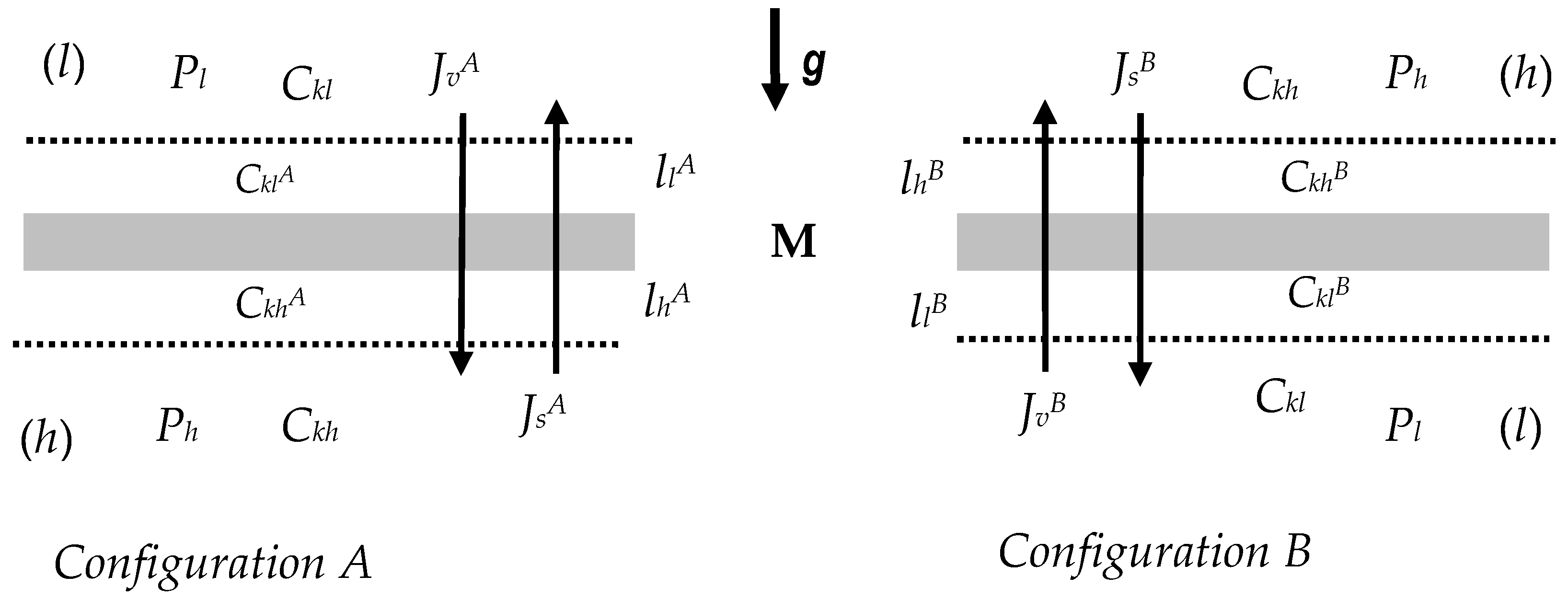
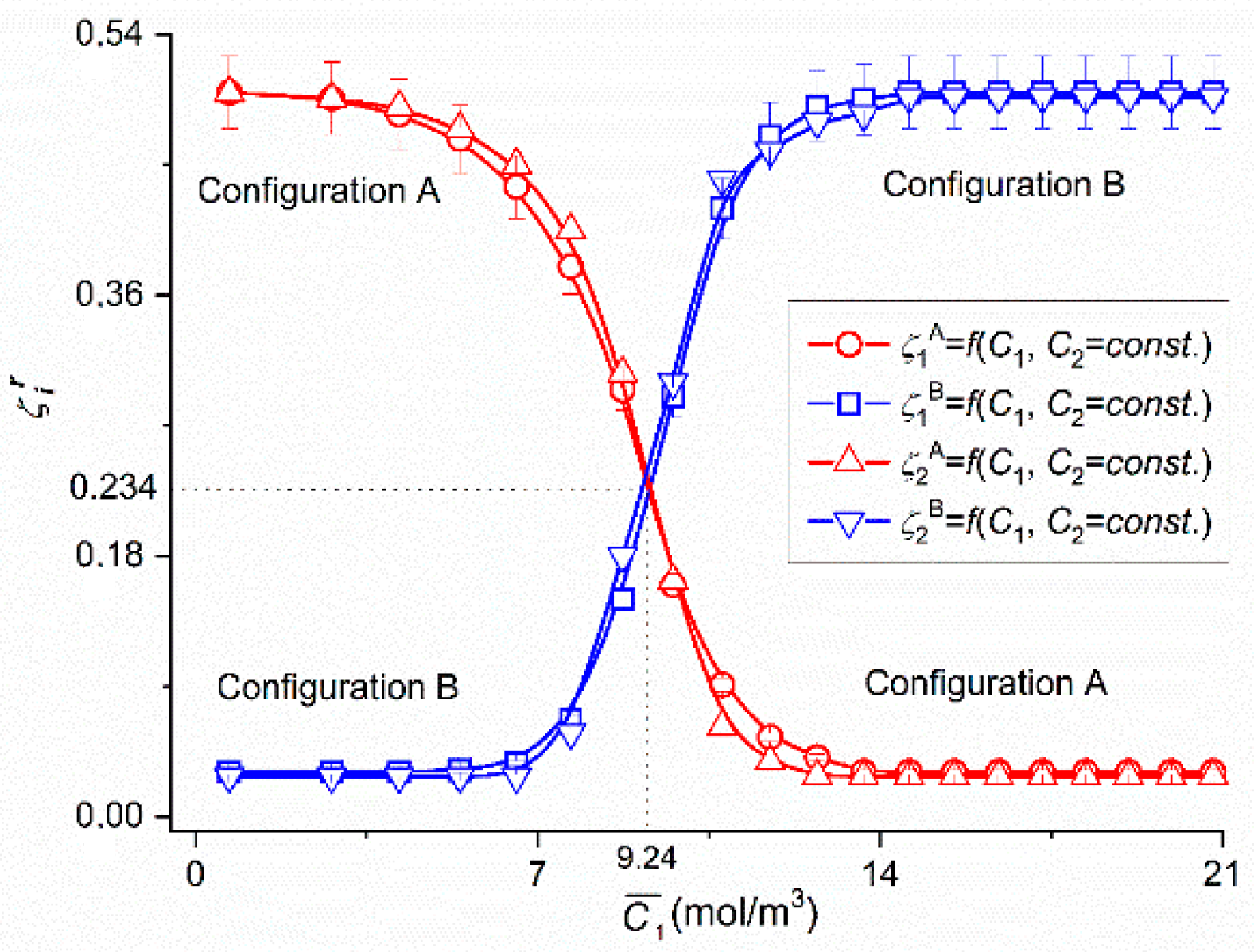
Figure 2. The points (○,△) were obtained for Configuration A and points (□,▽) for Configuration B of single-membrane system.
Figure 2 shows that in the case of Configuration A for 0 <
≤ 4 mol/m
3,
=
= 0.5 = constant and for 4 mol/m
3 <
≤ 12.72 mol/m
3 the values of coefficients
and
decrease nonlinearly and for
> 12.72 mol/m
3 reach constant value equal respectively to
=
= 0.03. In the case of Configuration B for 0 <
≤ 5.41 mol/m
3,
=
= 0.03 = constant, and for 5.41 mol/m
3 <
≤ 12.72 mol/m
3 the values of coefficients
and
increase and for
> 12.72 mol/m
3 reach constant value equal respectively to
=
= 0.5. The results presented in this figure show that 0.5 ≥
≥ 0.03 and 0.03 ≤
≤ 0.5. This notation indicates that for the same values
and
the value of coefficient
decreases from 0.5 to 0.03 and coefficient
increases from 0.03 to 0.5.
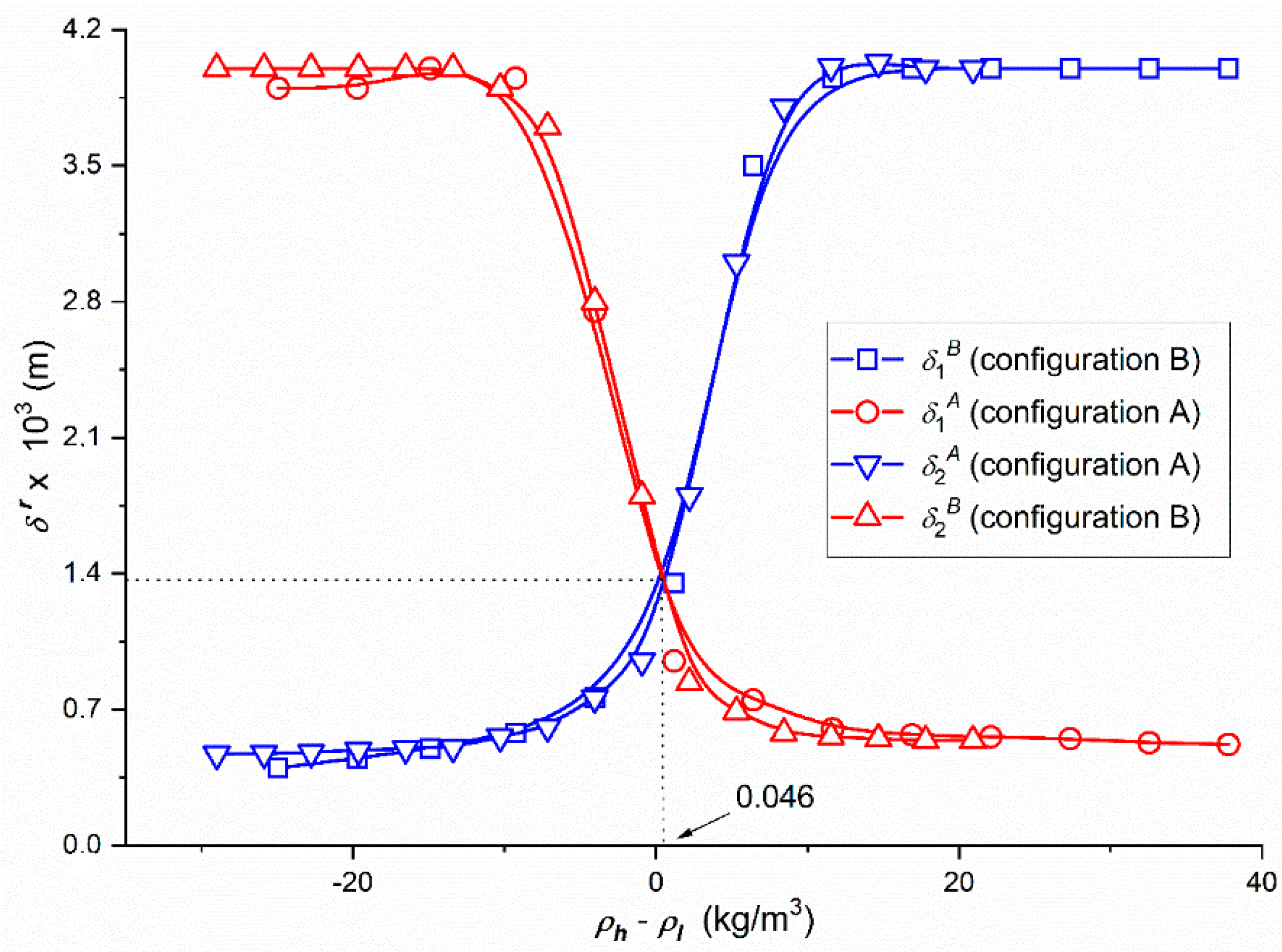
Figure 3 shows that in Configuration A for −30 kg/m
−3 <
≤ −8.5 kg/m
−3,
= 3.95 × 10
−3 m = constant and for −8.5 kg/m
−3 <
≤ 7.9 kg/m
−3 the values of coefficients
decrease nonlinearly and for
> 7.9 kg/m
−3 reach constant value equal respectively to
= 0.52 × 10
−3 m = constant. For −30 kg/m
−3 <
≤ −8.5 kg/m
−3,
= 0.52 × 10
−3 m = constant and for –8.5 kg/m
–3 <
≤ 7.9 kg/m
−3 the values of coefficients
decrease nonlinearly and for
> 7.9 kg/m
−3 reach constant value equal respectively to
= 3.95 × 10
−3 m = const. The results presented in
Figure 3 show that 3.95 × 10
−3 m ≥
≥ 0.52 × 10
−3 m and 0.52 × 10
−3 m ≤
≤ 3.95 × 10
−3 m. This notation indicates that for the same values
the value of coefficient
decreases from 3.95 × 10
−3 m to 0.52 × 10
−3 m and coefficient
increases from 0.52 × 10
−3 m to 3.95 × 10
−3 m.
In addition, it can be seen from the
Figure 2 and
Figure 3 that for
< 9.24 mol/m
3 and
≤ 0.046 kg/m
−3 in Configuration A, the complex of CBLs is hydrodynamically unstable and in Configuration B—hydrodynamically stable, because the solutions of ethanol prevailing over glucose are under the membrane, and for that case the solution density under the membrane is lower than the solution density over the membrane. In Configuration B, the complex of CBLs is stable because density of the solution under the membrane is greater than the solution above the membrane. In turn for
> 9.24 mol/m
3 and
> 0.046 kg/m
−3 in Configuration A, the complex of CBLs is hydrodynamically stable, and in Configuration B—hydrodynamically unstable due to the fact that in solutions separated by the membrane, glucose concentration is greater than ethanol and density of solution under the membrane is greater than the solution over the membrane. In Configuration B, the complex of CBLs is unstable because density of the solution under the membrane is smaller than the solution above the membrane. This causes the convection movements vertically downward. For
= 9.24 mol/m
3 and
= 0.046 kg/m
−3 the CBL
S complex is independent of the membrane system configuration and therefore
=
= 0.234 and
=
= 1.3 × 10
−3 m. In Configuration A, a non-convective state occurs, when the density of the solution in the compartment above the membrane is higher than density of the solution in the compartment under the membrane. In Configuration A natural convection occurs when
ρl >
,
>
ρh and
>
and is directed vertically upwards. On the other hand, in Configuration B, a natural convection occurs when
ρl <
,
<
ρh and
<
and is directed vertically downwards [
38]. Natural convection allows it to increase the value fluxes of
and
.
3.2. Concentration Dependencies of Coefficients , , and
To calculate
,
,
and
, (
i,
j ∈ {1, 2, 3},
r = A, B), based on Equations (5)–(8) respectively, the characteristics
= 37.71 mol/m
3) and
= 37.71 mol/m
3) presented in
Figure 2 and following data:
Lp = 4.9 × 10
–12 m
3/Ns,
σ1 = 0.068,
σ2 = 0.025,
ω11 = 0.8 × 10
−9 mol/Ns,
ω12 = 0.81 × 10
−13 mol/Ns,
ω22 = 1.43 × 10
−9 mol/Ns,
ω21 = 1.63 × 10
−12 mol/Ns,
= 2.79 ÷ 21.67 mol/m
3 and
= 37.71 mol/m
3 were used. The results of calculating these coefficients are presented in
Figure 4,
Figure 5,
Figure 6,
Figure 7,
Figure 8,
Figure 9 and
Figure 10.
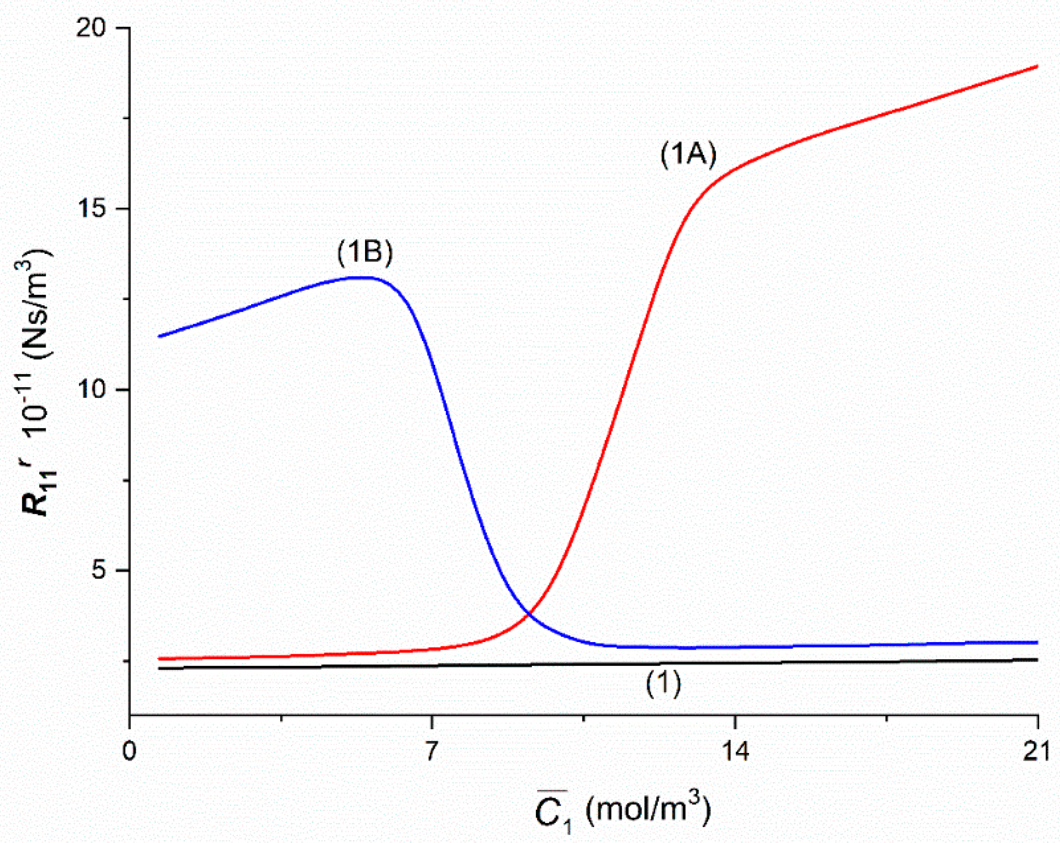
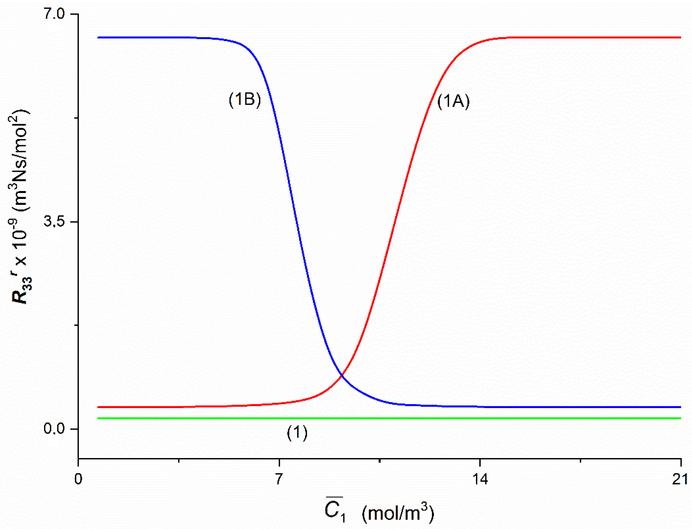
The Graphs 1A and 1B in
Figure 4 illustrating the dependencies
=
f(
,
= 37.71 mol/m
3) and
=
f(
,
= 37.71 mol/m
3) were obtained for the Configurations A and B of the membrane system. The value of coefficient
increases initially nonlinearly from
= 2.57 × 10
11 Ns/m
3 (for
= 1.44 mol/m
3) to
= 2.89 × 10
11 Ns/m
3 (for
= 7.56 mol/m
3) and next increases nonlinearly to
= 16.45 × 10
11 Ns/m
3 (for
= 14.59 mol/m
3). For
> 16.45 mol/m
3 increases approximately linearly and for
= 21.67 mol/m
3 and
= 37.71 mol/m
3 achieves the value
= 19.2 × 10
11 Ns/m
3. The value of coefficient
initially increases linearly from
= 11.47 × 10
11 Ns/m
3 (for
= 1.44 mol/m
3) to
= 13.22 × 10
11 Ns/m
3 (for
= 5.41 mol/m
3) and next decreases almost linearly from
= 12.86 × 10
11 Ns/m
3 (for
= 6.57 mol/m
3) to
= 4.14 × 10
11 Ns/m
3 (for
= 8.74 mol/m
3). Besides
R11A=
= 3.67 × 10
11 Ns/m
3 (for
= 9.24 mol/m
3). For
> 12.72 mol/m
3 increases approximately linearly and for
= 21.67 mol/m
3 achieves the value
= 3.04 × 10
11 Ns/m
3. For homogeneous solutions
=
=
R11 increase linearly from
R11 = 2.3 × 10
11 Ns/m
3 (for
= 1.44 mol/m
3) to
R11 = 2.53 × 10
11 Ns/m
3 (for
= 21.67 mol/m
3). Besides, it follows from this figure that for
< 9.24 mol/m
3 <
and for
> 9.24 mol/m
3 >
.
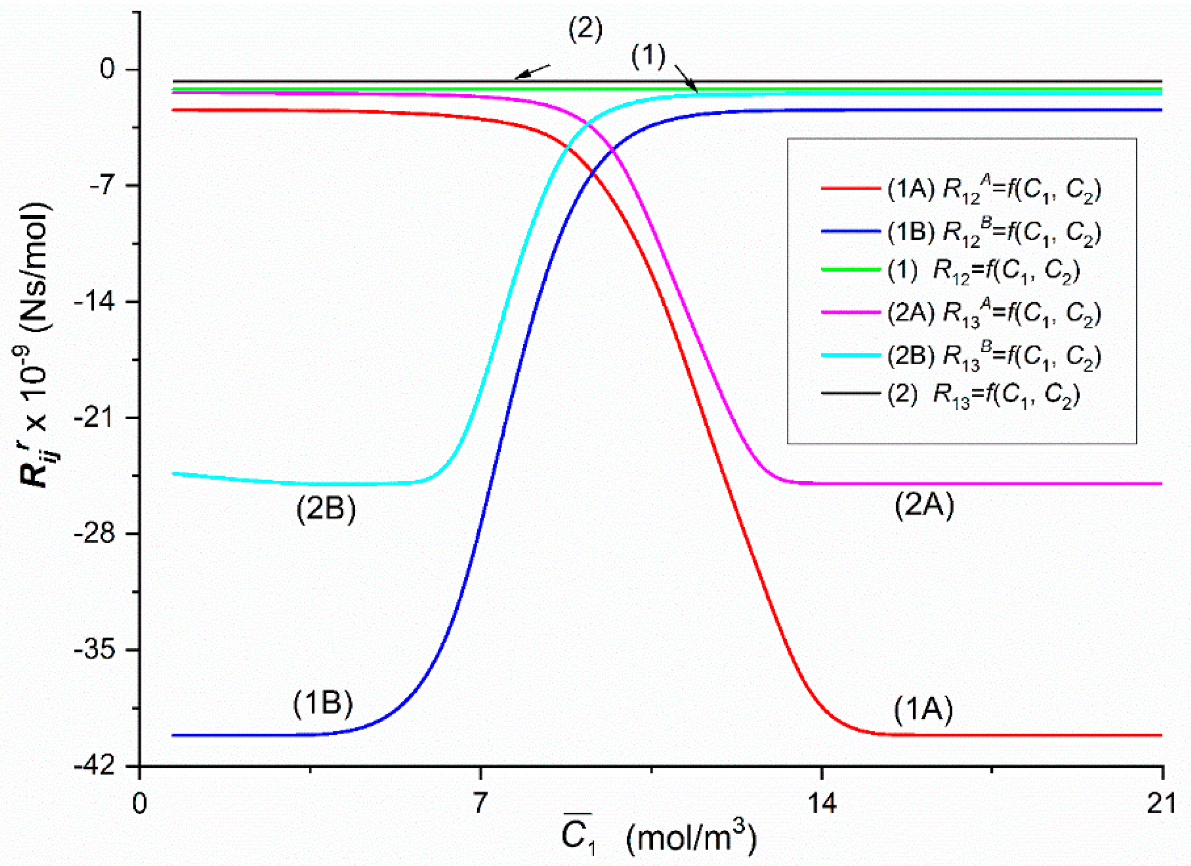
The Graphs 1A, 1B, 2A and 2B illustrating dependencies
=
f(
,
= 37.71 mol/m
3),
=
f(
,
= 37.71 mol/m
3),
=
f(
,
= 37.71 mol/m
3) and
=
f(
,
= 37.71 mol/m
3) presented in
Figure 5, were obtained suitably for Configurations A and B of the membrane system, respectively. In the case of Configuration A, the value of coefficients
and
decreases nonlinearly from
= −2.41 × 10
9 Ns/mol and
= −1.41 × 10
9 Ns/mol (for
= 5.41 mol/m
3) to
= −39.95 × 10
−9 Ns/mol (for
= 14.59 mol/m
3) and to
= −24.76 × 10
9 Ns/mol (for
= 13.66 mol/m
3).
(for
≥ 15.51 mol/m
3) and
(for
≥ 12.72 mol/m
3) are constant and amounts to
= −40.15 × 10
9 Ns/mol and
= −24.95 × 10
9 Ns/mol, respectively. The value of coefficients
and
increases nonlinearly from
= −40.15 × 10
9 Ns/mol and
= −24.34 × 10
−9 Ns/mol (for
= 0.69 mol/m
3) to
= −2.46 × 10
9 Ns/mol and
=
= −1.43 × 10
9 Ns/mol (for
= 12.72 mol/m
3). For
> 13.66 mol/m
3,
and
are constant and amounts to
= −2.41 × 10
−9 Ns/mol and
= −1.39 × 10
9 Ns/mol. For
= 9.24 mol/m
3 and
= 37.71 mol/m
3 =
= −6.0 × 10
9 Ns/mol and
=
= −3.0 × 10
9 Ns/mol. Besides, for
< 9.24 mol/m
3 >
and
>
. For
> 9.24 mol/m
3 <
and
<
. For homogeneous solutions
=
=
R12 = −1.16 × 10
9 Ns/mol <
=
=
R13 = −0.68 × 10
9 Ns/mol in whole range of studied
(Lines 1 and 2).
The Graphs 1A, 1B, 2A and 2B present dependencies
=
f(
,
= 37.71 mol/m
3),
=
f(
,
= 37.71 mol/m
3),
=
f(
,
= 37.71 mol/m
3) and
=
f(
,
= 37.71 mol/m
3) presented in
Figure 5, were obtained suitably for Configurations A and B of the membrane system, respectively. In the case of Configuration A, the value of coefficients
and
decreases nonlinearly from
= −2.41 × 10
9 Ns/mol and
= −1.41 × 10
9 Ns/mol (for
= 5.41 mol/m
3) to
= −39.95 × 10
−9 Ns/mol (for
= 14.59 mol/m
3) and to
= −24.76 × 10
9 Ns/mol (for
= 13.66 mol/m
3).
(for
≥ 15.51 mol/m
3) and
(for
≥ 12.72 mol/m
3) are constant and amounts to
= −40.15 × 10
9 Ns/mol and
= −24.95 × 10
9 Ns/mol, respectively. The value of coefficients
and
increases nonlinearly from
= −40.15 × 10
9 Ns/mol and
= −24.34 × 10
−9 Ns/mol (for
= 0.69 mol/m
3) to
= −2.46 × 10
9 Ns/mol and
=
= −1.43 × 10
9 Ns/mol (for
= 12.72 mol/m
3). For
> 13.66 mol/m
3,
and
are constant and amounts to
= −2.41 × 10
−9 Ns/mol and
= −1.39 × 10
9 Ns/mol. For
= 9.24 mol/m
3 and
= 37.71 mol/m
3 =
= −6.0 × 10
9 Ns/mol and
=
= −3.0 × 10
9 Ns/mol. Besides, for
< 9.24 mol/m
3 >
and
>
. For
> 9.24 mol/m
3 <
and
<
. For homogeneous solutions
=
=
R12 = −1.16 × 10
9 Ns/mol <
=
=
R13 = −0.68 × 10
9 Ns/mol in whole range of studied
(Lines 1 and 2).
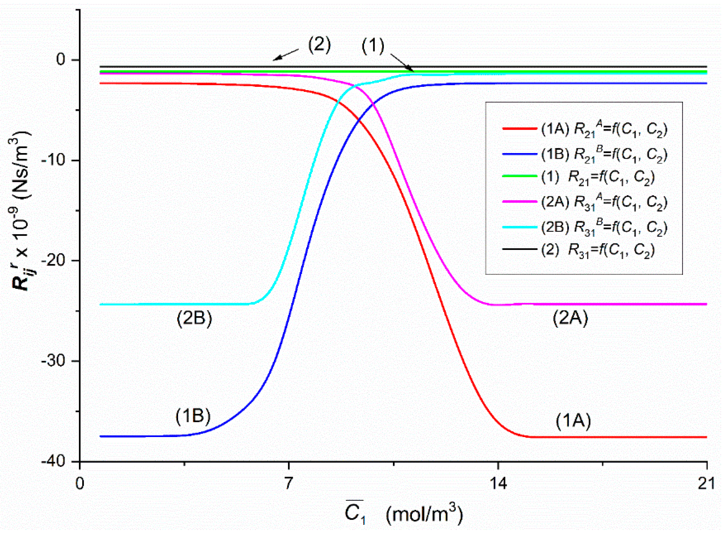
Graphs 1A, 1B, 2A and 2B illustrating dependencies
=
f(
,
= 37.71 mol/m
3),
=
f(
,
= 37.71 mol/m
3),
=
f(
,
= 37.71 mol/m
3) and
=
f(
,
= 37.71 mol/m
3), presented in
Figure 6, were obtained suitably for Configurations A and B of the membrane system, respectively. The dependencies shown in this figure are similar to the dependencies shown in
Figure 5.
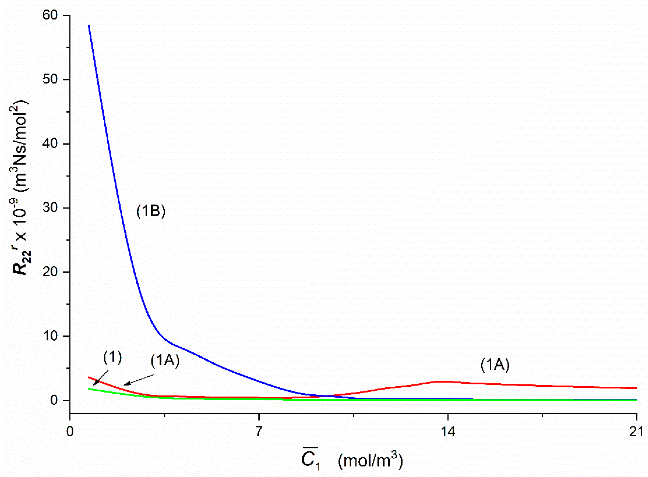
The Graphs 1A and 1B, illustrating the dependencies
=
f(
,
= 37.71 mol/m
3) and
=
f(
,
= 37.71 mol/m
3), presented in
Figure 7, were obtained for the Configurations A and B of the membrane system. Curves 1 and 1B illustrate the dependencies
R22 =
f(
,
= 37.71 mol/m
3) and
=
f(
,
= 37.71 mol/m
3) are hyperbolas. In turn, Curve 1A, illustrating the dependence
=
f(
,
), is an irregular curve: initially it decreases nonlinearly from
= 3.62 × 10
9 m
3Ns/mol
2 (for
= 1.44 mol/m
3) to
= 0.43 × 10
9 m
3Ns/mol
2 (for
= 7.68 mol/m
3) and then grows nonlinearly to
= 2.95 × 10
9 m
3Ns/mol
2 (for
= 13.66 mol/m
3). For
> 13.66 mol/m
3 decreases linearly to
= 1.86 × 10
9 m
3Ns/mol
2 (for
= 21.67 mol/m
3). In turn for
= 9.24 mol/m
3 =
= 0.64 × 10
9 m
3Ns/mol
2, while for
< 9.24 mol/m
3 <
and for
> 9.24 mol/m
3 >
.
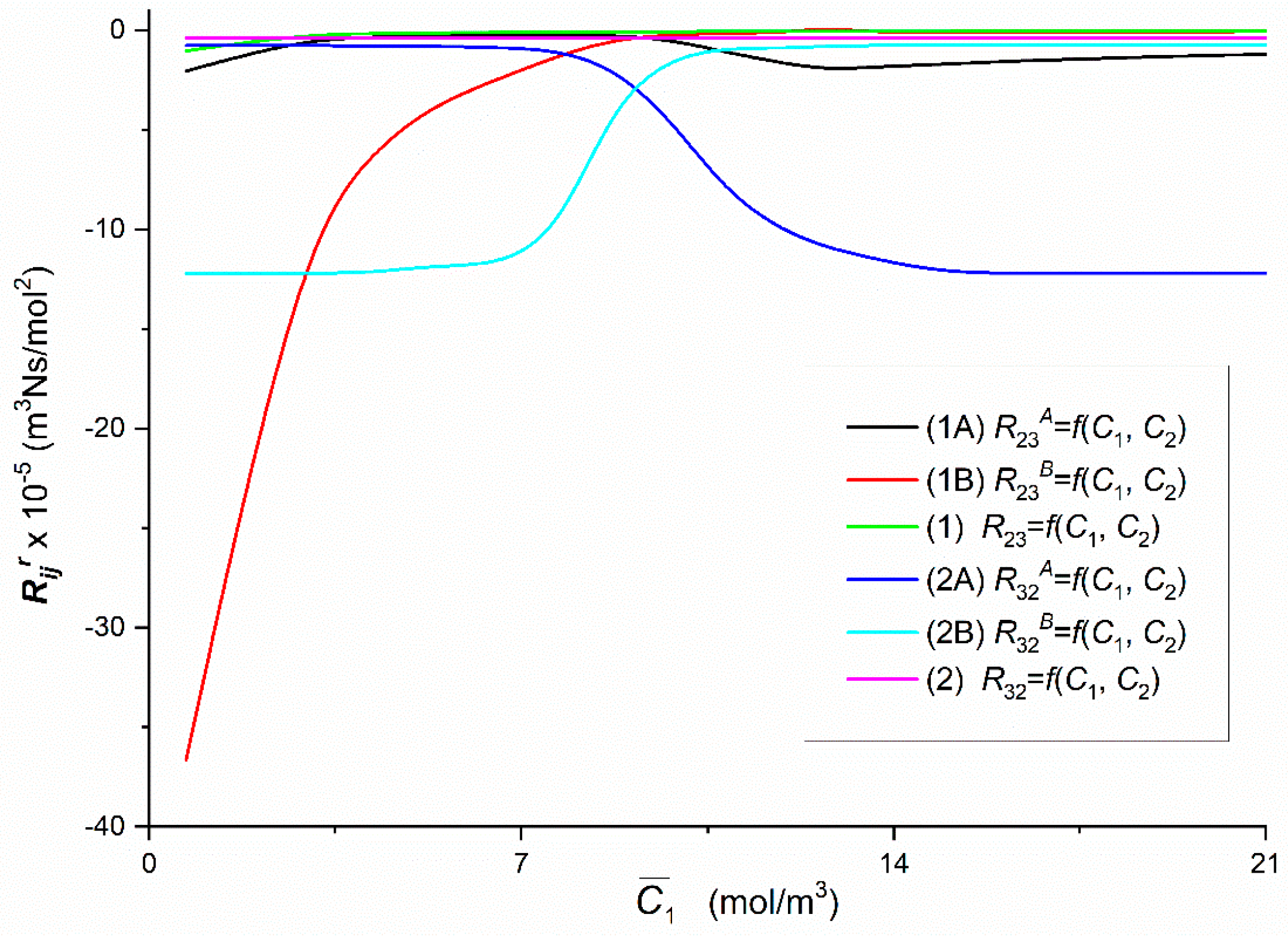
Graphs 1A, 1B, 2A and 2B illustrate dependencies
=
f(
,
= 37.71 mol/m
3 = const.),
=
f(
,
= 37.71 mol/m
3 = const.),
=
f(
,
= 37.71 mol/m
3 = const.) and
=
f(
,
= 7.71 mol/m
3 = const.) as presented in
Figure 8, were obtained suitably for Configurations A and B of the membrane system, respectively. Curves 1, 2 and 1B illustrate dependencies
R23 =
f(
,
= 37.71 mol/m
3 = const.),
R32 =
f(
,
= 37.71 mol/m
3 = const.) and
=
f(
,
= 37.71 mol/m
3 = const.) are hyperbolas. In turn, Curve 1A illustrating the dependence
=
f(
,
= 37.71 mol/m
3 = const.) is an irregular curve: initially it grows nonlinearly from
= −2.05 × 10
5 m
3Ns/mol
2 (for
= 1.44 mol/m
3) to
= −0.23 × 10
5 m
3Ns/mol
2 (for
= 7.68 mol/m
3) and then decreases nonlinearly to
= −1.99 × 10
5 m
3Ns/mol
2 (for
= 13.66 mol/m
3). For
> 12.71 mol/m
3 increases linearly to
= −1.17 × 10
5 m
3Ns/mol
2 (for
= 21.67 mol/m
3). For
= 9.24 mol/m
3,
=
= −0.38 × 10
5 m
3Ns/mol
2, while for
< 9.24 mol/m
3 >
and for
> 9.24 mol/m
3 <
Curves 2A and 2B illustrating respectively the dependence
=
f(
,
) and
R32B=
f(
,
) intersect at the coordinates
= 9.24 mol/m
3 and
=
= −2.66 × 10
5 m
3Ns/mol
2. For
< 9.24 mol/m
3 >
and for
> 9.24 mol/m
3 <
.
Presented in
Figure 9, Graphs 1A and 1B illustrating the dependencies
=
f(
,
= 37.71 mol/m
3) and
=
f(
,
= 37.71 mol/m
3) were obtained for Configurations A and B of the membrane system. The value of coefficient
increases nonlinearly from
= 0.37 × 10
9 m
3Ns/mol
2 (for
= 1.44 mol/m
3) to
= 6.51 × 10
9 m
3Ns/mol
2 (for
= 13.66 mol/m
3). For
> 13.66 mol/m
3 = 6.61 × 10
9 m
3Ns/mol
2 and is constant. The value of coefficient
in Configuration B of the membrane system initially is constant and for
> 1.44 mol/m
3 increases nonlinearly from
= 6.61 × 10
9 m
3Ns/mol
2 (for
= 0.69 mol/m
3) to
= 0.38 × 10
9 m
3Ns/mol
2 (for
= 13.66 mol/m
3) and next achieves constant value
= 0.37 × 10
9 m
3Ns/mol
2 (for
> 13.66 mol/m
3). Besides
=
= 0.82 × 10
9 m
3Ns/mol
2 for
= 9.24 mol/m
3 and
= 37.71 mol/m
3. For homogeneous solutions
=
=
R33,
R33 = 0.18 × 10
9 m
3Ns/mol
2 (for
= 0.69 mol/m
3). Besides, it follows from this figure that for
< 9.24 mol/m
3 <
and for
> 9.24 mol/m
3 >
.
The curves presented in
Figure 2,
Figure 3,
Figure 4,
Figure 5,
Figure 6,
Figure 7,
Figure 8 and
Figure 9, marked with a number and letters A or B, show that there are transition points from a linear wave to a non-linear wave or vice versa. It is related to the change of the nature of membrane transport from osmotic-diffusion to osmotic-diffusion-convective, or—inversely. The mechanism of this process is as follows. As the concentration of glucose increases at a given concentration of ethanol, the density of the solution, filling the compartment under the membrane in Configuration B, increases. If the density of this solution is lower than the density of the solution filling the compartment above the membrane, natural convection occurs in Configuration B, which causes destruction of CBLs, increasing driving forces and increasing the value of the coefficient. The addition of glucose stabilizes the layers and finally eliminates natural convection and changes the nature of transport from osmotic-diffusion-convective to osmotic-diffusion. In Configuration A, the process of creating gravitational convection is in the reverse order. This means that in Configuration A we have a transition from non-convective to convective, and in Configuration B—from convective to non-convective states. These transitions have a pseudo-phase transition character.
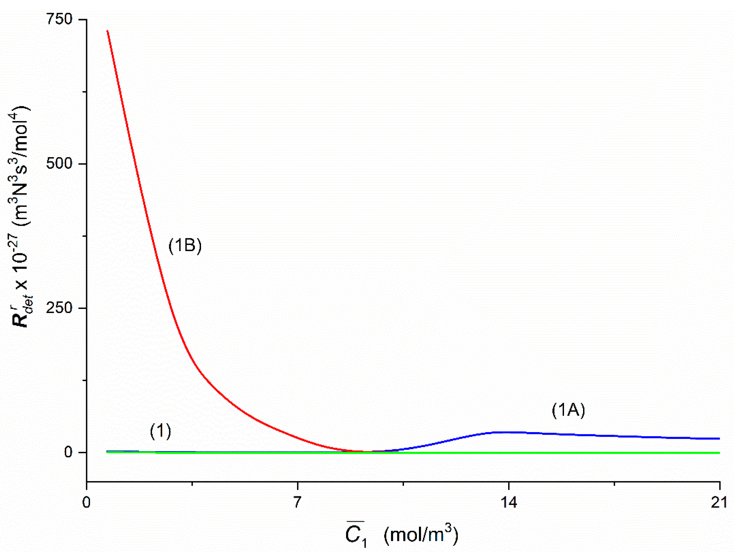
To calculate coefficients
and
the Equations (6) and (8) were used, respectively. The Graphs 1A and 1B presented in
Figure 10 and illustrating the dependencies
=
f(
,
= 37.71 mol/m
3 = const.) and
=
f(
,
= 37.71 mol/m
3 = const.) were obtained for the Configurations A and B of the membrane system. Curve 1B is hyperbolic. In turn, Curve 1A is an irregular curve: initially it decreases nonlinearly from
= 2.53 × 10
27 m
3N
3s
3/mol
4 (for
= 1.44 mol/m
3) to
= 0.7 × 10
27 m
3N
3s
3/mol
4 (for
= 7.68 mol/m
3) and then grows nonlinearly to
= 36.86 × 10
27 m
3N
3s
3/mol
4 (for
= 13.66 mol m
−3,
= 37.71 mol/m
3). For
> 13.66 mol/m
3 decreases linearly to the value of
= 23.24 × 10
27 m
3N
3s
3/mol
4 (for
= 21.67 mol/m
3). In turn for
= 9.24 mol/m
3 =
= 11.20 × 10
27 m
3N
3s
3/mol
4, whereas for
< 9.24 mol/m
3 <
and for
> 9.24 mol/m
3 >
. For homogeneous solutions,
=
=
increase linearly from
= 0.63 × 10
27 m
3N
3s
3/mol
4 (for
= 1.44 mol/m
3) to
= 0.02 × 10
27 m
3N
3s
3/mol
4 (for
= 21.67 mol/m
3).
3.3. Concentration Dependencies of and
To calculate coefficients
= (
−
)/
and
= (
det [
] –
det [
])/
det [
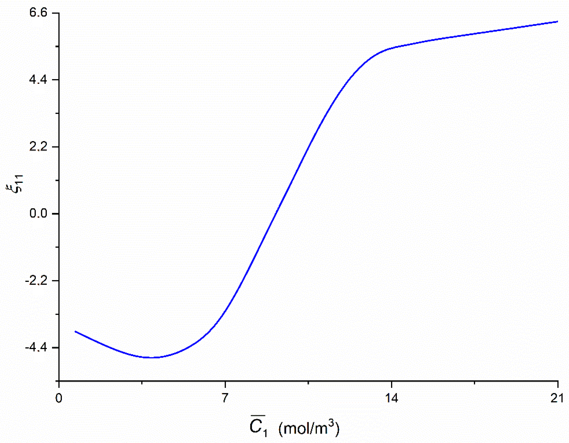
R] the Equations (9) and (10) were used, respectively. The graph presented in
Figure 11 illustrating the dependencies
=
f(
,
= 37.71 mol/m
3) was calculated on the basis of Equation (9). In that case the value of coefficient
initially decreases to
= −4.8 (for
= 1.44 mol/m
3) and next increases nonlinearly to
= 5.41 (for
= 13.66 mol/m
3) and then increases linearly to
= 6.39 (for
= 21.67 mol/m
3). Besides, it follows from this figure that for
= 9.24 mol/m
3 = 0 and that
< 9.24 mol/m
3 < 0 and for
> 9.24 mol/m
3 < 0.
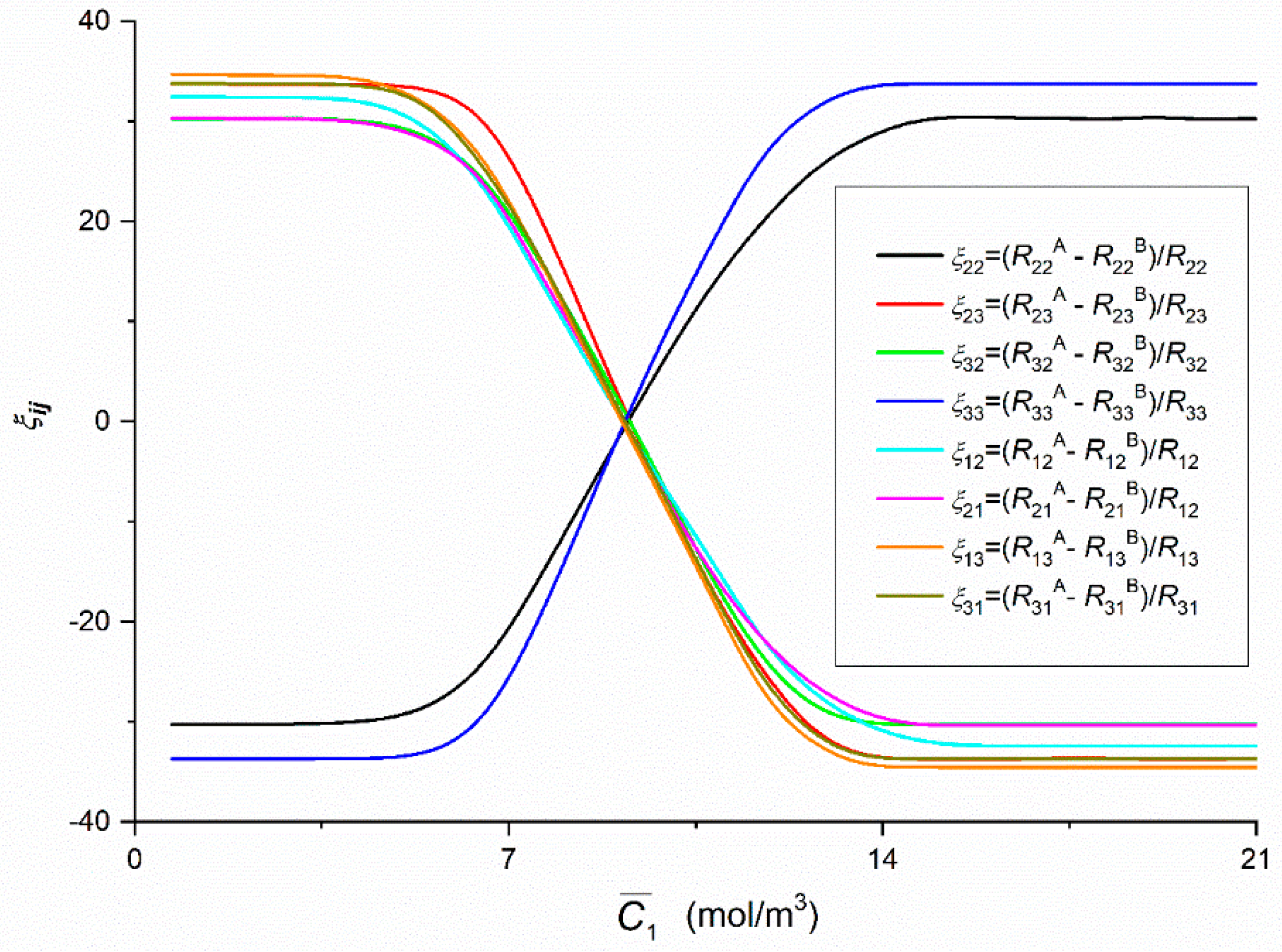
The graphs presented in
Figure 12 which illustrate the dependencies
ξ12 =
f(
,
= 37.71 mol/m
3),
ξ13 =
f(
,
= 37.71 mol/m
3),
ξ21 =
f(
,
= 37.71 mol/m
3),
ξ31 =
f(
,
= 37.71 mol/m
3),
ξ22 =
f(
,
= 37.71 mol/m
3),
ξ32 =
f(
,
= 37.71 mol/m
3),
ξ23 =
f(
,
= 37.71 mol/m
3) and
ξ33 =
f(
,
= 37.71 mol/m
3) were calculated on the basis of Equation (9). For these graphs, the value of coefficients
ξ12,
ξ13,
ξ21,
ξ31,
ξ23 and
ξ32 decreases nonlinearly (initially slowly and then faster) from
ξ12 > 0 = constant,
ξ13 > 0 = constant,
ξ21 > 0 = constant,
ξ31 > 0 = constant,
ξ23 > 0 = constant and
ξ32 > 0 = constant (
ξ21 <
ξ12 <
ξ31 <
ξ13 <
ξ32 <
ξ23), next
ξ12,
ξ13,
ξ21,
ξ31,
ξ23 and
ξ32 decreases linearly to
ξ12 < 0 = const.,
ξ13 < 0 = const,
ξ21 < 0 = const.,
ξ31 < 0 = const.,
ξ23 < 0 = const. and
ξ32 < 0 = constant (
ξ21 >
ξ32 >
ξ12 >
ξ23 >
ξ31 >
ξ13). It results from this figure that
ξ12 =
ξ13 =
ξ21 =
ξ31 =
ξ23 =
ξ32 = 0 for
= 9.24 mol/m
3. For these graphs the value of coefficients
ξ22 and
ξ33 increases nonlinearly (initially slowly and then faster) from
ξ22 < 0 = constant and
ξ33 < 0 = constant (
ξ22 >
ξ33), next
ξ22 and
ξ33 increases linearly to
ξ22 > 0 = const. and
ξ33 > 0 = constant. Besides, it follows from this figure that for
= 9.24 mol m
−3,
ξ22 =
ξ33 = 0.
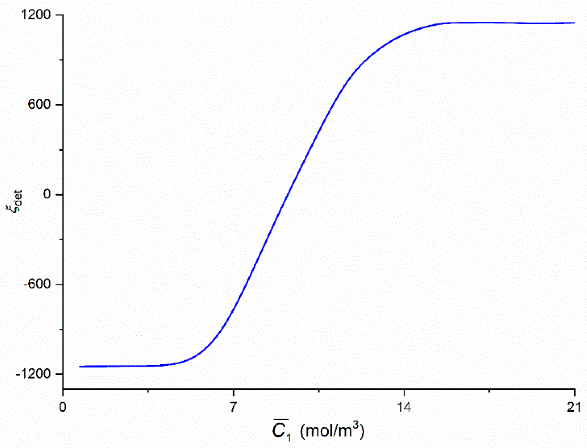
The graph presented in
Figure 13 illustrating the dependencies
ξdet =
f(
,
= 37.71 mol/m
3 = const.) was calculated on the basis of Equation (10). In the case of this curve the value of coefficient
ξdet initially is constant and amounts
ξdet = −0.034 and next increases nonlinearly to
ξdet = −1148.94 (for
= 1.44 mol/m
3), then increases linearly to
ξdet = 866.38 (for
= 12.73 mol/m
3) and next, nonlinearly to
ξdet = 1148.38 (for
≥ 21.67 mol/m
3). Besides, it follows from this figure that for
= 9.24 mol/m
3,
ξdet = 0.
In all cases of the dependencies,
=
f(
,
= 37.71 mol/m
3) (
i,
j ∈ {1, 2, 3},
r = A or B) and
=
f(
,
= 37.71 mol/m
3), (
r = A or B) shown in
Figure 5,
Figure 6,
Figure 7,
Figure 8,
Figure 9 and
Figure 10 show clearly that their values are determined by the hydrodynamic conditions in solutions near membrane which separates ternary non-electrolytes with different concentrations. It means that values of these coefficients in concentration polarization conditions are strongly connected with concentrations
and
and configuration of the membrane system. In turn, in the case of mechanical stirring of solutions, the values of these coefficients depend only on concentrations
and
. Therefore, for interpretation of calculation results, the combinations of coefficients
,
and
Rij (
i,
j ∈ {1, 2, 3) of the same indicators and
,
and
were used. These combinations are presented by Equations (5)–(10). Concentration dependencies of new coefficients facilitate the location of areas differentiated by hydrodynamic conditions in adjacent membrane areas such as diffusion, natural convection-diffusion and natural convection.
From the results presented in
Figure 4,
Figure 5,
Figure 6,
Figure 7,
Figure 8,
Figure 9 and
Figure 10, it also appears that the
and
(
i,
j ∈ {1, 2, 3},
r = A, B), have different physical significance. The unit of coefficients
,
and
is Ns/m
3. Therefore, they have the character of flow resistance coefficients (hydraulic resistance). In turn, the unit of coefficients
i
is Ns/mol, what makes them coefficients of flow resistance of dissolved substances (diffusion resistance). The unit of coefficients
,
,
and
is m
3Ns/mol
2. This unit is a measure of the ratio of diffusion resistance to concentration. The unit of the coefficient
is m
3N
3s
3/mol
4. It corresponds to the ratio of diffusion resistance raised to the power of third and concentration.
3.4. Concentration Dependencies of , , , , and
Figure 14,
Figure 15 and
Figure 16 show the dependences
=
f(
,
= 37.71 mol/m
3) and
=
f(
,
= 37.71 mol/m
3), (
i,
j ∈ {1, 2, 3} and
r = A, B) calculated on the basis of Equations (11) and (12) and data presented in
Figure 4,
Figure 5,
Figure 6,
Figure 7,
Figure 8 and
Figure 9.
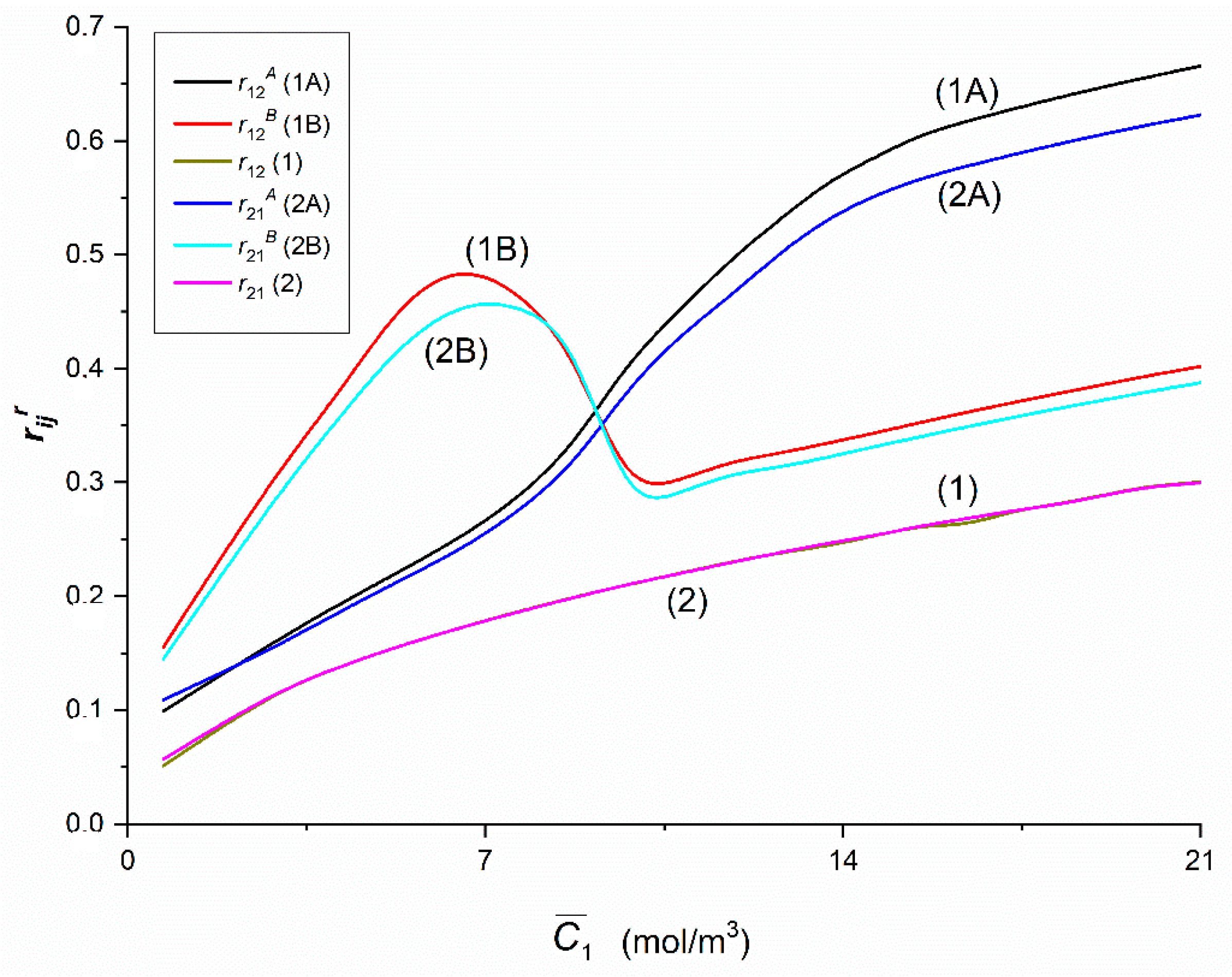
Figure 14 shows that Curves 1A and 1B intersect at a point with coordinates:
=
= 0.36 and
= 9.15 mol/m
3, and the Curves 2A and 2B—at a point with coordinates:
=
= 0.35 and
= 9.33 mol/m
3. The course of Curves 1A, 1B and 1 shows that for
< 9.15 mol/m
3,
>
>
and for
> 9.15 mol/m
3,
>
>
. Similarly, Curves 2A, 2B and 2 show that for
< 9.33 mol/m
3, >
>
and for
> 9.33 mol/m
3,
>
>
. Curves 1B and 2B have maxima. The coordinates of the maximum of Curve 1B are
= 0.48 and
= 6.53 mol/m
3. In turn, the coordinates of maximum of the 2B curve are
= 0.46 and
= 7.14 mol/m
3. This means that the maximum of Curve 1B is shifted relative to the maximum of Curve 2B vertically by (
−
) = 0.02 and horizontally by
= 0.61 mol/m
3. In addition, Curves 1A and 2A and Curves 1B and 2B are shifted relative to each other, except for the point with coordinates
=
= 0.14 and
= 2.15 mol/m
3. This means that for
< 2.15 mol/m
3 =
while for
> 2.15 mol/m
3 =
. Curves 1B and 2B coincide on the section with coordinates
=
= 0.48 and
= 8.03 mol/m
3 and
=
= 0.33 and
= 9.47 mol/m
3. For
< 8.03 mol/m
3 and
> 9.47 mol/m
3 the condition
>
is fulfilled. Curves 1 and 2 show that the condition
=
is fulfilled.
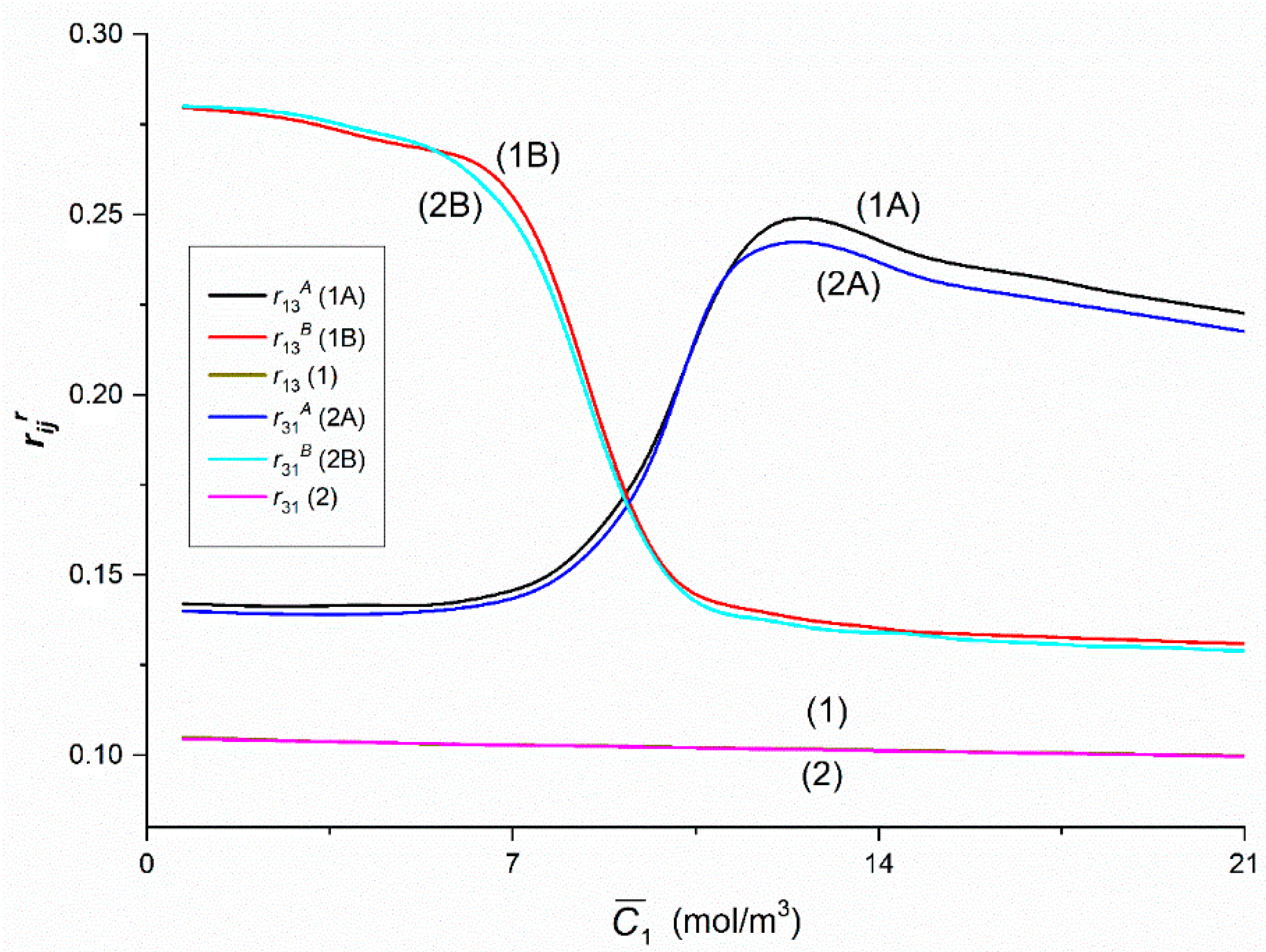
Figure 15 shows that Curves 1A and 1B intersect at a point with coordinates
=
= 0.17 and
= 9.1 mol/m
3, and Curves 2A and 2B—at a point with coordinates
=
= 0.17 i
= 9.29 mol/m
3. The course of Curves 1A, 1B and 1 shows that for
< 9.1 mol/m
3,
>
>
and for
> 9.1 mol/m
3,
>
>
. Similarly, Curves 2A, 2B and 2 show that for
< 9.29 mol/m
3,
>
>
and for
> 9.29 mol/m
3,
>
>
. Curves 1B and 2B overlap in the whole range of
used. Therefore, it can be assumed that
=
. In turn, Curves 1A and 2A do not coincide only beyond the point with the coordinates:
=
= 0.24 and
= 11.25 mol/m
3. For
> 11.25 mol/m
3,
>
. Curves 1 and 2 show that the condition
=
is fulfilled.
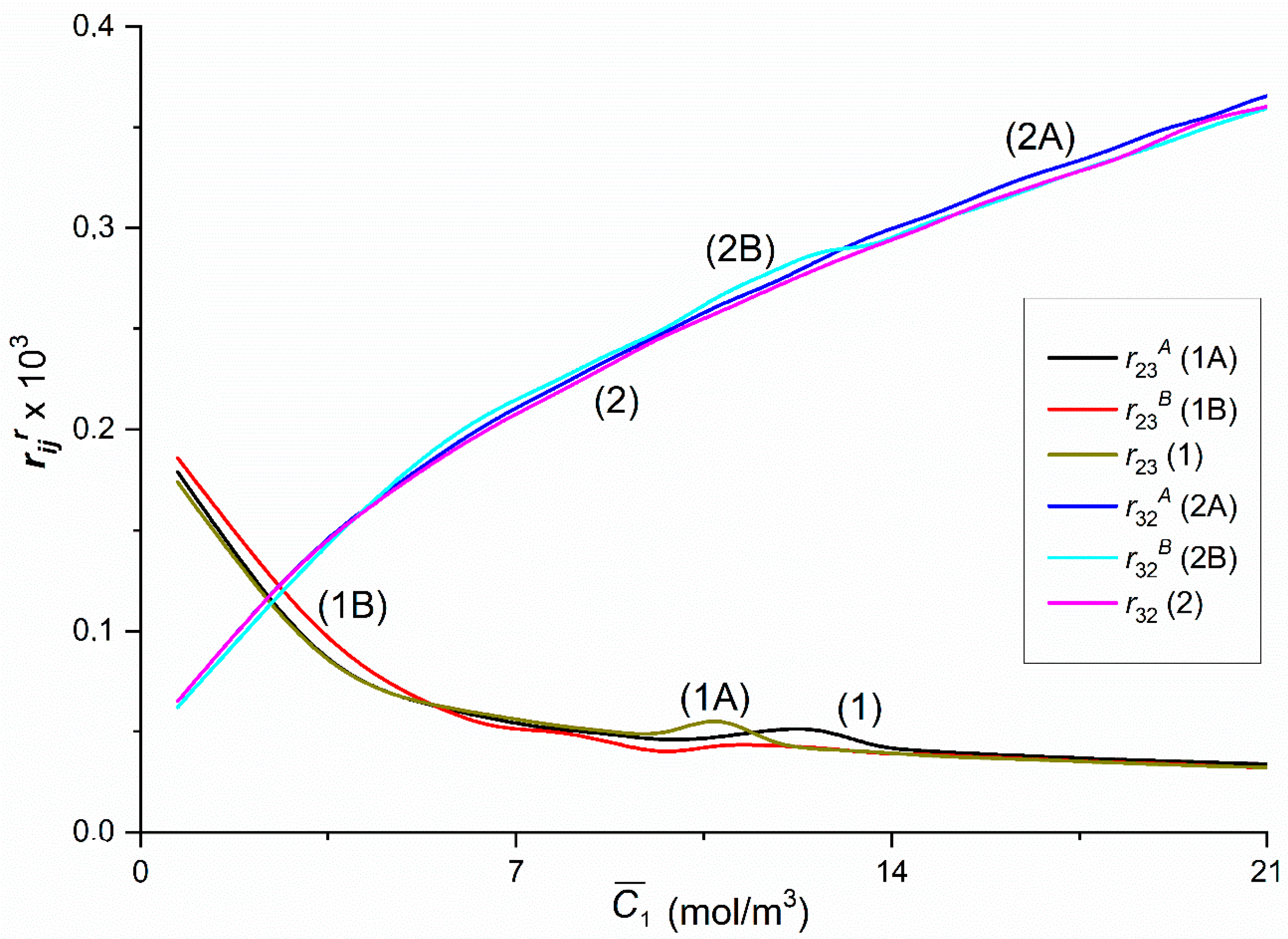
From the course of curves shown in
Figure 16, it follows that
=
=
and
=
=
. Curves 1 and 2 and 1A and 2B intersect at a point with coordinates
=
=
=
= 0.11 × 10
−3 and
= 2.33 mol/m
3, while Curves 1B and 2A—at a point with coordinates
=
= 0.12 and
= 2.6 mol/m
3. For
< 2.33 mol/m
3,
=
=
>
=
=
=
and for
> 2.33 mol/m
3,
=
=
>
=
=
. As can be seen, the values of the coefficients
,
,
and
(
i,
j ∈ {2, 3} and
r = A, B) (
Figure 16) are three orders of magnitude smaller than the values of the coefficients
,
,
and
(
i,
j ∈ {1, 2} and
r = A, B) and
,
,
and
(
i,
j ∈ {1, 3} and
r = A, B) (
Figure 14 and
Figure 15).
Figure 14,
Figure 15 and
Figure 16 show that Kedem–Caplan relations take the form: 0.05 ≤
=
≤ 0.3, 0.1 ≤
≤ 0.67, 0.15 ≤
≤ 0.48, 0.11 ≤
≤ 0.63, 0.15 ≤
≤ 0.46, 0.1 ≤
=
≤ 0.11, 0.14 ≤
≤ 0.24, 0.13 ≤
≤ 0.28, 0.11 ≤
≤ 0.24, 0.13 ≤
≤ 0.25, 0.03 × 10
−3 ≤
=
=
≤ 0.18 × 10
−3, 0.06 × 10
−3 ≤
=
=
≤ 0.36 × 10
−3. Hence it follows that,
≠
,
≠
,
≈
,
=
,
=
=
≠
=
=
. The values of all coupling coefficients presented in
Figure 8a,b and
Figure 9a fulfilled the conditions 0 ≤
≤ 1, 0 ≤
≤ 1, 0 ≤
≤ 1 and 0 ≤
≤ 1 determined by Roy Caplan [
20].
Graphs in
Figure 14 and
Figure 15 have characteristic shapes, depending on the configuration of the membrane system and the properties of the solutions. In the case of homogeneous solutions (mechanically stirred solutions—Graphs 1 and 2), the coefficients do not depend on the configuration of the membrane system and are approximately linearly dependent on the concentration of glucose. This means that mechanical stirring of solutions at a sufficiently high speed eliminates CBL creation and causes maximization of fluxes and forces on the membrane. In the case of heterogeneous solutions (without mechanical stirring of the solutions in the chambers), the appearance of CBL near the membrane, reduces the value of the respective fluxes and increases the value of coupling factors for the same concentrations of solute in relation to homogeneous conditions. In addition, coupling coefficients for heterogeneous conditions strongly depend on the membrane configuration.
In Configuration A, the increase in glucose at a constant ethanol concentration at the beginning causes an increase in the coupling coefficients. In Configuration B, an increase in glucose causes a decrease in the value of coupling coefficients. The range of glucose concentrations for which the change in coupling coefficients in Configuration B is maximum is within the range similar to Configuration A of the membrane system. Analyzing the characteristics of coupling coefficients in heterogeneous conditions, we observed that for the respective characteristics in the A and B configurations of the membrane system, the respective graphs pairs (1A and 1B, 2A and 2B) intersect at a concentration of about 9.2 mol m−3. At this glucose concentration, the densities of the ternary solutions in the upper and lower chambers at the initial moment are the same. In this case, we observed the appearance of hydrodynamic instabilities that cause a disturbance of CBL diffusion reconstruction. Despite the fact that the solution densities were the same at the initial moment, the diffusion of glucose and ethanol through the membrane caused the appearance of sufficiently large and concentration gradients (and density gradients) in opposite direction to the gravitational field in the CBL areas. These gradients can cause hydrodynamic instabilities in the membrane system.
Graphs in
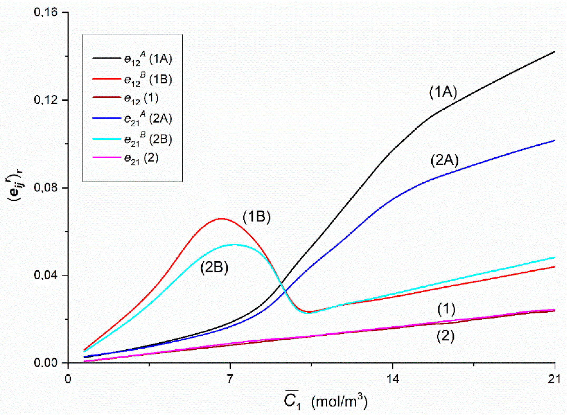
Figure 17 show that in the case of heterogeneous solutions (solutions not mechanically mixed—Graphs 1A and 1B, 2A and 2B), the coupling factors do not show their dependence on the configuration of the membrane system. Perhaps, because their value is very small.
Figure 17,
Figure 18 and
Figure 19 show the dependences
=
f(
,
= 37.71 mol/m
3) and
=
f(
,
= 37.71 mol/m
3), (
i,
j ∈ {1, 2, 3} and
r = A, B) calculated on the basis of Equations (13) and (14) and data presented in
Figure 14,
Figure 15 and
Figure 16.
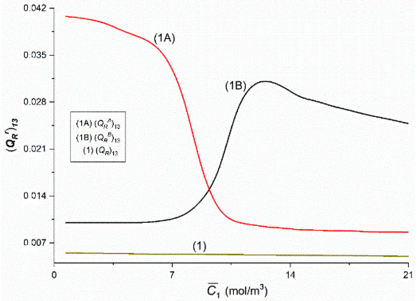
Figure 17 shows that Curves 1A and 1B intersect at a point with coordinates:
=
= 0.036 and
= 9.18 mol/m
3, and Curves 2A and 2B—at a point with coordinates:
=
= 0.032 and
= 9.41 mol/m
3. The course of Curves 1A, 1B and 1 shows that for
< 9.18 mol/m
3,
>
>
and for
> 9.18 mol/m
3,
>
>
. Similarly, the Curves 2A, 2B and 2 show that for
< 9.41 mol/m
3, >
>
and for
> 9.41 mol/m
3,
>
>
. Curves 1B and 2B have maxima. The coordinates of the maximum of Curve 1B are
= 0.065 and
= 6.54 mol/m
3. In turn, the coordinates of maximum of the 2B curve are
= 0.054 and
= 7.23 mol/m
3. This means that the maximum Curve 1B is shifted relative to the maximum Curve 2B vertically by (
−
) = 0.011 and horizontally by
= 0.69 mol/m
3. Curves 1B and 2B coincide on the section with coordinates:
=
= 0.045 and
= 8.73 mol/m
3 and
=
= 0.028 and
= 13.09 mol/m
3. For
< 8.73 mol/m
3 the conditions:
>
(for
> 13.09 mol/m
3) and
<
are fulfilled. Curves 1 and 2 show that the condition
=
is fulfilled.
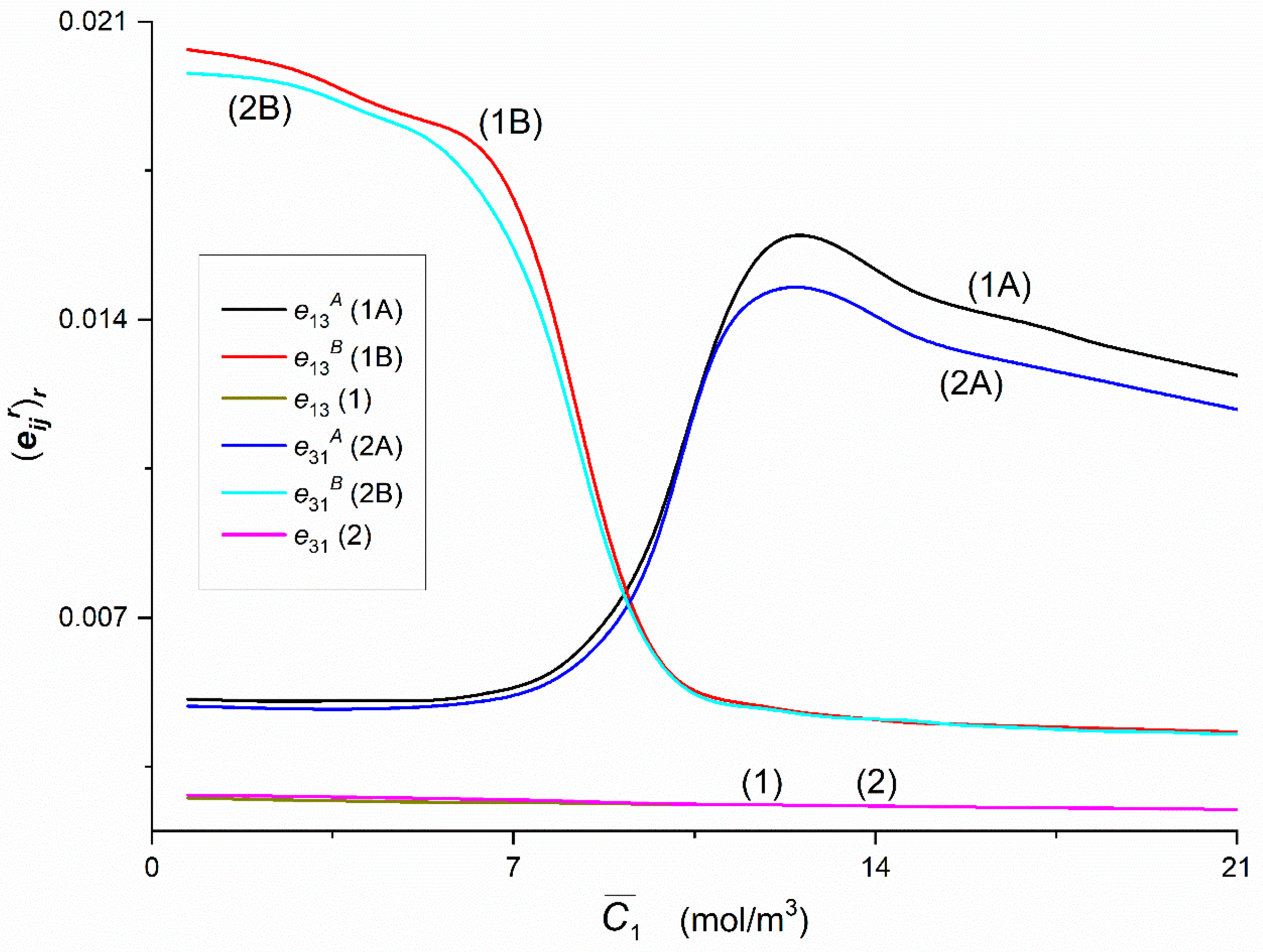
Figure 18 shows that Graphs 1A, 1B, 2A and 2B intersect approximately at the point with the coordinates
=
≈ 0.008 and
= 9.24 mol/m
3. Curves 1A, 1B and 1 show that for
< 9.24 mol/m
3 >
>
and for
> 9.24 mol/m
3 >
>
. Similarly, the course of Curves 2A, 2B and 2 shows that for
< 9.24 mol/m
3 >
>
and for
> 9.24 mol/m
3 >
>
. Curves 1B and 2B coincide for
> 9.24 mol/m
3. Therefore, it can be assumed that for this concentration range
>
>
. In the other ranges
Curves 1A and 2A do not cover. This means that
>
and
>
. Curves 1 and 2 show that the condition
=
.
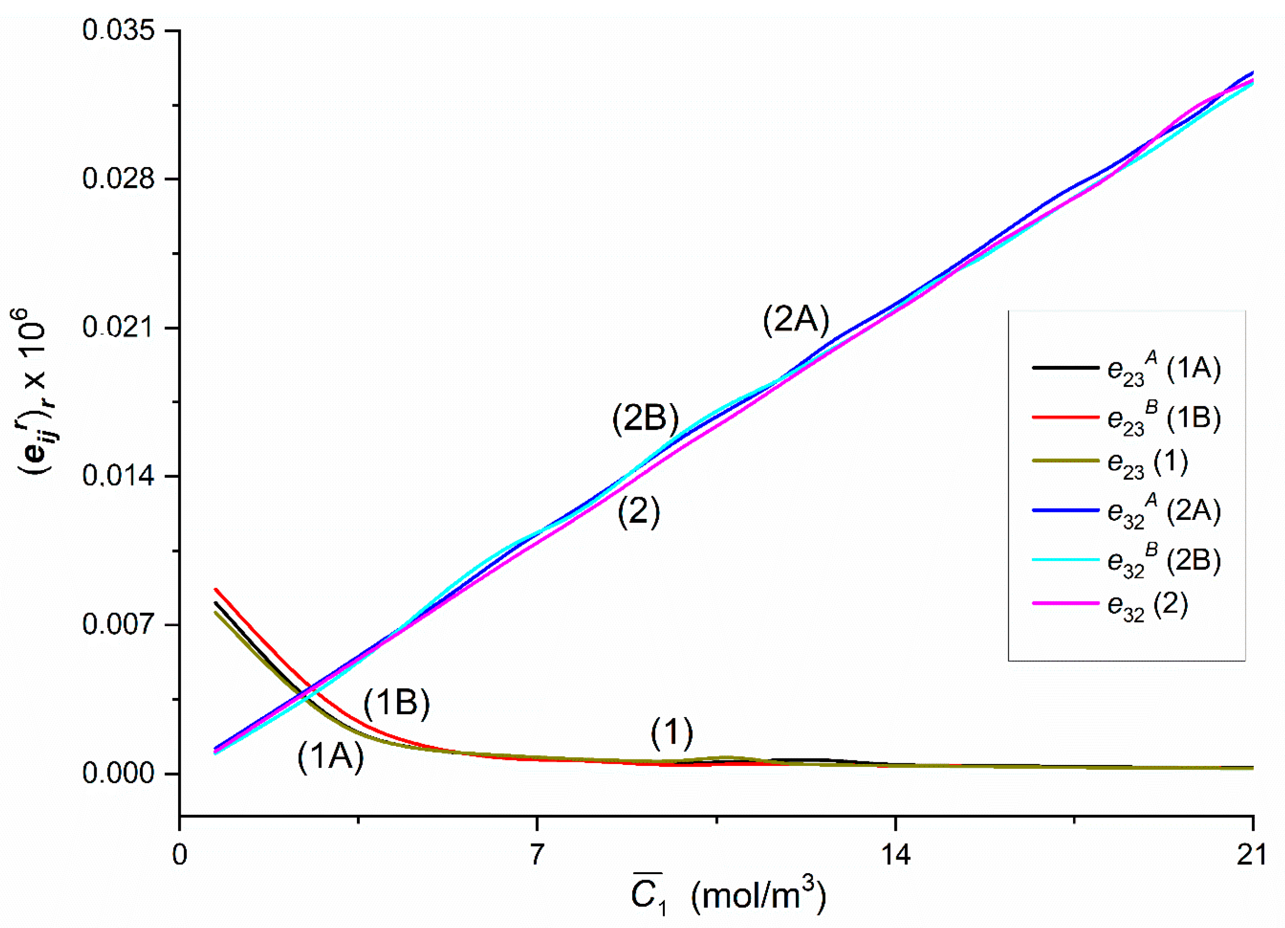
From the course of Curves 1A, 1B and 1 presented in
Figure 19 it follows that
=
=
and
=
=
. Curves 1, 1A and 1B and 2, 2A and 2B intersect at a point with coordinates
=
=
=
=
=
≈ 0.004 and
= 2.57 mol/m
3. For
< 2.57 mol/m
3,
=
=
>
=
=
and for
> 2.57 mol/m
3,
=
=
<
=
=
.
Figure 17,
Figure 18 and
Figure 19 show that Kedem–Caplan relations take the form: 0.005 ≤
=
≤ 0.05, 0.002 ≤
≤ 0.145, 0.006 ≤
≤ 0.068, 0.003 ≤
≤ 0.104, 0.005 ≤
≤ 0.054, 0.004 ≤
=
≤ 0.02, 0.005 ≤
≤ 0.016, 0.004 ≤
≤ 0.02, 0.005 ≤
≤ 0.015, 0.04 ≤
≤ 0.02, 0.003 × 10
−6 ≤
=
=
≤ 0.009 × 10
−6, 0.001 × 10
−6 ≤
=
=
≤ 0.034 × 10
−6. Hence it follows that,
≠
,
≠
,
≈
,
=
,
=
=
≠
=
=
. The values of all coupling coefficients presented in
Figure 14,
Figure 15 and
Figure 16 fulfill the conditions 0 ≤
≤ 1, 0 ≤
≤ 1, 0 ≤
≤ 1, 0 ≤
≤ 1 determined by Roy Caplan [
20].
Figure 20 and
Figure 21 show the dependences
=
f(
,
= 37.71 mol/m
3) and
=
f(
,
= 37.71 mol/m
3), (
i,
j ∈ {1, 2, 3} and
r = A, B) calculated on the basis of Equations (15) and (16) and data presented in
Figure 14,
Figure 15 and
Figure 16.
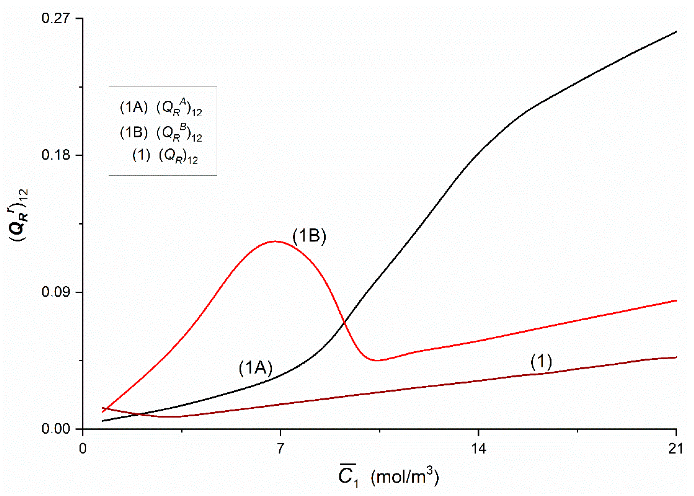
Figure 20 shows that Curves 1A and 1B intersect at a point with coordinates:
=
= 0.07 and
= 9.24 mol/m
3. The course of Curves 1A, 1B and 1 shows that for
< 9.24 mol/m
3,
>
>
and for
> 9.24 mol/m
3,
>
>
. Curve 1B has a maximum. The coordinates of the maximum of Curve 1B are
= 0.12 and
= 6.77 mol/m
3.
Figure 21 shows that Graphs 1A and 1B intersect at the point with the coordinates
=
= 0.015 and
= 9.16 mol/m
3. Curves 1A, 1B and 1 show that for
< 9.24 mol/m
3 >
>
and for
> 9.24 mol/m
3 >
>
. Moreover, it was shown that
=
=
= 0.58 × 10
−8 = constant.
Figure 20 and
Figure 21 show that Kedem–Caplan relations take the form: 0.01 ≤
≤ 0.05, 0.05 ≤
≤ 0.27, 0.01 ≤
≤ 0.13, 0.005 ≤
≤ 0.0055, 0.008 ≤
≤ 0.041, 0.01 ≤
≤ 0.031. The values of all coupling coefficients presented in
Figure 20 and
Figure 21 fulfill the conditions 0 ≤
≤ 1 and 0 ≤
≤ 1.
The results of experimental research indicate that
ω11 >>
ω12,
ω22 >>
ω21,
=
=
= =1,
=
=
=
and
=
=
=
(r = A, B). By accepting the above conditions and that
≈
=
. Given this condition, and Equations (5), (9) and (10), we can write:
Equations (17)–(20) contain the factor
and Equation (22)—the factor
. This factor, using Equation (1) can be written in a form containing the thickness of CBLs. To simplify the accounts, using the conditions
=
=
Dij and
=
=
δr, we write the Equation (1) in the form:
Using Equation (22) we can write:
From all the foregoing considerations, it is clear that coefficients
(
i,
j ∈ {1, 2, 3} and
are measures of the natural convection effect. If the conditions
< 0 and
< 0 are fulfilled, fluxes of natural convection in single-membrane system are directed vertically upwards. In turn, for coefficients
> 0 and
> 0, the fluxes are directed vertically downwards. Zeroing of the coefficients (
= 0 and
= 0) means that the system is in the critical point where the flux turns its direction from vertically upwards to vertically downwards. In this point, the structure of layers lose its stability, but natural convection does not have precise turn yet, what means that the membrane system is not sensitive to changes in the gravitational field. This is shown by dependencies
=
f(
,
= 37.71 mol/m
3), (
i,
j ∈ {1, 2, 3} and
=
f(
,
= 37.71 mol/m
3), presented in
Figure 11,
Figure 12 and
Figure 13 as well as interferograms presented in the previous publication [
37,
38]. Hydrodynamic stability in the membrane system is controlled by the concentration Rayleigh number [
34,
35,
36,
37,
38]. The Rayleigh number value depends on the concentration of solutions separated by the membrane [
34,
35]. For the points where
= 0 and
= 0, (
i,
j ∈ {1, 2, 3}) the critical value of concentration Rayleigh number (
RC) can be specified.
For example, we will consider Equations (20) and (23) and
Figure 2 and
Figure 3 for the
coefficient. This equation can be written as
. It is drawn from the equation and
Figure 2 that if
= 0, then
=
= 0.234. From the equation, it becomes apparent that if
= 0, then
=
. The values of
and
can be determined by laser interferometry [
35,
36,
37,
38] or volume flux measurements [
34].
Figure 3 presents the dependences
=
f(
ρh −
ρl) obtained by converting the dependence
=
f(
= const.) shown in
Figure 3, with the help of equations
and
ρh −
ρl = (∂
ρ/∂
C1)(
C1h −
C1l) + (∂
ρ/∂
C2)(
C2h −
C2l). From this figure it follows that
=
≈ 1.3 × 10
−3 m for
ρh −
ρl = 0.046 kg/m
3.
Let us consider the dependency
=
f(
,
= 37.71 mol/m
3) shown in the
Figure 12. It results from the figure that
= 0 for
= 9.24 mol/m
3 and
= 37.71 mol/m
3. It should be pointed out that
= 9.24 mol/m
3 if
C1h = 33.44 mol/m
3 and
C1l = 1 mol m
−3 while
= 37.71 mol/m
3, for
C2h = 201 mol/m
3 and
C2l = 1 mol/m
3. Therefore, consisting solution density amounts to 998.3 kg/m
3. In turn, kinematic viscosity of this solution is equal to
ν = 1.063 × 10
−6 m
2/s. Density difference of solutions located in the Compartments (h) and (l) calculated on the basis of equation
ρh −
ρl = (∂
ρ/∂
C1)(
C1h −
C1l) + (∂
ρ/∂
C2)(
C2h −
C2l), where (∂
ρ/∂
C1) = 0.06 kg/mol, (∂
ρ/∂
C2) = −0.0095 kg/mol, amounts to
ρh −
ρl = 0.046 kg/m
3. Taking these data into consideration, as well as
D11 = 0.69 × 10
−9 m
2/s,
g = 9.81 m/s
2,
ω11 = 0.8 × 10
−9 mol/Ns,
= 1.3 × 10
−3 m in the expression for the concentration Rayleigh number
RC = [
g(
ρh −
ρl)(
δ)
3](
ρhνhD11)
−1 [
29,
30], we get
RC = 1353.1. This value corresponds to the (
RC)
crit. = 1100.6, obtained for the case of the rigid membrane surface and the free liquid interior (rigid-free borders) [
44,
45]. For electrolysis occurring in a cell containing electrodes placed in parallel in horizontal planes, the critical Rayleigh number depends strongly on the distance between these electrodes and for amperostatic conditions takes the values in the range of
RC = 1070 ÷ 1540 [
46]. In turn, for potentiostatic conditions
RC takes the values in the range of
RC = 763.3 ÷ 1351 [
47].


