Variable Selection and Regularization in Quantile Regression via Minimum Covariance Determinant Based Weights


Abstract
:1. Introduction
- Rather than carrying an "omnibus" study of penalized WQR as in [20,21], we carry out a detailed study by distinguishing different types of high leverage points viz.,
- –
- Collinearity influential points which comprise collinearity inducing and collinearity hiding points.
- –
- High leverage points which are not collinearity influential.
- Taking advantage of high computing power, we make use of the very robust weights based on the computationally intensive high breakdown minimum covariance determinant (MCD) method rather than the well-known classical Mahalanobis distance or any LS based weights as in [20] which are amenable to outliers.
2. Preliminaries
2.1. Quantile Regression
2.2. Variable Selection in Quantile Regression
3. Variable Selection and Regularization in Weighted Quantile Regression
3.1. Choice of Weights for Downweighing High Leverage Observations Motivation
3.2. Penalized Weighted Quantile Regression
3.3. Asymptotic Properties
- (i)
- The regression errors ’s are , with quantile zero and continuous, positive density in a neighborhood of zero (see [31]).
- (ii)
- Let , where for are known positive values that satisfy .
- (iii)
- There exists a positive definite matrix : , where and denote the and top-left and right-bottom submatrices of , respectively.
- (K1)
- As .
- (K2)
- The random error terms ’s are independent with the distribution function of . We assume is locally linear near zero (with a positive slope) and .
- (K3)
- Assume that, for each , , where is a strictly convex function taking values in with denoting a convex function for each n and i.
4. Simulation Study
- − This predictor matrix is obtained from orthogonalization such that . Using singular value decomposition (SVD), we solve , where for and ; U and V are orthogonal with the diagonal entries of D giving the singular (eigen) values of W. Then, is such that due to orthogonality of U.
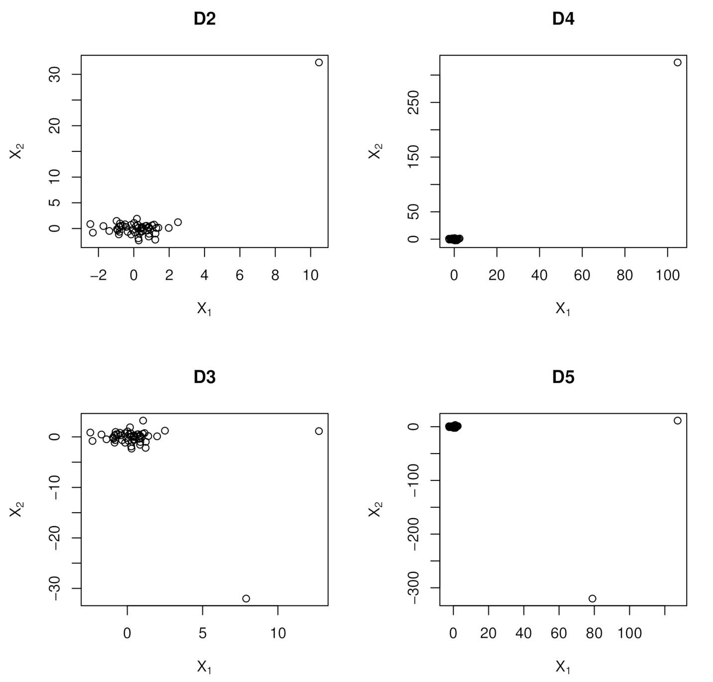
- −has a collinearity inducing point which is , but with observation having the largest Euclidean distance from the center of the design space moved 10 units in the X-space.
- −has collinearity hiding point which is , but with observations having the largest (second largest) Euclidean distance from the center of the design space moved 10 units in the X-space.
- −has a collinearity inducing point which is , but with observation having the largest Euclidean distance from the center of the design space moved 100 units in the X-space.
- −has collinearity hiding point which is , but with observations having the largest (second largest) Euclidean distance from the center of the design space moved 100 units in the X-space.
- −has () correlated and leverage contaminated sub matrices of , i.e., , where with and ( controls the degree of correlation), , is the entry of the covariance matrix , is the correlated sub matrix of ; with is the leverage contaminated sub matrix of .
- .
- , with choices and .
- with choices .
4.1. Results
5. Examples
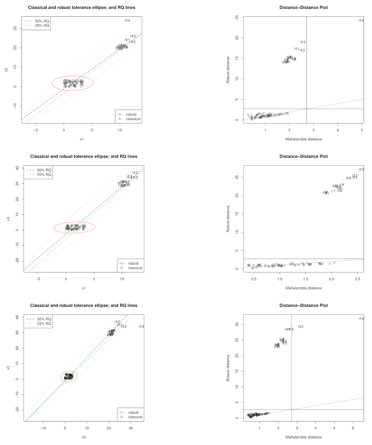
5.1. Hawkins, Bradu, and Kass Data Set
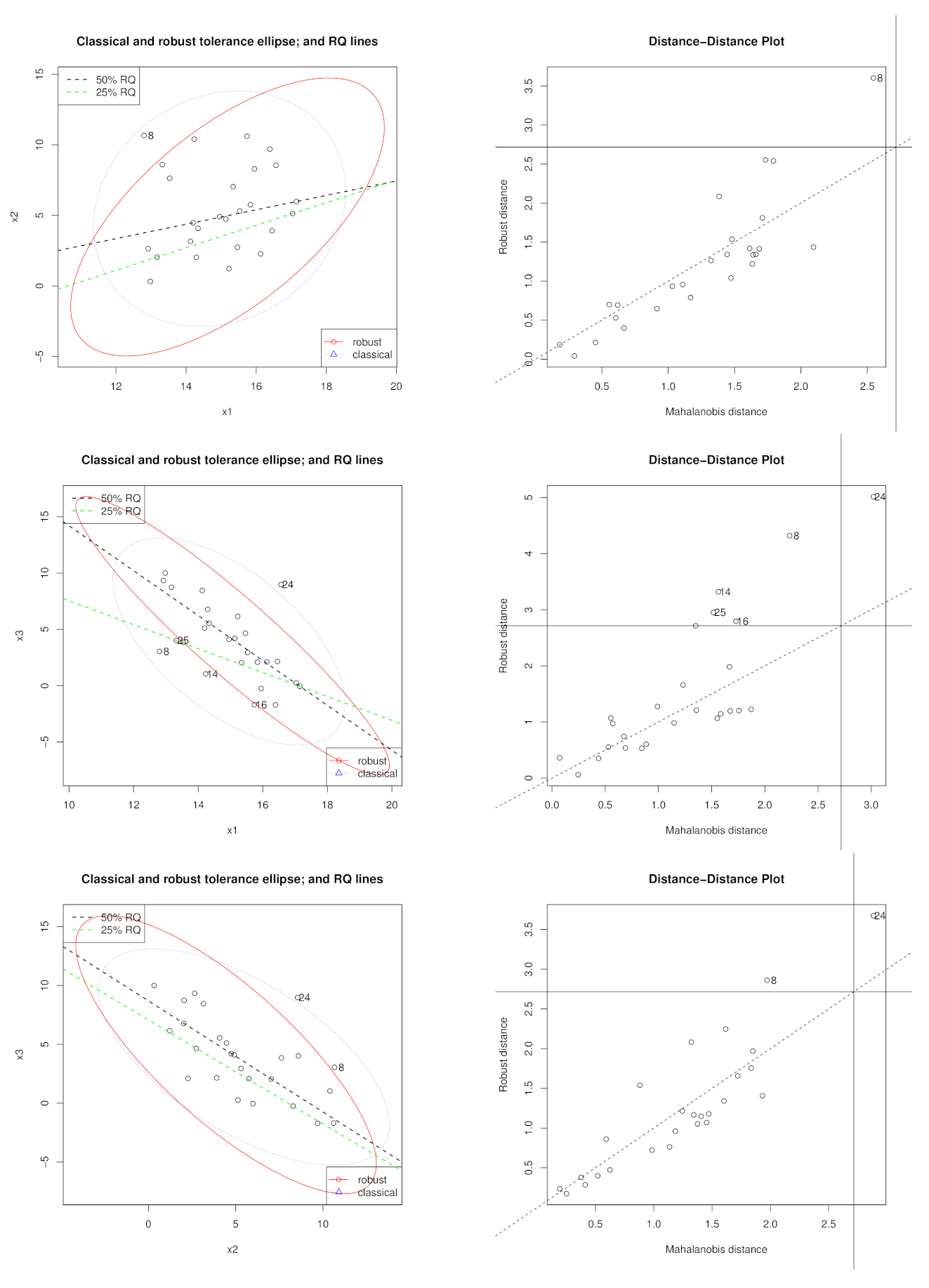
5.2. Hocking and Pendleton Data Set
6. Conclusions
Author Contributions
Funding
Institutional Review Board Statement
Informed Consent Statement
Data Availability Statement
Acknowledgments
Conflicts of Interest
Abbreviations
| LS | Least Squares |
| QR | Quantile Regression |
| RQ | Regression Quantile |
| Regression Quantile at quantile level | |
| WQR | Weighted Quantile Regression |
| LAD | Least Absolute Deviation |
| LP | Linear Programming |
| LASSO | Least Absolute Shrinkage and Selection Operator |
| E-NET | Elastic Net |
| SCAD | Smoothly Clipped Absolute Deviation |
| CQR | Composite Quantile Regression |
| MCD | Minimum Covariance Determinant |
| SVD | Singular value Decomposition |
References
- Koenker, R.W.; Bassett, G. Regression Quantiles. Econometrica 1978, 46, 33–50. [Google Scholar] [CrossRef]
- Yu, K.; Lu, Z.; Stander, J. Quantile regression: Applications and current research areas. J. R. Stat. Soc. Ser. D 2003, 52, 331–350. [Google Scholar] [CrossRef]
- Koenker, R. Econometric Society Monographs: Quantile Regression; Cambridge University: New York, NY, USA, 2005. [Google Scholar]
- Chatterjee, S.; Hadi, A.S. Impact of simultaneous omission of a variable and an observation on a linear regression equation. Comput. Stat. Data Anal. 1988, 6, 129–144. [Google Scholar] [CrossRef]
- Hubert, M.; Rousseeuw, P.J. Robust regression with both continuous and binary regressors. J. Stat. Plan. Inference 1997, 57, 153–163. [Google Scholar] [CrossRef]
- Salibián-Barrera, M.; Wei, Y. Weighted quantile regression with nonelliptically structured covariates. Can. J. Stat. 2008, 36, 595–611. [Google Scholar] [CrossRef]
- Hoerl, A.E.; Kennard, R.W. Ridge Regression: Biased Estimation for Nonorthogonal Problems. Technometrics 1970, 12, 55–67. [Google Scholar] [CrossRef]
- Wang, H.; Li, G.; Jiang, G. Robust Regression Shrinkage and Consistent Variable Selection through the LAD-Lasso. J. Bus. Econ. Stat. 2007, 25, 347–355. [Google Scholar] [CrossRef]
- Tibshirani, R. Regression Shrinkage and Selection via the Lasso. J. R. Stat. Soc. Ser. B 1996, 58, 267–288. [Google Scholar] [CrossRef]
- Obuchi, T.; Kabashima, Y. Cross validation in {LASSO} and its acceleration. J. Stat. Mech. Theory Exp. 2016, 2016, 53304. [Google Scholar] [CrossRef]
- Zou, H.; Hastie, T. Regularization and variable selection via the Elastic Net. J. R. Stat. Soc. Ser. B 2005, 67, 301–320. [Google Scholar] [CrossRef] [Green Version]
- Yi, C.; Huang, J. Semismooth Newton Coordinate Descent Algorithm for Elastic-Net Penalized Huber Loss Regression and Quantile Regression. J. Comput. Graph. Stat. 2017, 26, 547–557. [Google Scholar] [CrossRef] [Green Version]
- Wu, Y.; Liu, Y. Variable selection in quantile regression. Stat. Sin. 2009, 19, 801–817. [Google Scholar]
- Jiang, X.; Jiang, J.; Song, X. Oracle model selection for nonlinear models based on weighted composite quantile regression. Stat. Sinica 2012, 22, 1479–1506. [Google Scholar]
- Zou, H. The Adaptive Lasso and Its Oracle Properties. J. Am. Stat. Assoc. 2006, 101, 1418–1429. [Google Scholar] [CrossRef] [Green Version]
- Tibshirani, R.; Saunders, M.; Rosset, S.; Zhu, J.; Knight, K. Sparsity and smoothness via the fused lasso. J. R. Stat. Soc. Ser. B 2005, 67, 91–108. [Google Scholar] [CrossRef] [Green Version]
- Yuan, M.; Lin, Y. Model selection and estimation in regression with grouped variables. J. R. Stat. Soc. Ser. B 2006, 68, 49–67. [Google Scholar] [CrossRef]
- Belloni, A.; Chernozhukov, V. ℓ1-penalized quantile regression in high-himensional sparse models. Ann. Stat. 2011, 39, 82–130. [Google Scholar] [CrossRef]
- Zou, H.; Yuan, M. Composite quantile regression and the oracle model selection theory. Ann. Stat. 2008, 36, 1108–1126. [Google Scholar] [CrossRef]
- Arslan, O. Weighted LAD-LASSO method for robust parameter estimation and variable selection in regression. Comput. Stat. Data Anal. 2012, 56, 1952–1965. [Google Scholar] [CrossRef]
- Norouzirad, M.; Hossain, S.; Arashi, M. Shrinkage and penalized estimators in weighted least absolute deviations regression models. J. Stat. Comput. Simul. 2018, 88, 1557–1575. [Google Scholar] [CrossRef]
- Hoerl, A.E.; Kannard, R.W.; Baldwin, K.F. Ridge regression:some simulations. Commun. Stat. 1975, 4, 105–123. [Google Scholar] [CrossRef]
- Lawless, J.F.; Wang, P. A simulation study of ridge and other regression estimators. Commun. Stat. Theory Methods 1976, 5, 307–323. [Google Scholar] [CrossRef]
- Hocking, R.R.; Speed, F.M.; Lynn, M.J. A Class of Biased Estimators in Linear Regression. Technometrics 1976, 18, 425–437. [Google Scholar] [CrossRef]
- Kibria, B.M.G. Performance of Some New Ridge Regression Estimators. Commun. Stat. Simul. Comput. 2003, 32, 419–435. [Google Scholar] [CrossRef]
- Khalaf, G.; Shukur, G. Choosing Ridge Parameter for Regression Problems. Commun. Stat. Theory Methods 2005, 34, 1177–1182. [Google Scholar] [CrossRef]
- Rousseeuw, P.J.; Leroy, A.M. Robust Regression and Outlier Detection; John Wiley & Sons: Hoboken, NY, USA, 2005; Volume 589. [Google Scholar]
- Rousseeuw, P. Multivariate Estimation with High Breakdown Point. Math. Stat. Appl. 1985, 283–297. [Google Scholar] [CrossRef]
- Rousseeuw, P.J.; Hubert, M. Anomaly detection by robust statistics. WIREs Data Min. Knowl. Discov. 2018, 8, e1236. [Google Scholar] [CrossRef] [Green Version]
- Giloni, A.; Simonoff, J.S.; Sengupta, B. Robust weighted LAD regression. Comput. Stat. Data Anal. 2006, 50, 3124–3140. [Google Scholar] [CrossRef] [Green Version]
- Pollard, D. Asymptotics for Least Absolute Deviation Regression Estimators. Econom. Theory 1991, 7, 186–199. [Google Scholar] [CrossRef]
- Knight, K. Asymptotics for L1-estimators of regression parameters under heteroscedasticityY. Can. J. Stat. 1999, 27, 497–507. [Google Scholar] [CrossRef]
- Ranganai, E.; Van Vuuren, J.O.; De Wet, T. Multiple case high leverage diagnosis in regression quantiles. Commun. Stat. Theory Methods 2014, 43, 3343–3370. [Google Scholar] [CrossRef] [Green Version]
- Yi, C. Hqreg: Regularization Paths for Huber Loss Regression and Quantile Regression Penalized by Lasso or Elastic-Net; R Package Version 1.3; R-CRAN Repository; 2016; Available online: https://cran.r-project.org/web/packages/hqreg/index.html (accessed on 28 October 2020).
- Hawkins, D.M.; Bradu, D.; Kass, G.V. Location of Several Outliers in Multiple-Regression Data Using Elemental Sets. Technometrics 1984, 26, 197–208. [Google Scholar] [CrossRef]
- Hocking, R.; Pendleton, O. The regression dilemma. Commun. Stat. Theory Methods 1983, 12, 497–527. [Google Scholar] [CrossRef]
- Bagheri, A.; Habshah, M.; Imon, R. A novel collinearity-influential observation diagnostic measure based on a group deletion approach. Commun. Stat. Simul. Comput. 2012, 41, 1379–1396. [Google Scholar] [CrossRef]


| Correctly | No. of Zeros | Med (MAD) | |||||
|---|---|---|---|---|---|---|---|
| Parameters | Method | Fitted | Correct | Incorrect | Test Error | Optimal | |
| D1 under the Normal Distribution | , | QR-RIDGE | 0 | 2.27 | 0 | 1.28(1.97) | 0.12 |
| QR-LASSO | 67.5 | 4.56 | 0 | 0.71(1.20) | 0.04 | ||
| QR-E-NET | 18.5 | 3.59 | 0 | 0.72(1.25) | 0.04 | ||
| , | QR-RIDGE | 1.5 | 2.33 | 0 | −0.03(1.99) | 0.14 | |
| QR-LASSO | 62 | 4.49 | 0 | 0.00(1.15) | 0.05 | ||
| QR-E-NET | 24 | 3.6 | 0 | 0.01(1.19) | 0.04 | ||
| , | QR-RIDGE | 9 | 3.07 | 0.03 | 2.70(4.32) | 0.12 | |
| QR-LASSO | 39.5 | 4.52 | 0.38 | 2.03(3.60) | 0.04 | ||
| QR-E-NET | 30.5 | 4 | 0.2 | 2.18(3.69) | 0.04 | ||
| , | QR-RIDGE | 2.5 | 2.37 | 0.01 | −0.04(4.06) | 0.12 | |
| QR-LASSO | 40 | 4.57 | 0.32 | 0.01(3.45) | 0.05 | ||
| QR-E-NET | 31 | 3.9 | 0.11 | 0.00(3.55) | 0.04 | ||
| D1 under the t Distribution | , , | QR-RIDGE | 3.00 | 2.33 | 0.02 | 2.17(3.21) | 0.11 |
| QR-LASSO | 64.00 | 4.92 | 0.72 | 1.24(2.16) | 0.04 | ||
| QR-E-NET | 36.50 | 4.42 | 0.62 | 1.44(2.41) | 0.03 | ||
| , , | QR-RIDGE | 1.50 | 2.56 | 0.01 | 0.02(2.94) | 0.13 | |
| QR-LASSO | 64.50 | 4.94 | 0.67 | 0.02(1.72) | 0.04 | ||
| QR-E-NET | 32.50 | 4.33 | 0.58 | −0.01(1.94) | 0.03 | ||
| , , | QR-RIDGE | 2.50 | 2.37 | 0.03 | 3.05(4.30) | 0.11 | |
| QR-LASSO | 30.50 | 4.95 | 1.57 | 2.44(3.80) | 0.04 | ||
| QR-E-NET | 26.00 | 4.78 | 1.49 | 2.62(4.04) | 0.03 | ||
| , , | QR-RIDGE | 3.50 | 2.49 | 0.02 | 0.02(4.15) | 0.12 | |
| QR-LASSO | 33.50 | 4.95 | 1.38 | 0.02(3.34) | 0.04 | ||
| QR-E-NET | 25.50 | 4.66 | 1.27 | 0.02(3.58) | 0.03 | ||
| UNWEIGHTED | ||||||||||
|---|---|---|---|---|---|---|---|---|---|---|
| NONE-BIASED | RIDGE | LASSO | E-NET | |||||||
| 0.00 | 0.00 | 0.00 | 0.00 | |||||||
| RQ | 0.00 | 2.27 | −2.27 | 2.39 | −2.39 | 2.39 | −2.39 | 2.39 | −2.39 | |
| 2.00 | 1.39 | 0.61 | 1.45 | 0.55 | 1.45 | 0.55 | 1.45 | 0.55 | ||
| 2.00 | 1.87 | 0.13 | 1.79 | 0.21 | 1.79 | 0.21 | 1.79 | 0.21 | ||
| 0.00 | −0.78 | 0.78 | −0.74 | 0.74 | −0.74 | 0.74 | −0.74 | 0.74 | ||
| 0.00 | 0.00 | 0.00 | 0.00 | |||||||
| RQ | −1.00 | 1.09 | −2.09 | 1.32 | −2.32 | 1.32 | −2.32 | 1.32 | −2.32 | |
| 2.00 | 1.59 | 0.41 | 1.48 | 0.52 | 1.48 | 0.52 | 1.48 | 0.52 | ||
| 2.00 | 1.94 | 0.06 | 1.80 | 0.20 | 1.80 | 0.20 | 1.80 | 0.20 | ||
| 0.00 | −0.88 | 0.88 | −0.76 | 0.76 | −0.76 | 0.76 | −0.76 | 0.76 | ||
| WEIGHTED | ||||||||||
| NONE-BIASED | RIDGE | LASSO | E-NET | |||||||
| 0.00 | 0.00 | 0.06 | 0.00 | |||||||
| RQ | 0.00 | 2.27 | −2.27 | 0.11 | −0.11 | 0.00 | 0.00 | 0.11 | −0.11 | |
| 2.00 | 1.39 | 0.61 | 1.93 | 0.07 | 1.93 | 0.07 | 1.93 | 0.07 | ||
| 2.00 | 1.87 | 0.13 | 2.01 | −0.01 | 1.97 | 0.03 | 2.01 | −0.01 | ||
| 0.00 | −0.78 | 0.78 | −0.09 | 0.09 | 0.00 | 0.00 | −0.09 | 0.09 | ||
| 0.00 | 0.50 | 0.50 | 0.50 | |||||||
| RQ | −1.00 | 1.09 | −2.09 | 0.18 | −1.18 | 0.29 | −1.29 | 0.29 | −1.29 | |
| 2.00 | 1.59 | 0.41 | 0.35 | 1.65 | 0.00 | 2.00 | 0.00 | 2.00 | ||
| 2.00 | 1.94 | 0.06 | 0.39 | 1.61 | 0.00 | 2.00 | 0.00 | 2.00 | ||
| 0.00 | −0.88 | 0.88 | 0.38 | −0.38 | 0.00 | 0.00 | 0.00 | 0.00 | ||
| UNWEIGHTED | ||||||||||
|---|---|---|---|---|---|---|---|---|---|---|
| NONE-BIASED | RIDGE | LASSO | E-NET | |||||||
| 0.00 | 0.00 | 0.00 | 0.00 | |||||||
| RQ | intercept | 0.00 | 0.74 | −0.74 | 0.50 | −0.50 | 0.50 | −0.50 | 0.50 | −0.50 |
| 2.00 | 1.86 | 0.14 | 1.84 | 0.16 | 1.84 | 0.16 | 1.84 | 0.16 | ||
| 2.00 | 1.93 | 0.07 | 1.87 | 0.13 | 1.87 | 0.13 | 1.87 | 0.13 | ||
| 0.00 | −0.07 | 0.07 | −0.03 | 0.03 | −0.03 | 0.03 | −0.03 | 0.03 | ||
| 0.00 | 0.00 | 0.00 | 0.00 | |||||||
| RQ | intercept | −1.00 | 0.69 | −1.69 | −0.09 | −0.91 | −0.09 | 0.09 | −0.09 | −0.91 |
| 2.00 | 1.67 | 0.33 | 1.73 | 0.27 | 1.73 | 0.27 | 1.73 | 0.27 | ||
| 2.00 | 1.90 | 0.10 | 1.95 | 0.05 | 1.95 | 0.05 | 1.95 | 0.05 | ||
| 0.00 | −0.08 | 0.08 | −0.10 | 0.10 | −0.10 | 0.10 | −0.10 | 0.10 | ||
| WEIGHTED | ||||||||||
| NONE-BIASED | RIDGE | LASSO | E-NET | |||||||
| 0.00 | 0.00 | 0.00 | 0.00 | |||||||
| RQ | intercept | 0.00 | 0.74 | −0.74 | 0.27 | −0.27 | 0.27 | −0.27 | 0.27 | −0.27 |
| 2.00 | 1.86 | 0.14 | 1.86 | 0.14 | 1.86 | 0.14 | 1.86 | 0.14 | ||
| 2.00 | 1.93 | 0.07 | 1.96 | 0.04 | 1.96 | 0.04 | 1.96 | 0.04 | ||
| 0.00 | −0.07 | 0.07 | −0.06 | 0.06 | −0.06 | 0.06 | −0.06 | 0.06 | ||
| 0.00 | 0.50 | 0.33 | 0.50 | |||||||
| RQ | intercept | −1.00 | 0.69 | −1.69 | 1.74 | −2.74 | 2.22 | −3.22 | 2.20 | −3.20 |
| 2.00 | 1.67 | 0.33 | 0.30 | 1.70 | 0.00 | 2.00 | 0.00 | 2.00 | ||
| 2.00 | 1.90 | 0.10 | 0.48 | 1.52 | 0.00 | 2.00 | 0.10 | 1.90 | ||
| 0.00 | −0.08 | 0.08 | 0.22 | −0.22 | 0.00 | 0.00 | 0.00 | 0.00 | ||
| UNWEIGHTED | ||||||||||
|---|---|---|---|---|---|---|---|---|---|---|
| NONE-BIASED | RIDGE | LASSO | E-NET | |||||||
| 0.00 | 0.11 | 0.06 | 0.11 | |||||||
| RQ | intercept | 0.00 | 25.09 | −25.09 | 24.34 | −24.34 | 27.63 | −27.63 | 23.63 | −23.63 |
| 3.00 | 1.55 | 1.45 | 0.86 | 2.14 | 1.28 | 1.72 | 1.06 | 1.94 | ||
| −2.00 | −2.30 | 0.30 | −0.86 | −1.14 | −2.12 | 0.12 | −1.21 | −0.79 | ||
| 0.00 | −0.66 | 0.66 | 0.17 | −0.17 | −0.49 | 0.49 | 0.00 | 0.00 | ||
| 0.00 | 0.00 | 0.06 | 0.06 | |||||||
| RQ | intercept | −1.00 | 23.53 | −24.53 | 25.26 | −26.26 | 30.32 | −31.32 | 33.13 | −34.13 |
| 3.00 | 1.19 | 1.81 | 1.09 | 1.91 | 0.56 | 2.44 | 0.30 | 2.70 | ||
| −2.00 | −1.96 | −0.04 | −1.98 | −0.02 | −1.70 | −0.30 | −1.53 | −0.47 | ||
| 0.00 | −0.15 | 0.15 | −0.16 | 0.16 | 0.00 | 0.00 | 0.02 | −0.02 | ||
| WEIGHTED | ||||||||||
| NONE-BIASED | WQR-RIDGE | WQR-LASSO | WQR-E-NET | |||||||
| RQ | intercept | 0.00 | 25.09 | −25.09 | 0.36 | −0.36 | 0.36 | −0.36 | 0.36 | −0.36 |
| 3.00 | 1.55 | 1.45 | 2.94 | 0.06 | 2.94 | 0.06 | 2.94 | 0.06 | ||
| −2.00 | −2.30 | 0.30 | −2.08 | 0.08 | −2.08 | 0.08 | −2.08 | 0.08 | ||
| 0.00 | −0.66 | 0.66 | 0.01 | −0.01 | 0.01 | −0.01 | 0.01 | −0.01 | ||
| 0.00 | 0.00 | 0.00 | 0.00 | |||||||
| RQ | intercept | −1.00 | 23.53 | −24.53 | −0.08 | −0.92 | −0.08 | −0.92 | 7.62 | −8.62 |
| 3.00 | 1.19 | 1.81 | 2.95 | 0.05 | 2.95 | 0.05 | 2.95 | 0.05 | ||
| −2.00 | −1.96 | −0.04 | −2.47 | 0.47 | −2.47 | 0.47 | −2.47 | 0.47 | ||
| 0.00 | −0.15 | 0.15 | −0.03 | 0.03 | −0.03 | 0.03 | −0.03 | 0.03 | ||
| UNWEIGHTED | ||||||||||
|---|---|---|---|---|---|---|---|---|---|---|
| NONE-BIASED | RIDGE | LASSO | E-NET | |||||||
| 0.00 | 0.00 | 0.22 | 0.08 | |||||||
| RQ | intercept | 0.00 | −59.31 | 59.31 | −56.47 | 56.47 | 40.67 | −40.67 | 8.77 | −8.77 |
| 3.00 | 5.78 | −2.78 | 5.65 | −2.65 | 0.00 | 3.00 | 2.09 | 0.91 | ||
| −2.00 | −0.22 | −1.78 | −0.32 | −1.68 | −1.18 | −0.82 | −1.37 | −0.63 | ||
| 0.00 | 2.13 | −2.13 | 2.05 | −2.05 | 0.00 | 0.00 | 0.30 | −0.30 | ||
| 0.00 | 0.00 | 0.00 | 0.00 | |||||||
| RQ | intercept | −1.00 | −56.16 | 55.16 | −59.60 | 58.60 | −59.61 | 58.61 | −59.61 | 58.61 |
| 3.00 | 5.67 | −2.67 | 5.80 | −2.80 | 5.80 | −2.80 | 5.80 | −2.80 | ||
| −2.00 | −0.61 | −1.39 | −0.48 | −1.52 | −0.48 | −1.52 | −0.48 | −1.52 | ||
| 0.00 | 1.96 | −1.96 | 2.13 | −2.13 | 2.13 | −2.13 | 2.13 | −2.13 | ||
| WEIGHTED | ||||||||||
| NONE-BIASED | WQR-RIDGE | WQR-LASSO | WQR-E-NET | |||||||
| 0.00 | 0.00 | 0.06 | 0.00 | |||||||
| RQ | intercept | 0.00 | −59.31 | 59.31 | 0.12 | −0.12 | −0.24 | 0.24 | 0.12 | −0.12 |
| 3.00 | 5.78 | −2.78 | 2.88 | 0.12 | 2.77 | 0.23 | 2.88 | 0.12 | ||
| −2.00 | −0.22 | −1.78 | −1.88 | −0.12 | −1.44 | −0.56 | −1.88 | −0.12 | ||
| 0.00 | 2.13 | −2.13 | 0.07 | −0.07 | 0.20 | −0.20 | 0.07 | −0.07 | ||
| 0.00 | 0.00 | 0.00 | 0.00 | |||||||
| RQ | intercept | −1.00 | −56.16 | 55.16 | −0.37 | −0.63 | −0.37 | −0.63 | −0.37 | −0.63 |
| 3.00 | 5.67 | −2.67 | 3.02 | −0.02 | 3.02 | −0.02 | 3.02 | −0.02 | ||
| −2.00 | −0.61 | −1.39 | −2.59 | 0.59 | −2.59 | 0.59 | −2.59 | 0.59 | ||
| 0.00 | 1.96 | −1.96 | −0.12 | 0.12 | −0.12 | 0.12 | −0.12 | 0.12 | ||
Publisher’s Note: MDPI stays neutral with regard to jurisdictional claims in published maps and institutional affiliations. |
© 2020 by the authors. Licensee MDPI, Basel, Switzerland. This article is an open access article distributed under the terms and conditions of the Creative Commons Attribution (CC BY) license (http://creativecommons.org/licenses/by/4.0/).
Share and Cite
Ranganai, E.; Mudhombo, I. Variable Selection and Regularization in Quantile Regression via Minimum Covariance Determinant Based Weights. Entropy 2021, 23, 33. https://doi.org/10.3390/e23010033
Ranganai E, Mudhombo I. Variable Selection and Regularization in Quantile Regression via Minimum Covariance Determinant Based Weights. Entropy. 2021; 23(1):33. https://doi.org/10.3390/e23010033
Chicago/Turabian StyleRanganai, Edmore, and Innocent Mudhombo. 2021. "Variable Selection and Regularization in Quantile Regression via Minimum Covariance Determinant Based Weights" Entropy 23, no. 1: 33. https://doi.org/10.3390/e23010033