
Selection of the Optimal Number of Topics for LDA Topic Model—Taking Patent Policy Analysis as an Example


Abstract
:1. Introduction
2. Literature Review
- Doc 1 = [‘apple’, ‘pear’, ‘pear’, ‘apple’, ‘dog’]
- Doc 2 = [‘cat’, ‘dog’, ‘pig’, ‘cat’, ‘dog’]
- Doc 3 = [‘apple’, ‘pear’, ‘apple’, ‘dog’]
- Doc 4 = [‘pig’, ‘dog’, ‘dog’].
- Test1 = [‘pear’, ‘apple’, ‘pig’]
- Test2 = [‘cat’, ‘dog’].
3. LDA Topic Model and Optimal Topic Number Selection Method
3.1. Latent Dirichlet Allocation (LDA)
3.2. Optimal Topic Number Selection Method
3.2.1. Perplexity
3.2.2. Isolation
3.2.3. Stability
Topic Word Ranking Similarity Measurement
Stability of the Topic Model
3.2.4. Coincidence
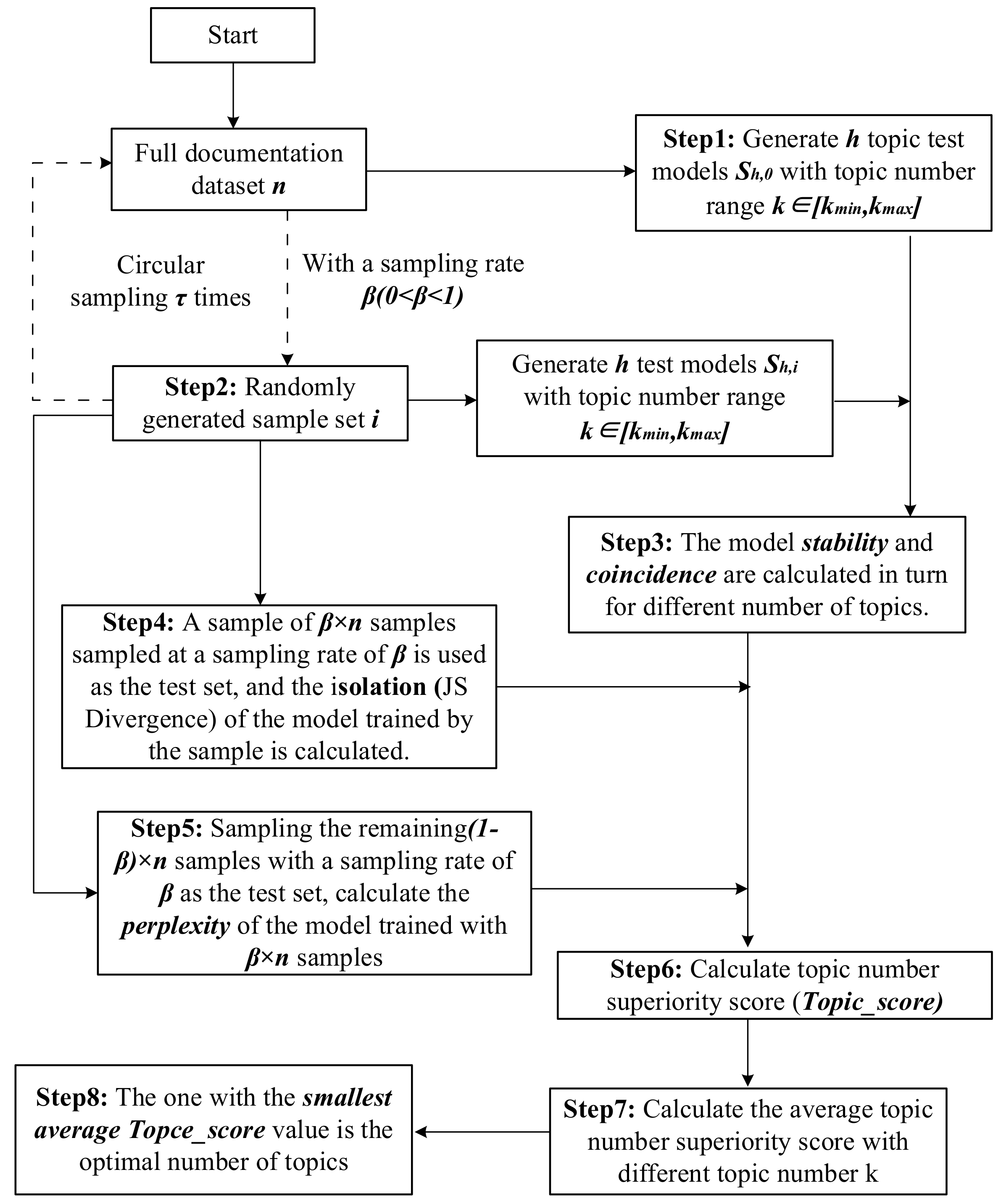
3.2.5. Optimal Topic Number Selection
4. Experimental Analysis and Comparison
4.1. Data Source
4.2. LDA Model Training
4.3. Comparison of Experimental Results
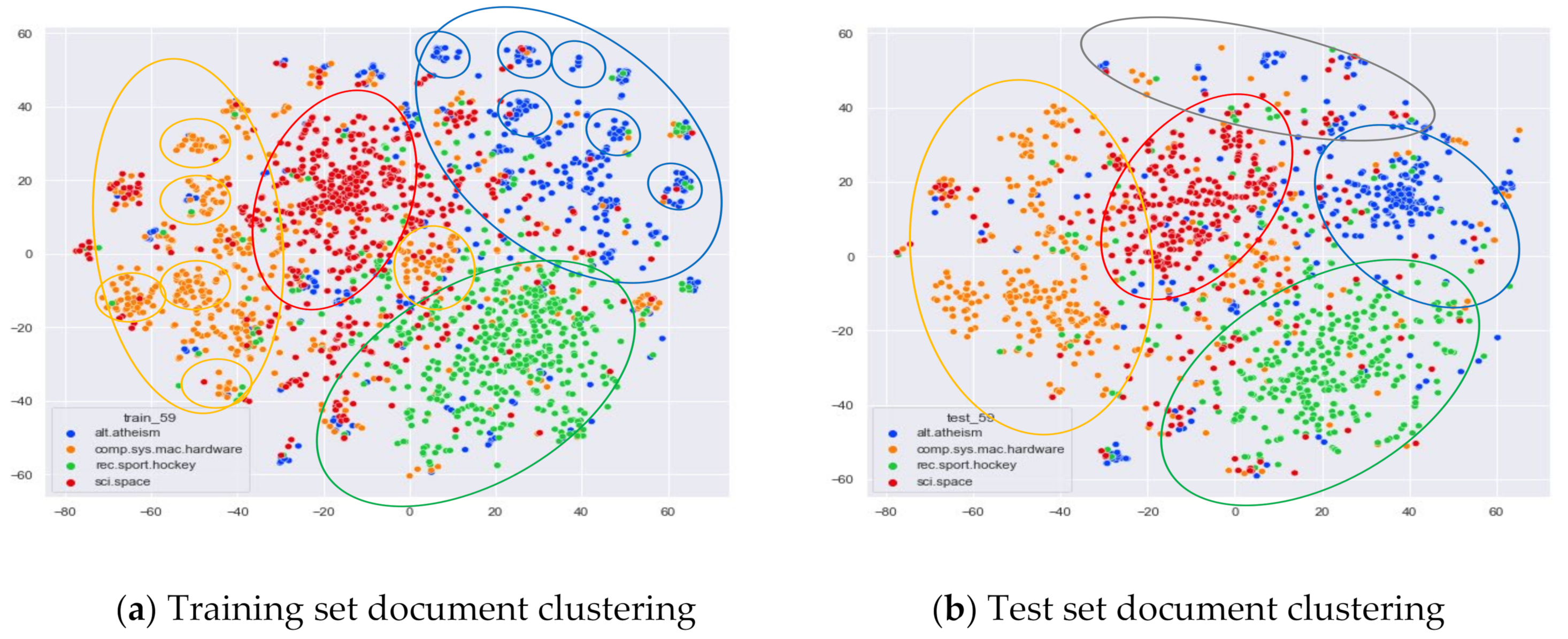
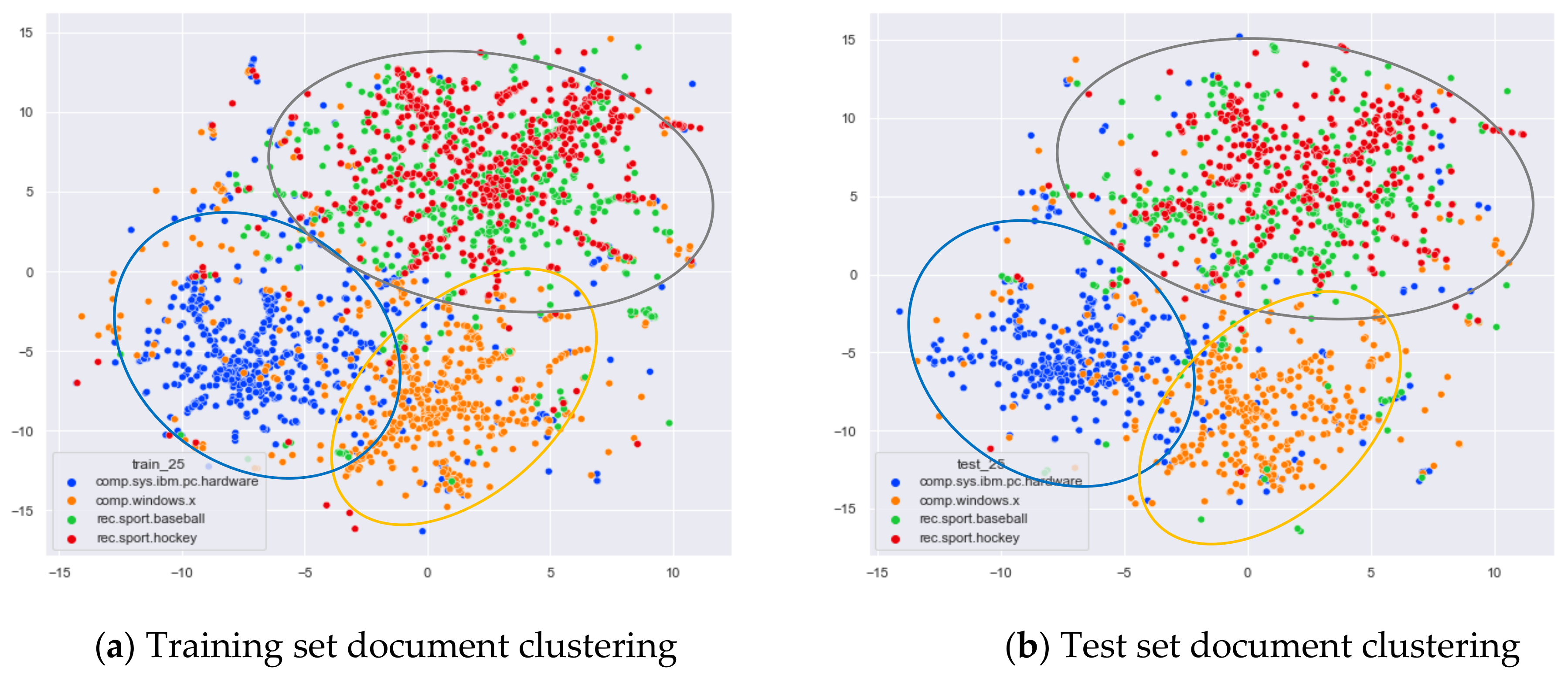
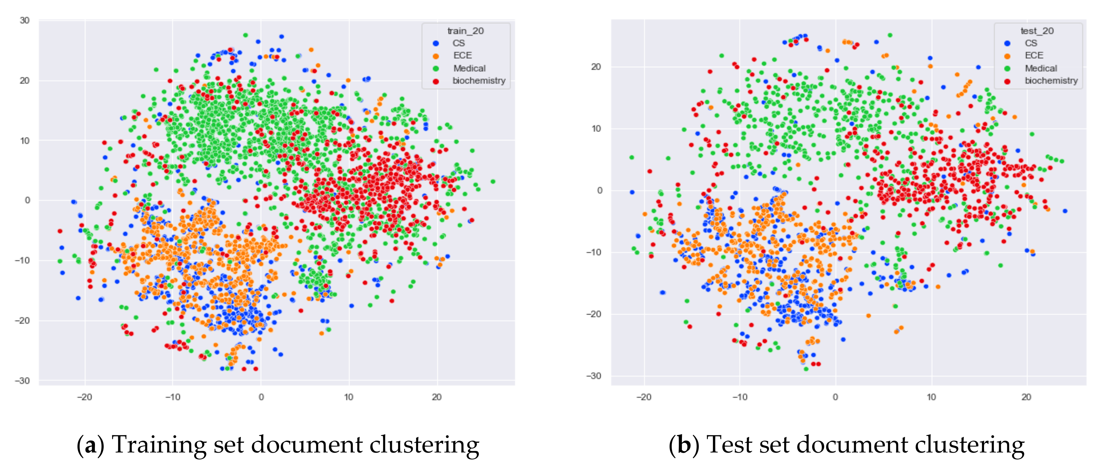
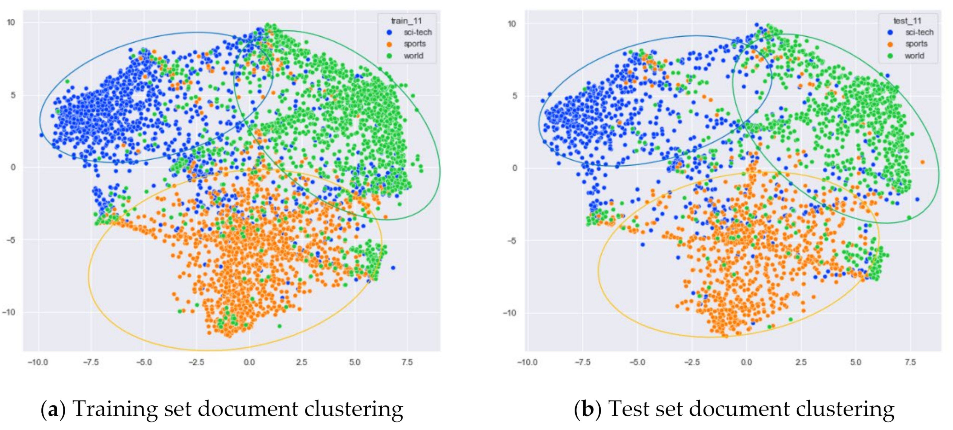
4.3.1. The Experimental Results of 20News_Groups
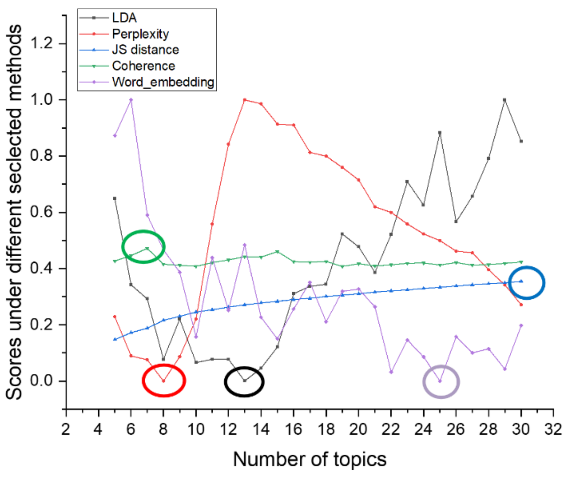
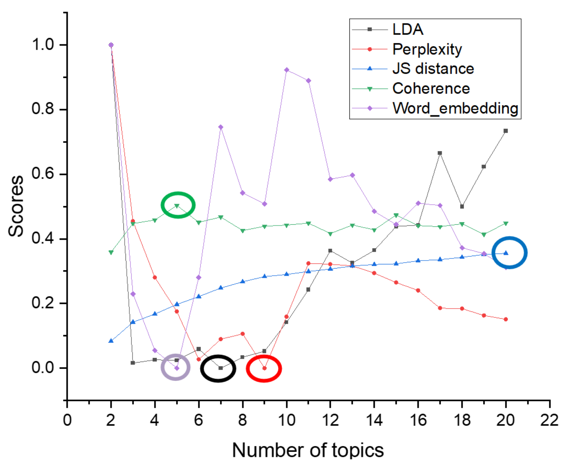
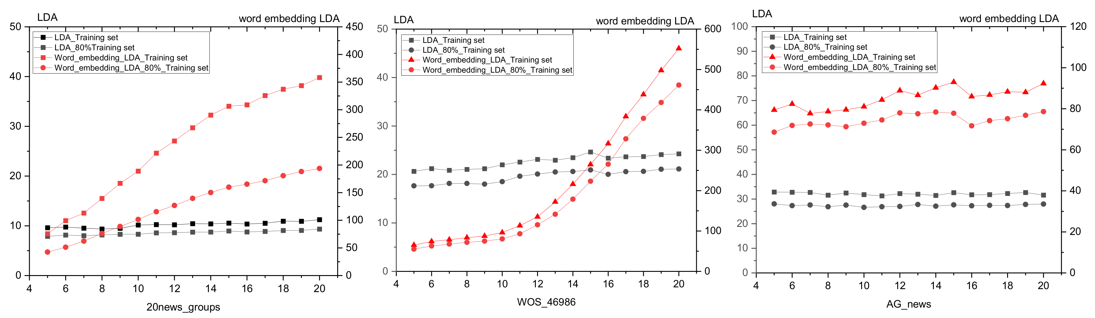
Comparison of Different Topics Number Selection Methods
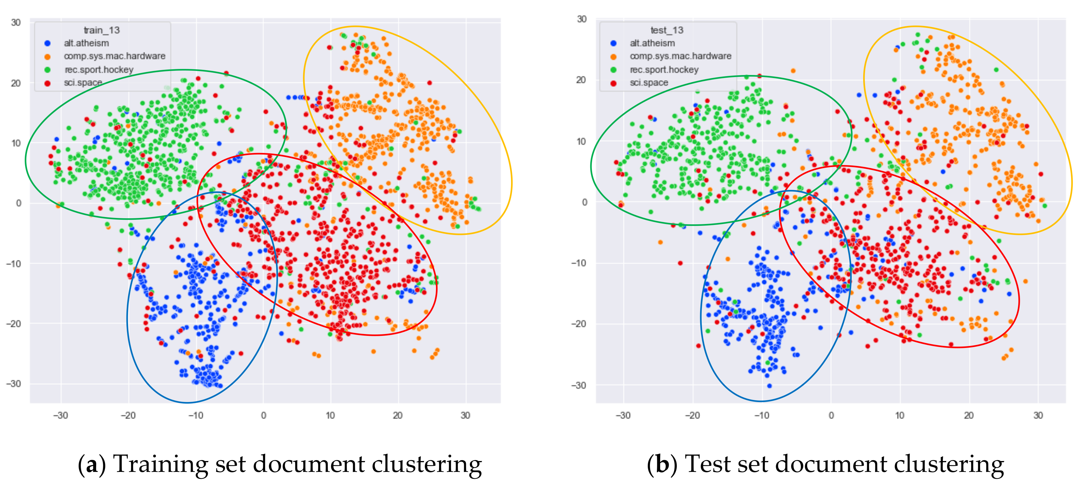
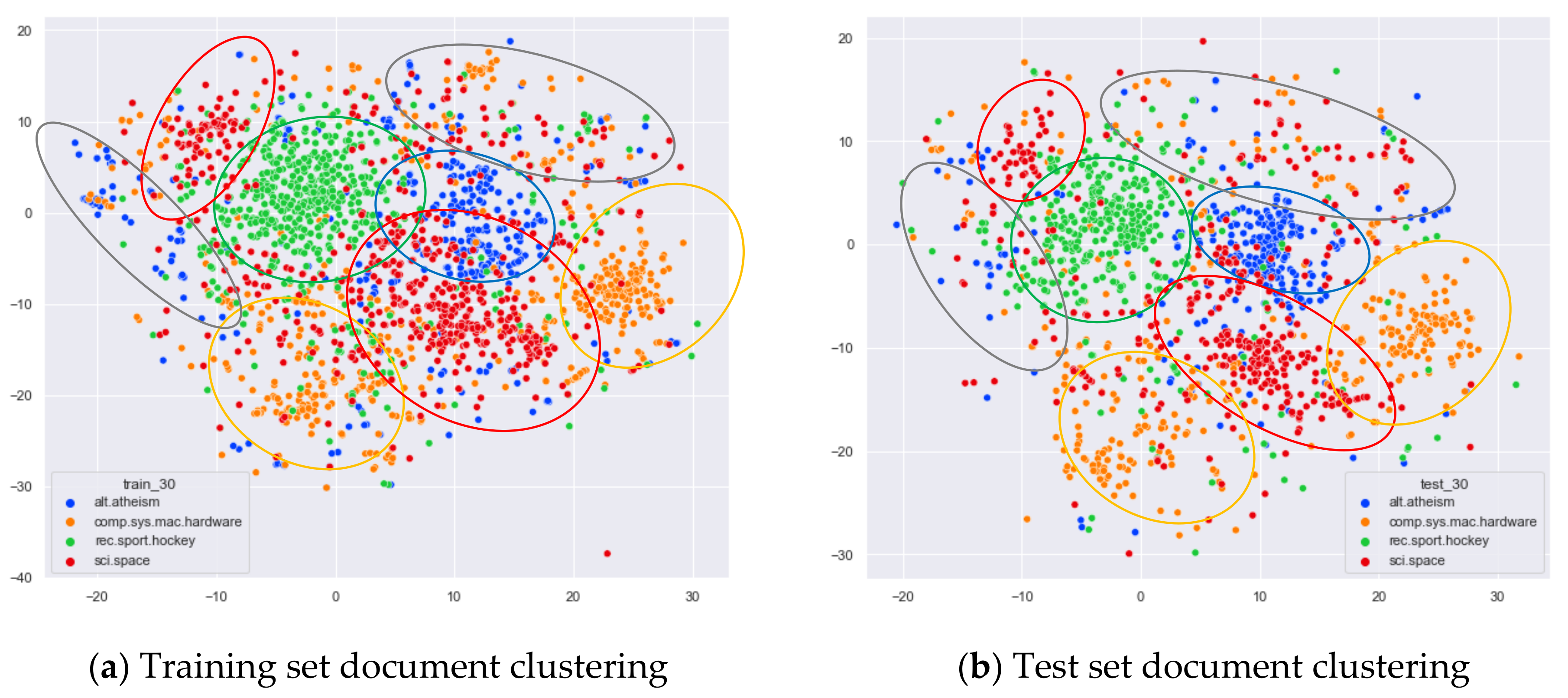
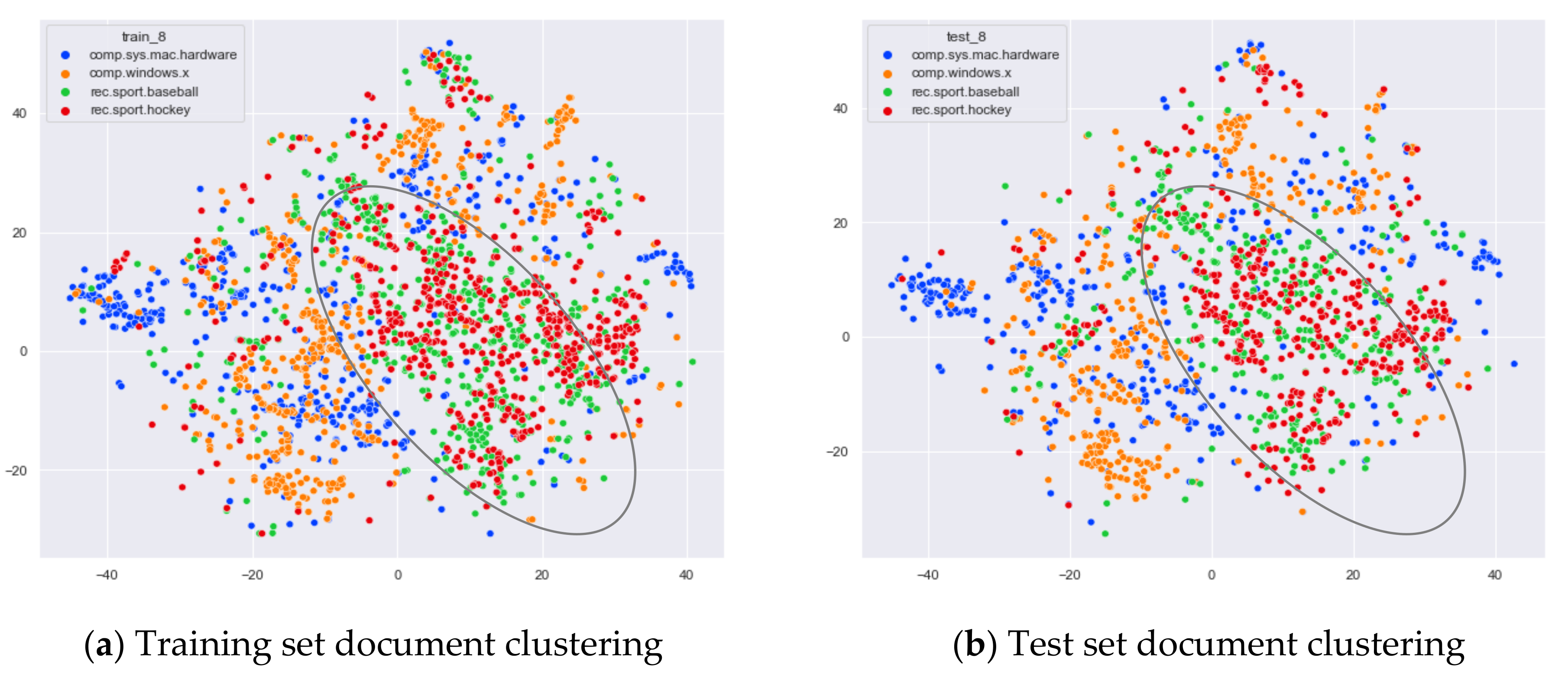
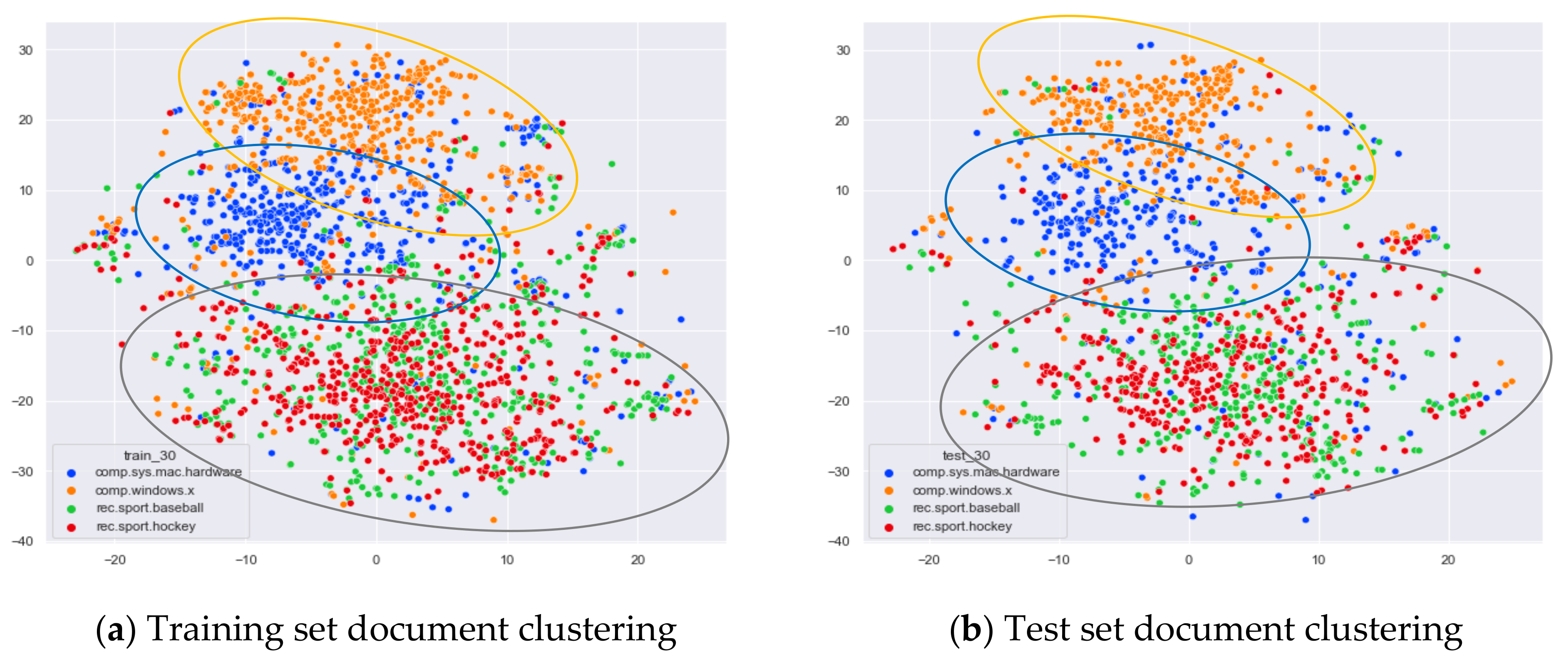
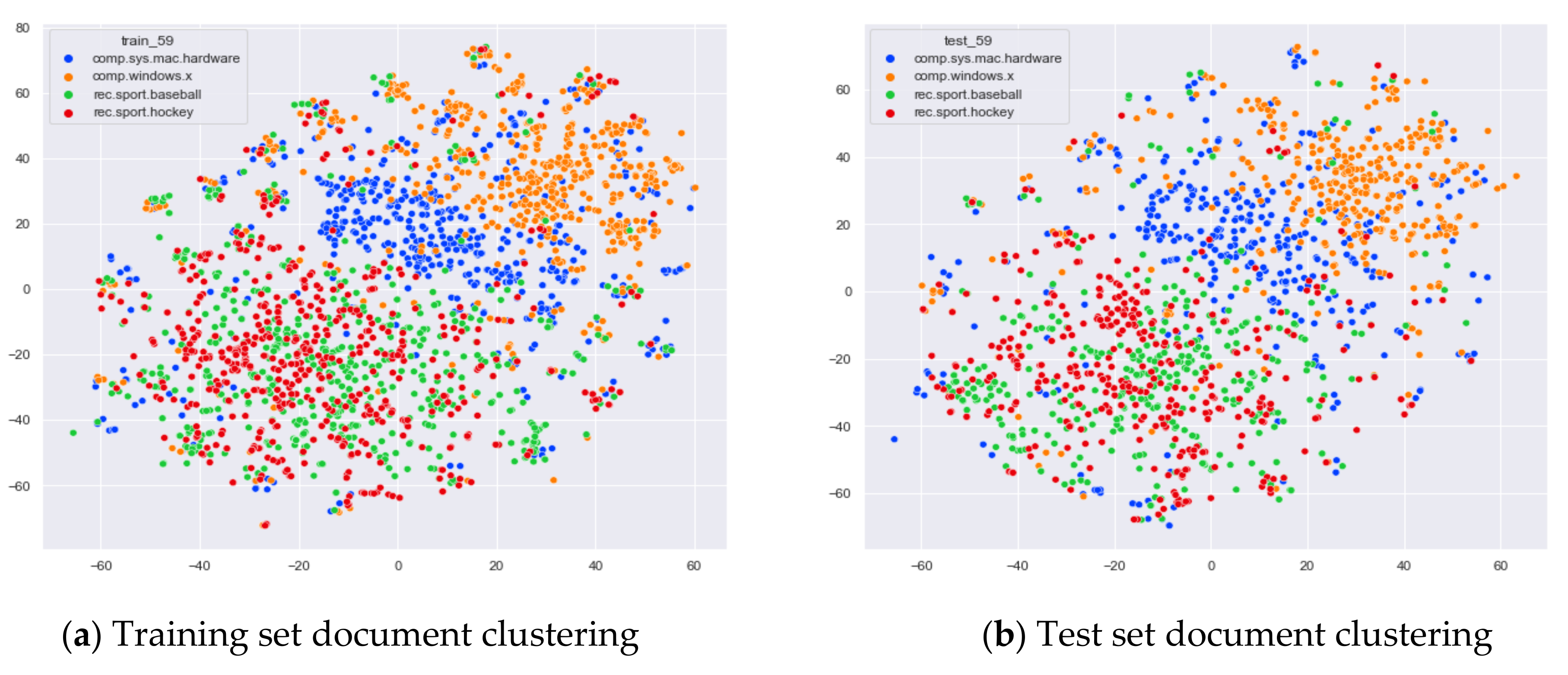
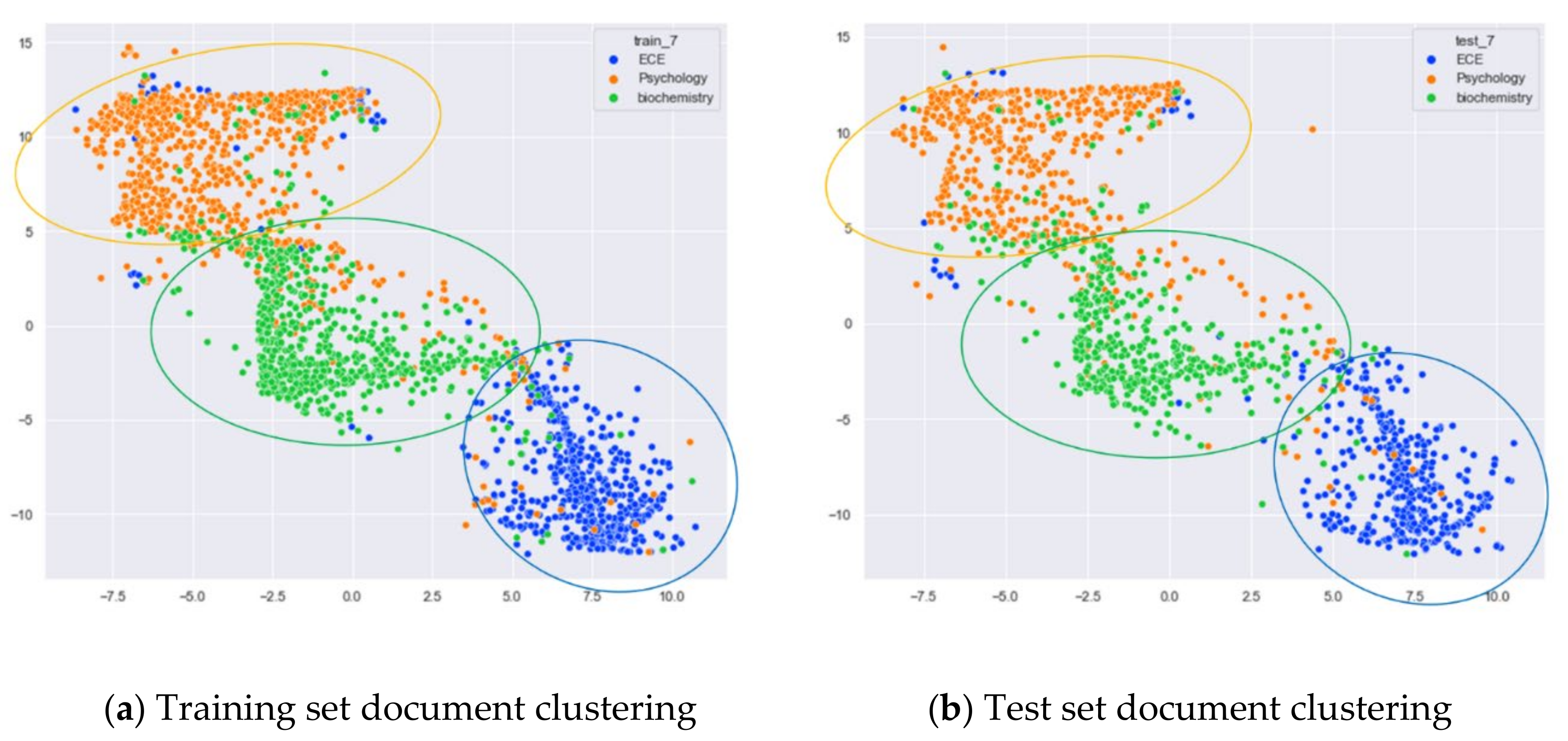
Clustering Effect Comparison
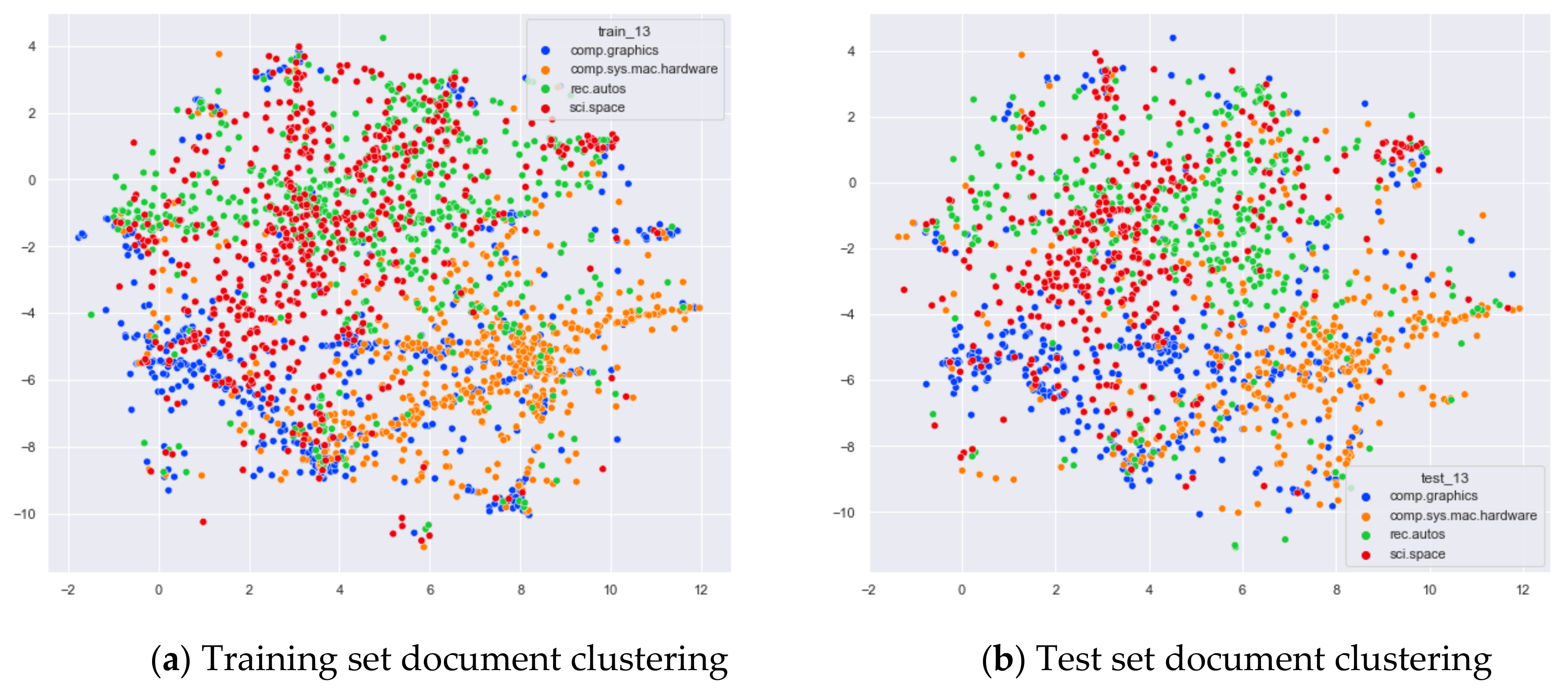
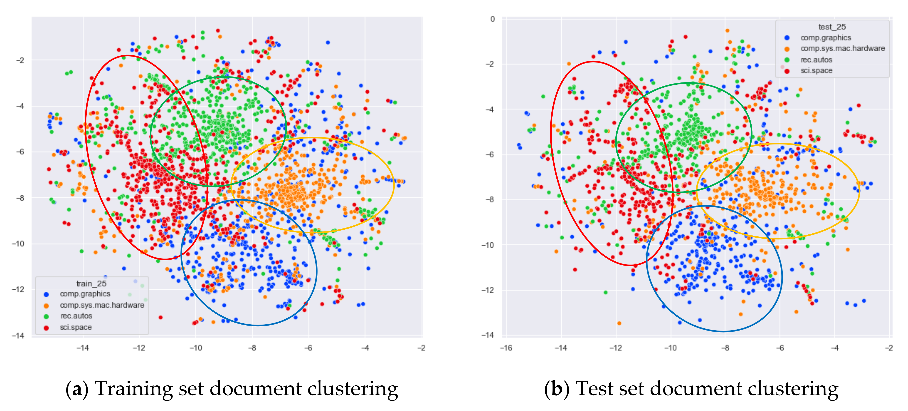
4.3.2. The Experimental Results of WOS_46986
Comparison of Different Topics Number Selection Methods
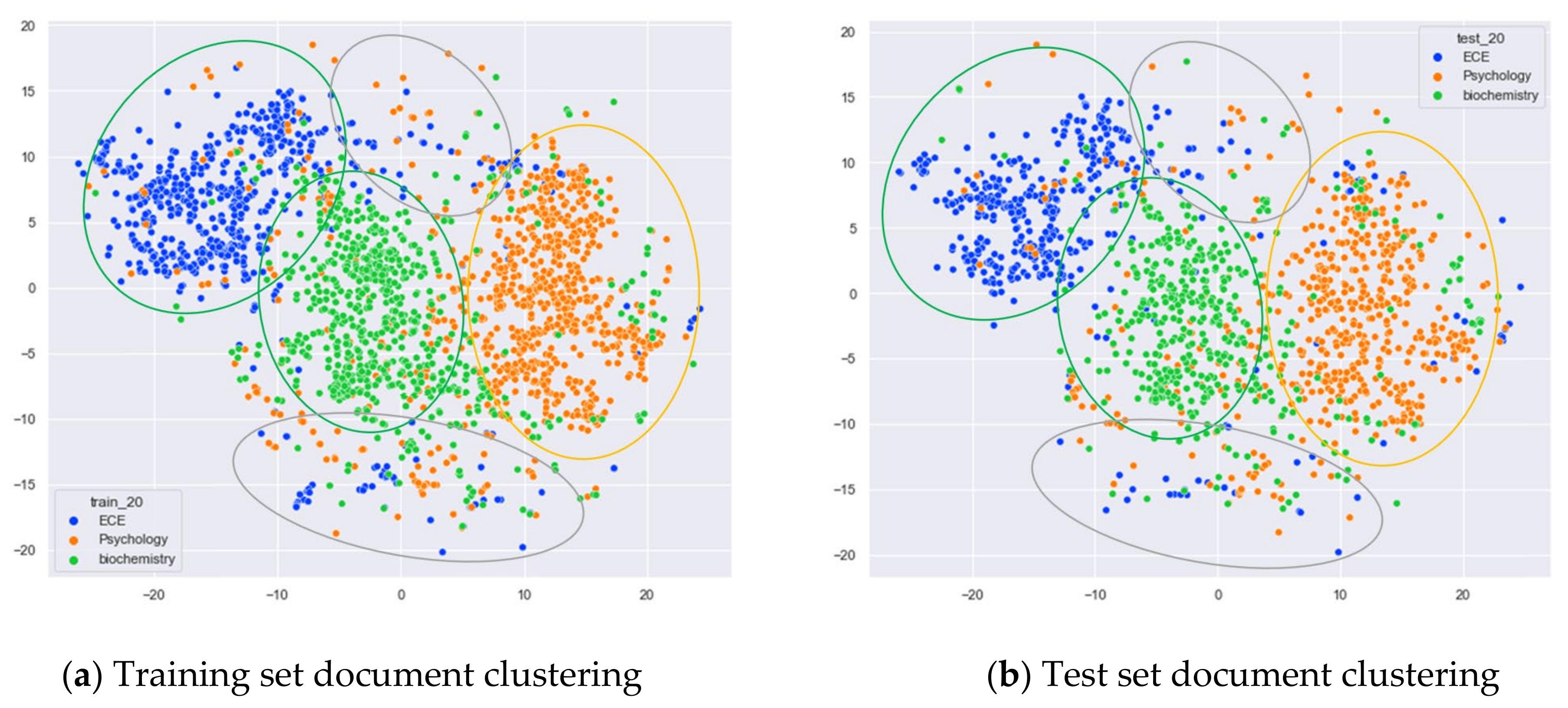
Clustering Effect Comparison
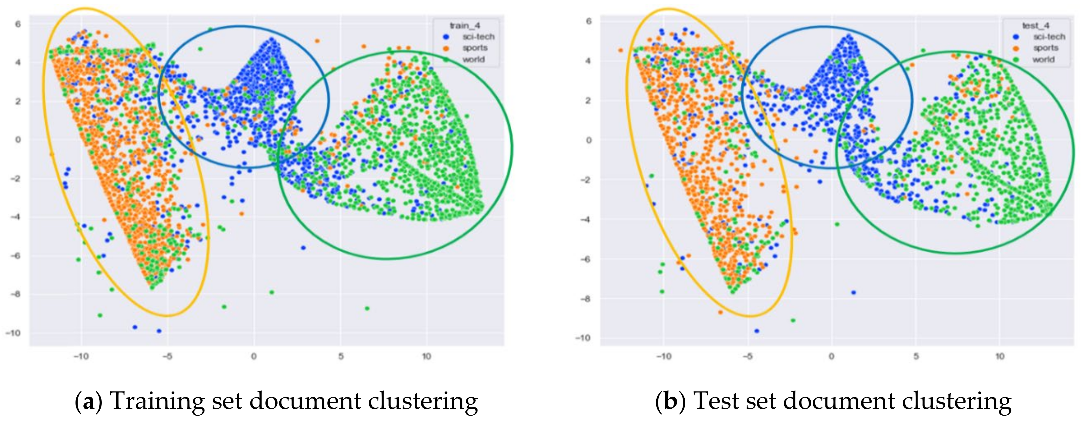
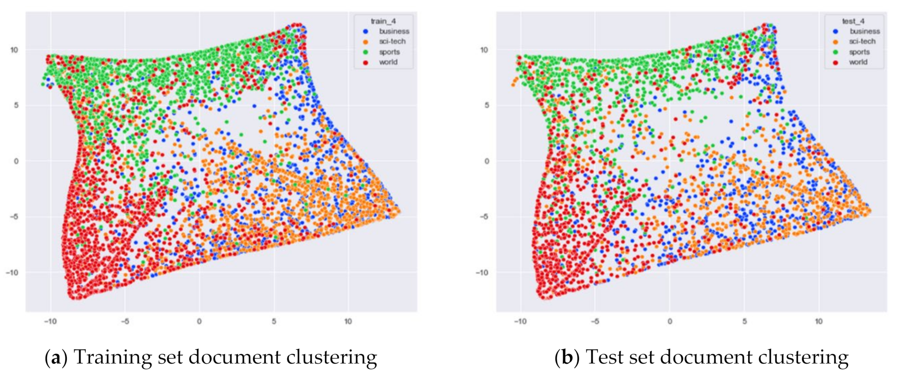
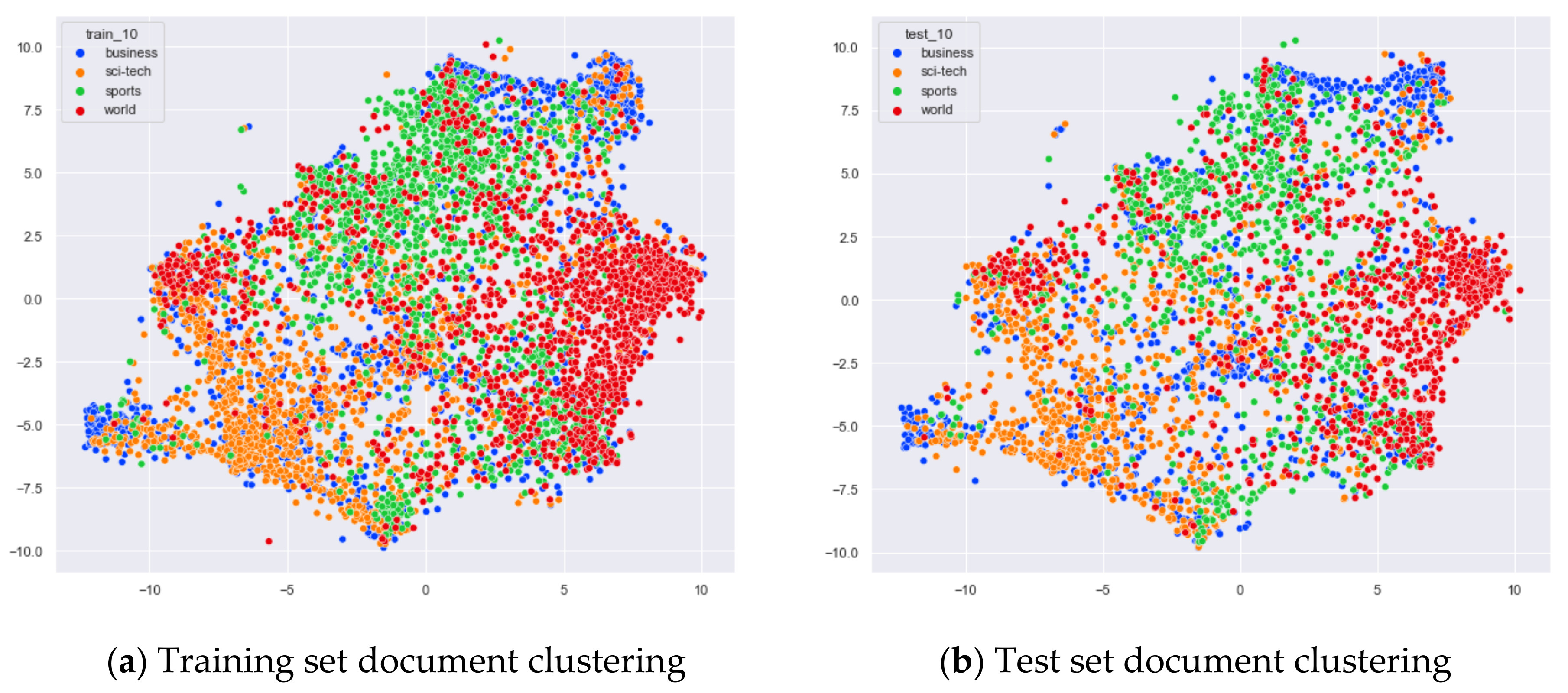
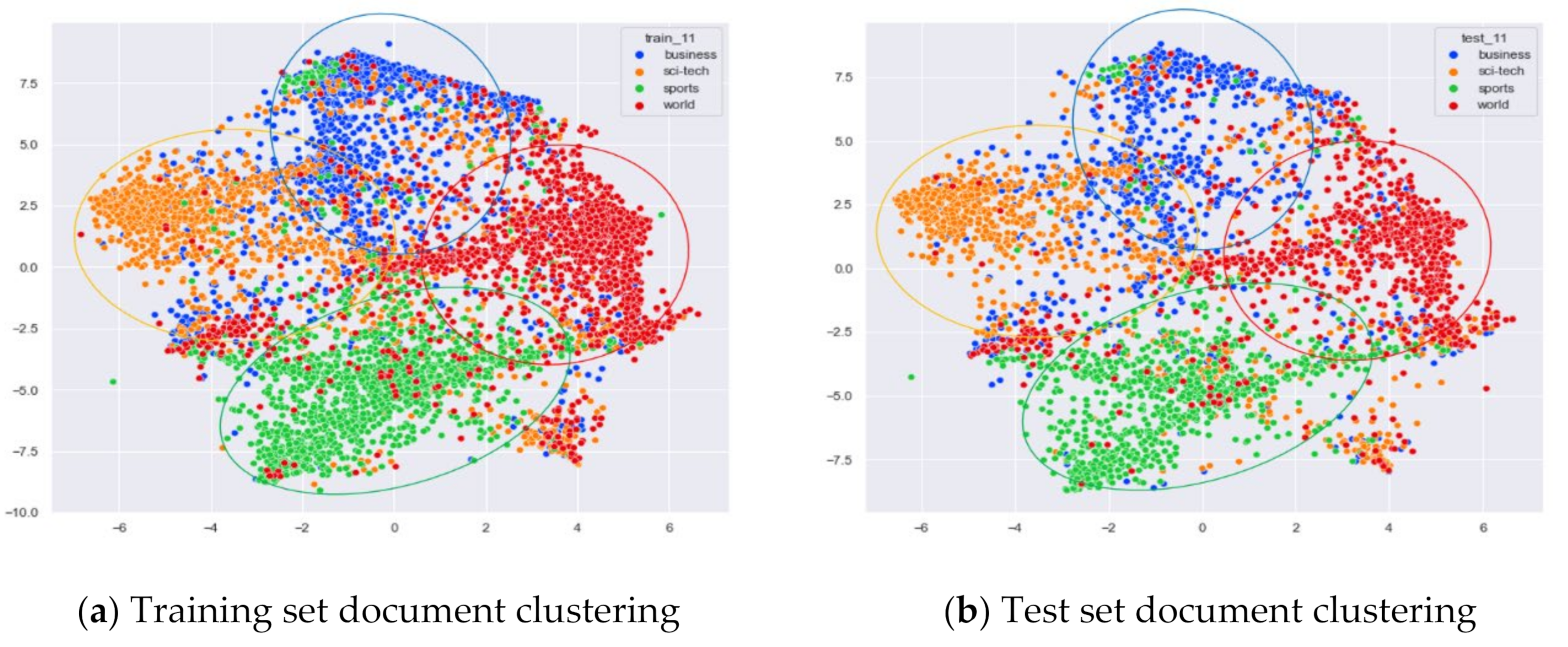
4.3.3. The Experimental Results of AG_News
Comparison of Different Topics Number Selection Methods
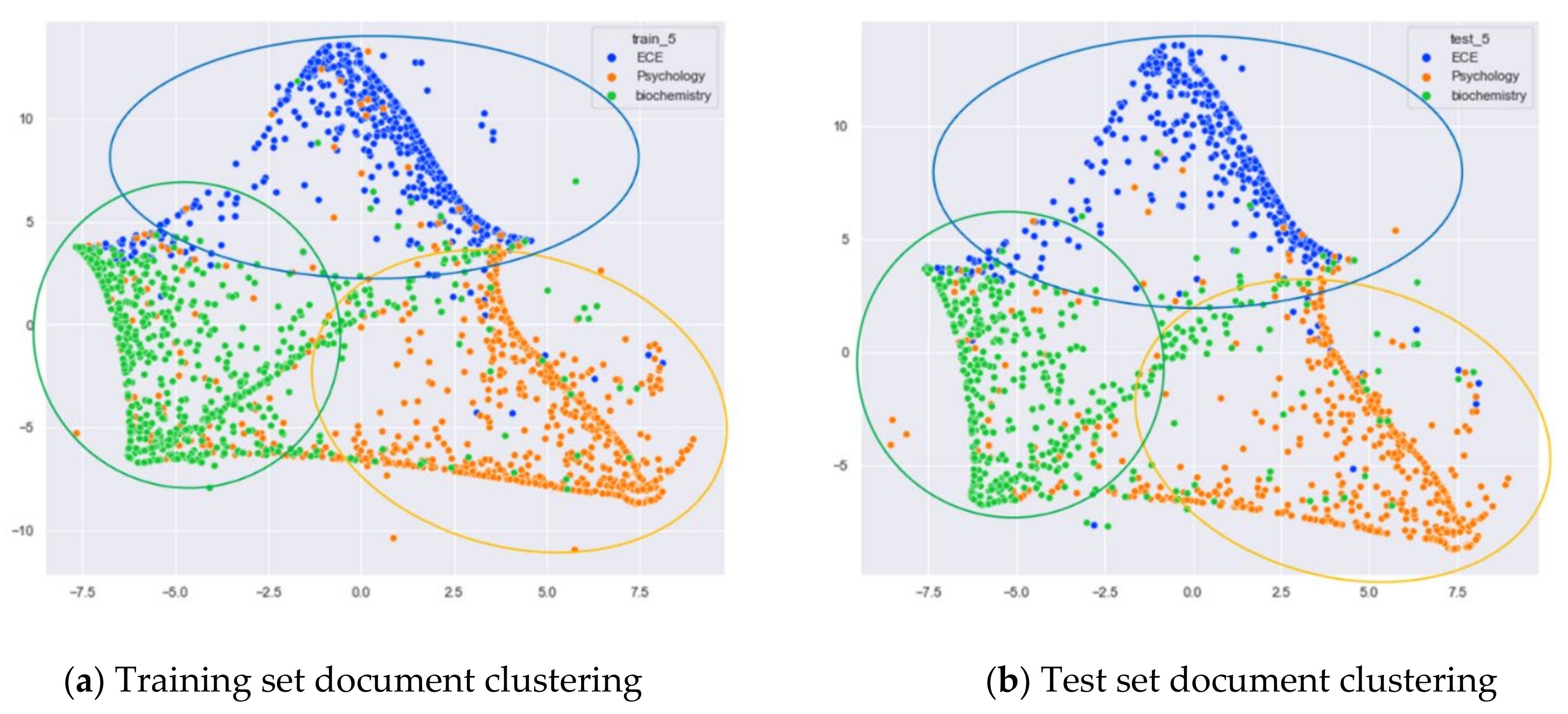
Clustering Effect Comparison
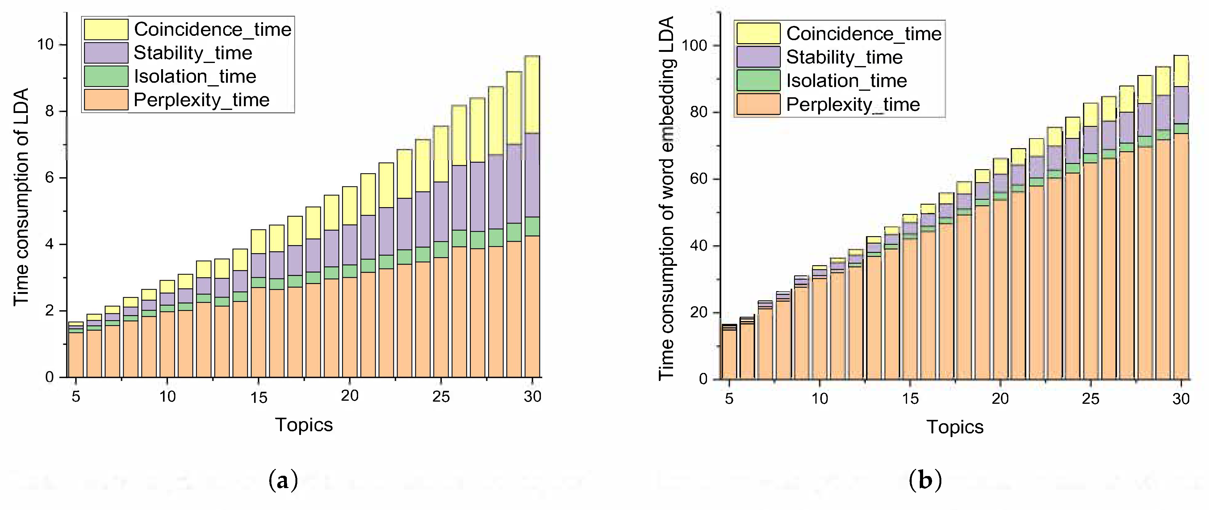
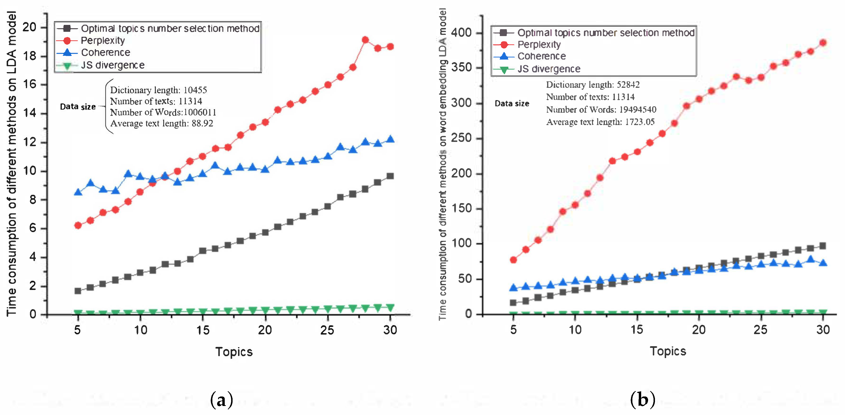
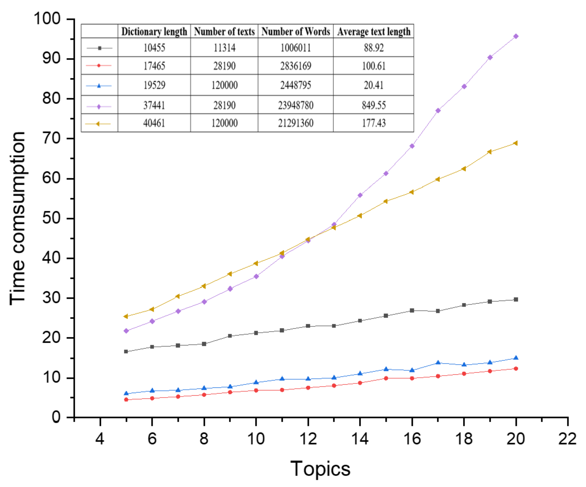
4.4. Comparison of Time Consumption
5. Experiment and Analysis for Real Data
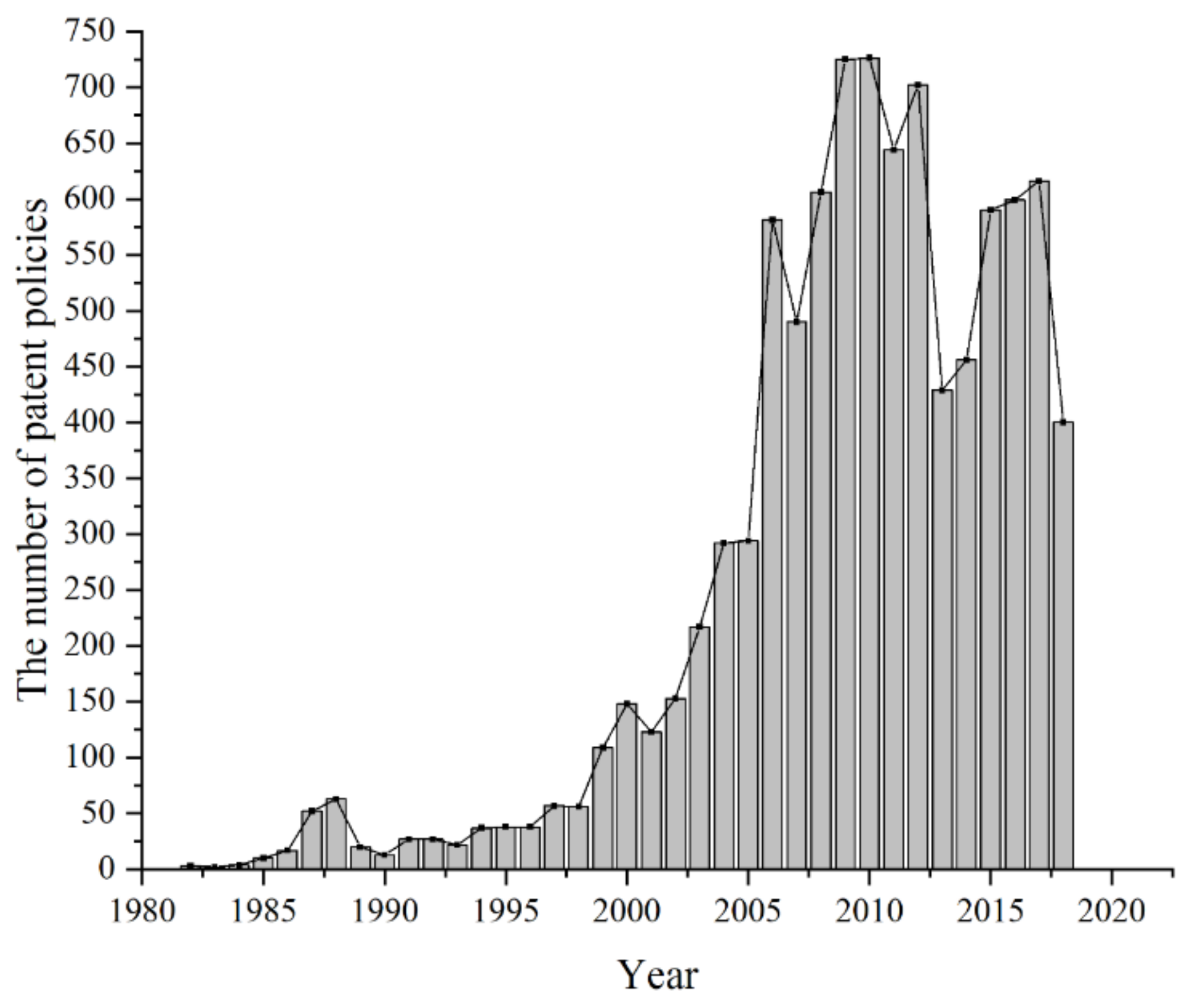
5.1. Data and Pre-Processing
5.2. LDA Model Training
5.3. Experimental Results and Comparative Analysis
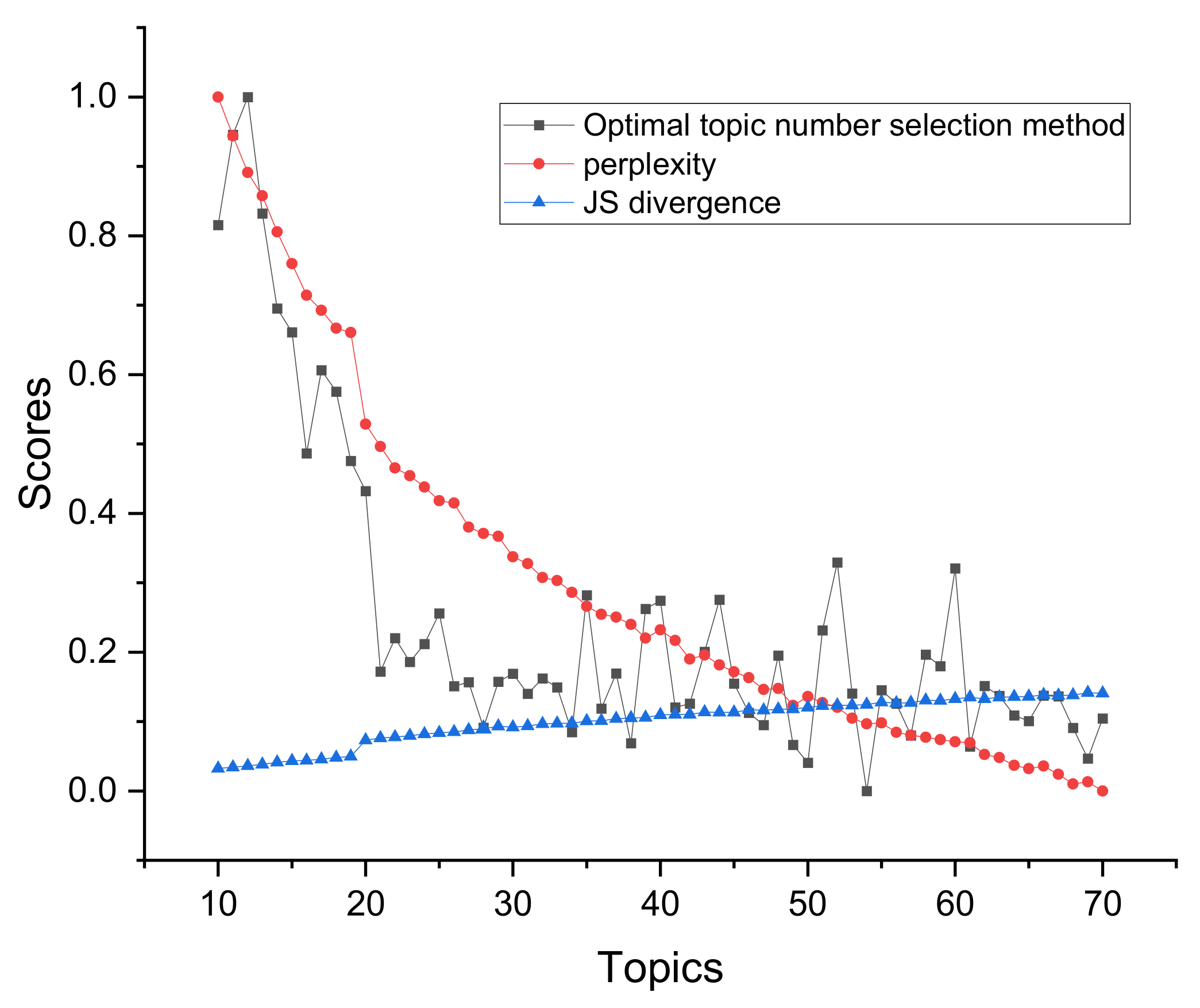
5.3.1. Comparison of Optimal Number of Topics
5.3.2. Comparison of Experimental Results
- (1)
- Patent creation policies. The management of patent-creating activities is an important function of the State Intellectual Property Office (SIPO), i.e., the examination and granting of patent rights. The target of the patent creation policy is mainly the creators of patents, including enterprises, research institutes, universities, and individual inventors. There are four main aspects of the patent creation policy: one is to encourage inventions and patent applications through awards and various prizes, the second is to encourage inventions and creations by means of title evaluation or high-tech evaluation, the third is to encourage the declaration of subject projects in key technical fields, and the fourth is the introduction of innovative talents.
- (2)
- Patent utilization policies. Patent utilization is a key step to realize the value of intellectual property rights (IPR). The current patent utilization policy focuses on promoting the industrialization and commercialization of patent achievements. Its policy targets are mainly the creators and users of patents.
- (3)
- Patent protection policies. Starting from 2014, many regional judicial systems in China have established dedicated IP courts for handling IP-related legal disputes. Meanwhile, special IPR actions conducted by the SIPO and local IPR bureaus as the leading units have also made progress in many aspects, strengthening the fight against IPR infringement through administrative protection means and further optimizing the IPR legal, market, and cultural environments. China’s IPR protection policy is currently facing many reforms, including enhancing the statutory means of IPR enforcement, optimizing IPR enforcement procedures, reforming comprehensive IPR administrative enforcement, and broadening IPR dispute resolution channels.
- (4)
- Patent management policies. The patent management policies are public policies that guide and regulate the IP management activities of power holders from the government level. They include upgrading the IP management level of patent rights holders, certification of IP consistent enterprises, management of project and personnel titles, etc. IP management activities are actions exercised by IPR subjects, and the policies are mainly guiding and encouraging policies, whose core objective is to enhance the IP management level of rights holders.
- (5)
- Patent service policies. Patent services are an important way to facilitate a good interface between patent creation, utilization, protection, and management. The content of patent service policies is encapsulated in the links of patent creation, utilization, protection, and management, and it transfers patent services originally provided by rights holders and government departments to third-party institutions in the market. A major shift in China’s current patent policy is to establish and improve the patent service industry system. Typical patent service businesses include public platforms for patent education and operation, patent information and intelligence, patent legal services, patent financial services, patent personnel training, and technology consulting. Promoting the formation of an industrial chain covering the whole process of patent creation, utilization, protection, and management in a competitive market environment is the main policy objective of patent service policy.
6. Conclusions and Discussion
Author Contributions
Funding
Institutional Review Board Statement
Informed Consent Statement
Data Availability Statement
Conflicts of Interest
References
- Greene, D.; O’Callaghan, D.; Cunningham, P. How Many Topics? Stability Analysis for Topic Models. Joint European Conference on Machine Learning and Knowledge Discovery in Databases; Springer: Berlin/Heidelberg, Germany, 2014. [Google Scholar]
- Zhang, P.; Wang, S.; Li, D.; Li, X.; Xu, Z. Combine topic modeling with semantic embedding: Embedding enhanced topic mode. IEEE Trans. Knowl. Data Eng. 2019, 32, 2322–2335. [Google Scholar] [CrossRef]
- Blei, D.M.; Ng, A.Y.; Jordan, M.I. Latent dirichlet allocation. J. Mach. Learn. Res. 2003, 3, 993–1022. [Google Scholar]
- Koltcov, S.; Ignatenko, V. Renormalization analysis of topic models. Entropy 2020, 22, 556. [Google Scholar] [CrossRef] [PubMed]
- Pavlinek, M.; Podgorelec, V. Text classification method based on self-training and LDA topic models. Expert Syst. Appl. 2017, 80, 83–93. [Google Scholar] [CrossRef]
- Kandemir, M.; Keke, T.; Yeniterzi, R. Supervising topic models with Gaussian processes. Pattern Recognit. 2018, 77, 226–236. [Google Scholar] [CrossRef]
- Guan, P.; Wang, Y.F. Identifying optimal topic numbers from Sci-Tech information with LDA model. Data Anal. Knowl. Discov. 2016, 9, 42–50. [Google Scholar]
- Maier, D.; Waldherr, A.; Miltner, P.; Wiedemann, G.; Niekler, A.; Keinert, A.; Pfetsch, B.; Heyer, G.; Reber, U.; Häussler, T. Applying LDA topic modeling in communication research: Toward a valid and reliable methodology. Commun. Methods Meas. 2018, 12, 93–118. [Google Scholar] [CrossRef]
- Chen, W.; Lin, C.R.; Li, J.Q.; Yang, Z.L. Analysis of the evolutionary trend of technical topics in patents based on LDA and HMM: Taking marine diesel engine technology as an example. J. China Soc. Sci. Tech. Inf. 2018, 37, 732–741. [Google Scholar]
- Liu, J.W.; Yang, B.; Wang, F.F.; Xu, S. Research on knowledge inheritance of academic pedigree based on LDA topic model—A case study of genetics pedigree with the core of Tan Jiazhen. Libr. Inf. Serv. 2018, 62, 76–84. [Google Scholar]
- Zhang, T.; Ma, H.Q. Clustering policy texts based on LDA topic model. Data Anal. Knowl. Discov. 2018, 2, 59–65. [Google Scholar]
- Yin, H.F.; Wu, H.; Ma, Y.X.; Ji, F.Y. Technical topic analysis in patents based on LDA and strategic diagram by taking graphene technology as an example. J. Intell. 2018, 37, 97–102. [Google Scholar]
- Zhang, H.; Xu, S.; Qiao, X.D. Review on topic models integrating intra- and extra-features of scientific and technical literature. J. China Soc. Sci. Tech. Inf. 2014, 10, 1108–1120. [Google Scholar]
- Bai, Z.A.; Zeng, J.P. Optimal selection method for LDA topics based on degree of overlap and completeness. Comput. Eng. Appl. 2019, 55, 155–161. [Google Scholar]
- Campos, L.; Fernández-Luna, J.; Huete, J.F.; Redondo-Expósito, L. LDA-based term profiles for expert finding in a political setting. J. Intell. Inf. Syst. 2021, 56, 1–31. [Google Scholar] [CrossRef]
- Sbalchiero, S.; Eder, M. Topic modeling, long texts and the best number of topics. Some Problems and solutions. Qual. Quant. 2020, 54, 1095–1108. [Google Scholar]
- Arun, R.; Suresh, V.; Madhavan, C.V.; Murthy, M.N. On Finding the Natural Number of Topics with Latent Dirichlet Allocation: Some Observations. Pacific-Asia Conference on Knowledge Discovery and Data Mining; Springer: Berlin/Heidelberg, Germany, 2010. [Google Scholar]
- He, J.Y.; Chen, X.S.; Du, M.; Jiang, H. Topic evolution analysis based on improved online LDA model. J. Cent. South Univ. Sci. Technol. 2015, 46, 547–553. [Google Scholar]
- Röder, M.; Both, A.; Hinneburg, A. Exploring the Space of Topic Coherence Measures. In Proceedings of the Eighth ACM International Conference on Web Search and Data Mining, Shanghai, China, 2–6 February 2015; Association for Computing Machinery: Shanghai, China, 2015; pp. 399–408. [Google Scholar]
- Lange, T.; Roth, V.; Braun, M.L.; Buhmann, J.M. Stability-based validation of clustering solutions. Neural Comput. 2004, 16, 1299–1323. [Google Scholar] [CrossRef] [PubMed]
- 20 Newsgroups. Available online: http://qwone.com/~jason/20Newsgroups/ (accessed on 23 August 2021).
- Mendeley Data. Available online: https://data.mendeley.com/datasets/9rw3vkcfy4/ (accessed on 10 September 2021).
- AG’s Corpus of News Articles. Available online: http://groups.di.unipi.it/~gulli/AG_corpus_of_news_articles.html (accessed on 10 September 2021).
- LemmInflect. Available online: https://pypi.org/project/lemminflect/ (accessed on 23 August 2021).
- Gensim 4.1.2. Available online: https://pypi.org/project/gensim/ (accessed on 23 August 2021).
- Hagen, L. Content analysis of e-petitions with topic modeling: How to train and evaluate LDA models? Inf. Process. Manag. 2018, 54, 1292–1307. [Google Scholar] [CrossRef]
- Teh, Y.W.; Jordan, M.I.; Beal, M.J.; Blei, D.M. Hierarchical Dirichlet Processes. J. Am. Stat. Assoc. 2006, 101, 1566–1581. [Google Scholar] [CrossRef]
- Pennington, J.; Socher, R.; Manning, C.D. Glove: Global Vectors for Word Representation. In Proceedings of the Conference on Empirical Methods in Natural Language Processing, Doha, Qatar, 25–29 October 2014. [Google Scholar]
- Module Tomotopy. Available online: https://bab2min.github.io/tomotopy/v0.4.1/en/ (accessed on 23 August 2021).
- TSNE. Available online: https://scikit-learn.org/stable/modules/generated/sklearn.manifold.TSNE.html (accessed on 23 August 2021).
- Jieba 0.42.1. Available online: https://pypi.org/project/jieba/ (accessed on 23 August 2021).
- Das, R.; Zaheer, M.; Dyer, C. Gaussian LDA for Topic Models with Word Embeddings. In Proceedings of the 53rd Annual Meeting of the Association for Computational Linguistics and the 7th International Joint Conference on Natural Language Processing (Volume 1: Long Papers), Beijing, China, 26–31 July 2015. [Google Scholar]
- Pan, Y.; Jian, Y.; Liu, S.; Jing, L. A Biterm-based Dirichlet Process Topic Model for Short Texts. In Proceedings of the 3rd International Conference on Computer Science and Service System, Bangkok, Thailand, 13–15 June 2014. [Google Scholar]


| Topics | “Topic-Word” Probability | Topic Content |
|---|---|---|
| 2 | Topic1{‘apple’: 0.37895802, ‘pear’: 0.29479387, ‘dog’: 0.21694316, ‘pig’: 0.06072744, ‘cat’: 0.048577495} | Fruits |
| Topic2{‘dog’: 0.42677134, ‘cat’: 0.23052387, ‘pig’: 0.21749169, ‘apple’: 0.06457374, ‘pear’: 0.060639422} | Animals | |
| 3 | Topic1{‘apple’: 0.40487534, ‘pear’: 0.31113106, ‘dog’: 0.21715428, ‘pig’: 0.034434676, ‘cat’: 0.03240472} | Fruits |
| Topic2{‘dog’: 0.4494548, ‘cat’: 0.24006312, ‘pig’: 0.23640023, ‘apple’: 0.037318606, ‘pear’: 0.03676326} | Animals | |
| Topic3{‘dog’: 0.21185784, ‘pig’: 0.2001333, ‘apple’: 0.19875155, ‘pear’: 0.196671, ‘cat’: 0.19258636} | Animals | |
| 4 | Topic1{‘apple’: 0.3716775, ‘dog’: 0.23012395, ‘pear’: 0.22663262, ‘pig’: 0.08662834, ‘cat’: 0.084937565} | Unknown |
| Topic2{‘dog’: 0.4598837, ‘cat’: 0.24295807, ‘pig’: 0.24179693, ‘apple’: 0.02782605, ‘pear’: 0.027535275} | Animals | |
| Topic3{‘dog’: 0.20344584, ‘apple’: 0.20050451, ‘pig’: 0.20007579, ‘pear’: 0.19842108, ‘cat’: 0.19755279} | Unknown | |
| Topic4{‘apple’: 0.39690995, ‘pear’: 0.33073652, ‘dog’: 0.2127626, ‘pig’: 0.029939024, ‘cat’: 0.029651856} | Fruits |
| Test Documents | Number of Topics = 2 | Number of Topics = 3 | Number of Topics = 4 |
|---|---|---|---|
| Test1 | P(Topic1|Test1) = 0.6808042 P(Topic2|Test1) = 0.3191958 | P(Topic1|Test1) = 0.59324664 P(Topic2|Test1) = 0.31827474 P(Topic3|Test1) = 0.08847858 | P(Topic1|Test1) = 0.06545124 P(Topic2|Test1) = 0.30757654 P(Topic3|Test1) = 0.06323278 P(Topic4|Test1) = 0.56373950 |
| Test2 | P(Topic1|Test2) = 0.18206072 P(Topic2|Test2) = 0.81793930 | P(Topic1|Test2) = 0.11509656 P(Topic2|Test2) = 0.77113570 P(Topic3|Test2) = 0.11376770 | P(Topic1|Test2) = 0.08417302 P(Topic2|Test2) = 0.74760187 P(Topic3|Test2) = 0.08373206 P(Topic4|Test2) = 0.08449302 |
| Topics | Perplexity | JS | Coherence | Stability | Coincidence | Optimal Topic Number Selection Method |
|---|---|---|---|---|---|---|
| 2 | 2.2899 | 0.0471 | 0.8536 | 0.9630 | 2 | 100.9598 |
| 3 | 2.2567 | 0.0601 | 0.8047 | 0.9620 | 3 | 117.0119 |
| 4 | 2.2526 | 0.0637 | 0.7803 | 0.9623 | 4 | 147.0472 |
| d | AJ | |||
|---|---|---|---|---|
| 1 | Results | Technology | 0 | 0 |
| 2 | Results, Translation | Technology, Contracts | 0 | 0 |
| 3 | Results, Translation, Technology | Technology, Contracts, Market | 0.200 | 0.067 |
| 4 | Results, Translation, Technology, Market | Technology, Contracts, Market, Regulations | 0.333 | 0.133 |
| 5 | Results, Translation, Technology, Market, Contracts | Technology, Contracts, Market, Regulations, Management | 0.429 | 0.193 |
| sim20 | sim50 | sim80 | sim100 | Mean | |
|---|---|---|---|---|---|
| sim20 | - | 0.9949 | 0.9917 | 0.9901 | 0.9922 |
| sim50 | 0.9949 | - | 0.999 | 0.9982 | 0.9974 |
| sim80 | 0.9917 | 0.999 | - | 0.9998 | 0.996833 |
| sim100 | 0.9901 | 0.9982 | 0.9998 | - | 0.9960 |
| Dataset | 20news_groups | WOS_46986 | AG_news | |||||||||
| Model | LDA | word_embedding | LDA | word_embedding | LDA | word_embedding | ||||||
| Data size | 100% | 80% | 100% | 80% | 100% | 80% | 100% | 80% | 100% | 80% | 100% | 80% |
| Dictionary length | 10,455 | 10,455 | 52,842 | 52,842 | 17,465 | 17,465 | 37,441 | 37,441 | 19,529 | 19,529 | 40,461 | 40,461 |
| Number of texts | 11314 | 9051 | 11314 | 9051 | 28,190 | 22,552 | 28,190 | 22,552 | 120,000 | 96,000 | 120,000 | 96,000 |
| Bag of Words | 1,006,011 | 803,520 | 19,494,540 | 15,752,120 | 2,836,169 | 2,428,971 | 23,948,780 | 19,199,000 | 2,448,795 | 1,960,293 | 21,291,360 | 17,042,060 |
| Average text length | 88.92 | 88.78 | 1723.05 | 1740.37 | 100.61 | 107.71 | 849.55 | 851.32 | 20.41 | 20.42 | 177.43 | 177.52 |
| sim20 | sim50 | sim80 | sim100 | Mean | |
|---|---|---|---|---|---|
| sim20 | - | 0.9697 | 0.9362 | 0.9195 | 0.9418 |
| sim50 | 0.9697 | - | 0.9917 | 0.9839 | 0.981767 |
| sim80 | 0.9362 | 0.9917 | - | 0.9986 | 0.9755 |
| sim100 | 0.9195 | 0.9839 | 0.9986 | - | 0.967333 |
| Topic | word1 | prob1 | word2 | prob2 | word3 | prob3 | word4 | prob4 | word5 | prob5 |
|---|---|---|---|---|---|---|---|---|---|---|
| 0 | enterprise | 0.1175 | center | 0.0885 | technology | 0.0669 | recognition | 0.0199 | R&D | 0.0194 |
| word6 | prob6 | word7 | prob7 | word8 | prob8 | word9 | prob9 | word10 | prob10 | |
| research | 0.0191 | engineering | 0.0177 | evaluation | 0.0139 | technology innovation | 0.0135 | development | 0.0127 | |
| 1 | word1 | prob1 | word2 | prob2 | word3 | prob3 | word4 | prob4 | word5 | prob5 |
| activity | 0.1292 | propaganda | 0.0388 | popularization of science | 0.0372 | organization | 0.0296 | science | 0.0253 | |
| word6 | prob6 | word7 | prob7 | word8 | prob8 | word9 | prob9 | word10 | prob10 | |
| innovation | 0.0212 | hold | 0.0201 | unit | 0.0169 | junior | 0.0145 | science | 0.0131 | |
| 2 | word1 | prob1 | word2 | prob2 | word3 | prob3 | word4 | prob4 | word5 | prob5 |
| project | 0.0910 | capital | 0.0774 | special funds | 0.0316 | management | 0.0298 | use | 0.0269 | |
| word6 | prob6 | word7 | prob7 | word8 | prob8 | word9 | prob9 | word10 | prob10 | |
| unit | 0.0226 | method | 0.0183 | subsidy | 0.0165 | finance | 0.0129 | funds | 0.0123 | |
| 3 | word1 | prob1 | word2 | prob2 | word3 | prob3 | word4 | prob4 | word5 | prob5 |
| enterprise | 0.1126 | reward | 0.0503 | science | 0.0315 | subsidy | 0.0279 | exceed | 0.0259 | |
| word6 | prob6 | word7 | prob7 | word8 | prob8 | word9 | prob9 | word10 | prob10 | |
| support | 0.0241 | highest | 0.0202 | capital | 0.0195 | subsidy | 0.0194 | disposable | 0.0191 | |
| 4 | word1 | prob1 | word2 | prob2 | word3 | prob3 | word4 | prob4 | word5 | prob5 |
| export | 0.0786 | trade | 0.0634 | product | 0.0447 | technology | 0.0403 | machining | 0.0347 | |
| word6 | prob6 | word7 | prob7 | word8 | prob8 | word9 | prob9 | word10 | prob10 | |
| enterprise | 0.0306 | identify | 0.0292 | international | 0.0252 | cooperation | 0.0203 | introduce | 0.0181 |
| Topic | word1 | prob1 | word2 | prob2 | word3 | prob3 | word4 | prob4 | word5 | prob5 |
|---|---|---|---|---|---|---|---|---|---|---|
| 0 | enterprise | 0.0982 | privately operated | 0.0893 | science | 0.0338 | institution | 0.0300 | regulation | 0.0228 |
| word6 | prob6 | word7 | prob7 | word8 | prob8 | word9 | prob9 | word10 | prob10 | |
| management | 0.0198 | private technology | 0.0159 | science staff | 0.0140 | operation | 0.0136 | technology | 0.0117 | |
| 1 | word1 | prob1 | word2 | prob2 | word3 | prob3 | word4 | prob4 | word5 | prob5 |
| goal achievement | 0.1685 | announcement | 0.1332 | project department | 0.0467 | industrialization and urbanization | 0.0000 | expand | 0.0000 | |
| word6 | prob6 | word7 | prob7 | word8 | prob8 | word9 | prob9 | word10 | prob10 | |
| profession | 0.0000 | specialization | 0.0000 | patent | 0.0000 | patent technology | 0.0000 | patent application | 0.0000 | |
| 2 | word1 | prob1 | word2 | prob2 | word3 | prob3 | word4 | prob4 | word5 | prob5 |
| science | 0.0596 | innovation | 0.0531 | technology | 0.0260 | enterprise | 0.0250 | autonomy | 0.0169 | |
| word6 | prob6 | word7 | prob7 | word8 | prob8 | word9 | prob9 | word10 | prob10 | |
| highlights | 0.0168 | high technology | 0.0151 | innovation ability | 0.0120 | research | 0.0118 | major | 0.0115 | |
| 3 | word1 | prob1 | word2 | prob2 | word3 | prob3 | word4 | prob4 | word5 | prob5 |
| handle | 0.0339 | management | 0.0305 | request | 0.0278 | dispute | 0.0274 | office | 0.0183 | |
| word6 | prob6 | word7 | prob7 | word8 | prob8 | word9 | prob9 | word10 | prob10 | |
| party | 0.0174 | complaint | 0.0153 | secrecy | 0.0152 | license | 0.0143 | regulation | 0.0139 | |
| 4 | word1 | prob1 | word2 | prob2 | word3 | prob3 | word4 | prob4 | word5 | prob5 |
| patent | 0.4377 | implementation | 0.0343 | patent technology | 0.0304 | institution | 0.0278 | agent | 0.0268 | |
| word6 | prob6 | word7 | prob7 | word8 | prob8 | word9 | prob9 | word10 | prob10 | |
| patent application | 0.0240 | patent right | 0.0224 | management | 0.0209 | invention | 0.0126 | proxy | 0.0092 |
| Optimal topic Number Selection Method | Number of Fuzzy Topics | Precision (P) | Recall (R) | F-Value | Fuzzy Rate | ||||
|---|---|---|---|---|---|---|---|---|---|
| JS divergence | 70 | 52 | 55 | 1 | 17 | 74.29% | 94.55% | 83.20% | 24.29% |
| Perplexity | 70 | 52 | 55 | 1 | 17 | 74.29% | 94.55% | 83.20% | 24.29% |
| Topic superiority index | 54 | 49 | 55 | 0 | 5 | 90.74% | 89.09% | 89.91% | 9.26% |
| Optimal Topic Number Selection Method | Number of Patent Creation Policies | Number of Patent Utilization Policies | Number of Patent Protection Policies | Number of Patent Management Policies | Number of Patent Service Policies | Precision (P) | Recall (R) | F-Value | |||
|---|---|---|---|---|---|---|---|---|---|---|---|
| JS divergence | 13 | 5 | 5 | 16 | 4 | 8 | 18 | 16 | 38.46% | 100.00% | 55.56% |
| Perplexity | 13 | 5 | 5 | 16 | 4 | 8 | 18 | 16 | 38.46% | 100.00% | 55.56% |
| Topic superiority index | 5 | 5 | 5 | 14 | 4 | 6 | 17 | 13 | 100.00% | 100.00% | 100.00% |
| Patent Policy Category | Subclass | Topic |
|---|---|---|
| Patent creation policies | Reward and subsidy | Topic 3 Technology awards and subsidies; Topic 16 Patent application funding |
| Encouraging technology R&D | Topic 9 Encouraging innovation investment; Topic 12 Encouraging technology R&D; Topic 17 Encouraging autonomy innovation | |
| Subsidies for technological innovation in various fields | Topic 6 Declaration for medical projects; Topic 24 Innovation of agroforestry; Topic 28 High-performance technology creation; Topic 29 Development of key technologies in various fields; Topic 46 Industrial information technology upgrading; Topic 51 Energy-saving and environmental protection projects; Topic 53 Development of high-tech industry | |
| Competition awards | Topic 35 Publicity of awards for projects of various organizations; Topic 37 Innovation competition | |
| Patent utilization policies | Trade | Topic 4 Import and export trade |
| Tax reduction | Topic 7 Tax reduction for the utilization of technical products | |
| Technology utilization | Topic 23 Technology utilization and promotion | |
| Achievement transformation | Topic 31 Awards for transformation of scientific and technological achievements | |
| Patent protection policies | Contract guarantee | Topic 14 Technology transfer contract; Topic 22 Technology trade contract |
| Infringement dispute | Topic 43 Patent related disputes; Topic 44 Infringement and anti-counterfeiting; Topic 47 IP protection action; Topic 48 Administrative law enforcement | |
| Patent management policies | Special management | Topic 0 Technology identification and evaluation management; Topic 2 Management of the special fund |
| Project management | Topic 8 Project acceptance management; Topic 10 Project planning; Topic 32 Project declaration management; Topic 33 Project award management | |
| Title management | Topic 5 Achievement identification of technical title; Topic 18 Technical personnel qualification audit management | |
| System management | Topic 21 System reform and management; Topic 27 Economic performance appraisal management; Topic 8 Management of administrative units; Topic 42 System reform and economic performance | |
| Enterprise management | Topic 19 High-tech declaration management; Topic 25 Standardization management; Topic 30 Improvement of comprehensive capability of IP; Topic 45 Model enterprise of IP management; Topic 49 Technology management of private enterprises | |
| Patent service policies | Science education and talent | Topic 1 Popular science propaganda; Topic 26 Technology services; Topic 34 Education training; Topic 38 Introduction of technical talents |
| Service industry | Topic 11 Capacity improvement of service industry; Topic 41 Agent institute; Topic 52 Finance services | |
| Platform service | Topic 13 Technology transformation platform; Topic 15 Product exhibition; Topic 36 Information platform; Topic 39 Industrial integration platform | |
| Incubation base | Topic 20 Entrepreneurship and innovation incubation base; Topic 50 Technology development zone |
Publisher’s Note: MDPI stays neutral with regard to jurisdictional claims in published maps and institutional affiliations. |
© 2021 by the authors. Licensee MDPI, Basel, Switzerland. This article is an open access article distributed under the terms and conditions of the Creative Commons Attribution (CC BY) license (https://creativecommons.org/licenses/by/4.0/).
Share and Cite
Gan, J.; Qi, Y. Selection of the Optimal Number of Topics for LDA Topic Model—Taking Patent Policy Analysis as an Example. Entropy 2021, 23, 1301. https://doi.org/10.3390/e23101301
Gan J, Qi Y. Selection of the Optimal Number of Topics for LDA Topic Model—Taking Patent Policy Analysis as an Example. Entropy. 2021; 23(10):1301. https://doi.org/10.3390/e23101301
Chicago/Turabian StyleGan, Jingxian, and Yong Qi. 2021. "Selection of the Optimal Number of Topics for LDA Topic Model—Taking Patent Policy Analysis as an Example" Entropy 23, no. 10: 1301. https://doi.org/10.3390/e23101301
APA StyleGan, J., & Qi, Y. (2021). Selection of the Optimal Number of Topics for LDA Topic Model—Taking Patent Policy Analysis as an Example. Entropy, 23(10), 1301. https://doi.org/10.3390/e23101301