Abstract
In this article, we introduce a new three-parameter distribution called the extended inverse-Gompertz (EIGo) distribution. The implementation of three parameters provides a good reconstruction for some applications. The EIGo distribution can be seen as an extension of the inverted exponential, inverse Gompertz, and generalized inverted exponential distributions. Its failure rate function has an upside-down bathtub shape. Various statistical and reliability properties of the EIGo distribution are discussed. The model parameters are estimated by the maximum-likelihood and Bayesian methods under Type-II censored samples, where the parameters are explained using gamma priors. The performance of the proposed approaches is examined using simulation results. Finally, two real-life engineering data sets are analyzed to illustrate the applicability of the EIGo distribution, showing that it provides better fits than competing inverted models such as inverse-Gompertz, inverse-Weibull, inverse-gamma, generalized inverse-Weibull, exponentiated inverted-Weibull, generalized inverted half-logistic, inverted-Kumaraswamy, inverted Nadarajah–Haghighi, and alpha-power inverse-Weibull distributions.
1. Introduction
The two-parameter Gompertz (Go) distribution is very important in modeling actuarial tables and human mortality. It was, historically, introduced by [1], after which many authors have contributed to its statistical methodology and characterization. Several studies have shown that the Go distribution is not flexible for modeling various phenomena due to it having only an increasing hazard rate (HR) shape, for example, the generalized-Go [2], beta-Go [3], transmuted-Go [4], McDonald-Go [5], exponentiated generalized Weibull-Go [6], unit-Go [7], power-Go [8], skew reflected-Go [9], Topp-Leone Go [10], and alpha-power Go [11] distributions.
Furthermore, Wu et al. [12] estimated the parameters of the Go distribution using the least-squares approach. Soliman et al. [13] estimated the parameters of the Go distribution using the maximum likelihood (ML) and Bayes methods under progressive first-failure censored samples. Dey et al. [14] studied the properties and different methods of estimation for the Go distribution.
Recently, many authors have constructed inverted models and studied their applications in several applied fields such as the inverse Nakagami-m, inverse weighted-Lindley, and logarithmic transformed inverse-Weibull distributions by [15,16,17], respectively.
Eliwa et al. [18] proposed the two-parameter inverse Go (IGo) distribution with an upside-down bathtub shape HR function. The non-negative random variable () X is said to have an IGo distribution if its cumulative distribution function (CDF) is specified (for ) by
where and denote the shape and scale parameters, respectively.
The first objective of this article is to present a new lifetime model called the EIGo distribution and explore some of its useful properties. Specifically, the EIGo model is constructed based on the extended-R (E-R) family [19] by adding another shape parameter that might address the lack of fit of the IGo distribution for modeling real-life data that indicated non-monotone failure rates. We are motivated to construct the EIGo distribution because (i) it is capable of modelling unimodal HR shape, which provides a good fit for the real data sets; (ii) the EIGo model contains some special well-known distributions; (iii) the EIGo model can be considered as a good alternative to the IGo model and other competing inverted models for fitting the positive data with a longer right tail; and (iv) the EIGo distribution outperforms some competing inverted distributions with respect to two real engineering data sets. One of the important advantages of the EIGo model is its ability to provide an improved fit with respect to its competing inverted models.
The second objective is to address and evaluate the behavior of classical and Bayesian estimators for the unknown parameters of the proposed EIGo distribution under Type-II censored samples. We compare the performances of these estimators by conducting extensive simulations in terms of their root mean squared errors (RMSEs) and relative absolute biases (RABs).
The paper is outlined in seven sections. In Section 2, the EIGo distribution is introduced with its special cases and expansion. Some of its useful properties are addressed in Section 3. In Section 4, maximum likelihood and Bayesian methods are discussed under Type-II censored samples. In Section 5, the performances of the maximum likelihood and Bayesian approaches are explored via simulation results. In Section 6, the adaptability of the EIGo model is addressed using two real-life engineering datasets. Finally, some concluding remarks are presented in Section 7.
2. The EIGo Distribution
In this section, we introduce the three-parameter EIGo distribution and some of its sub-models. The CDF of the E-R family, with a shape parameter , has the form
A lifetime X is said to have the EIGo distribution if its CDF has the form
where and denote the shape parameters and denotes the scale parameter. The first advantage of the EIGo distribution is that it has a closed form for its CDF (3).
The corresponding probability density function (PDF) of (3) becomes
The with the PDF (4) is denoted by EIGo. The EIGo distribution involves three well-known lifetime sub-models as follows.
- The generalized inverted-exponential (GIE) distribution [20] follows when the parameter .
- The IGo distribution [18] is derived for .
- The inverse-exponential (IE) distribution [21] with one parameter can be derived when and .
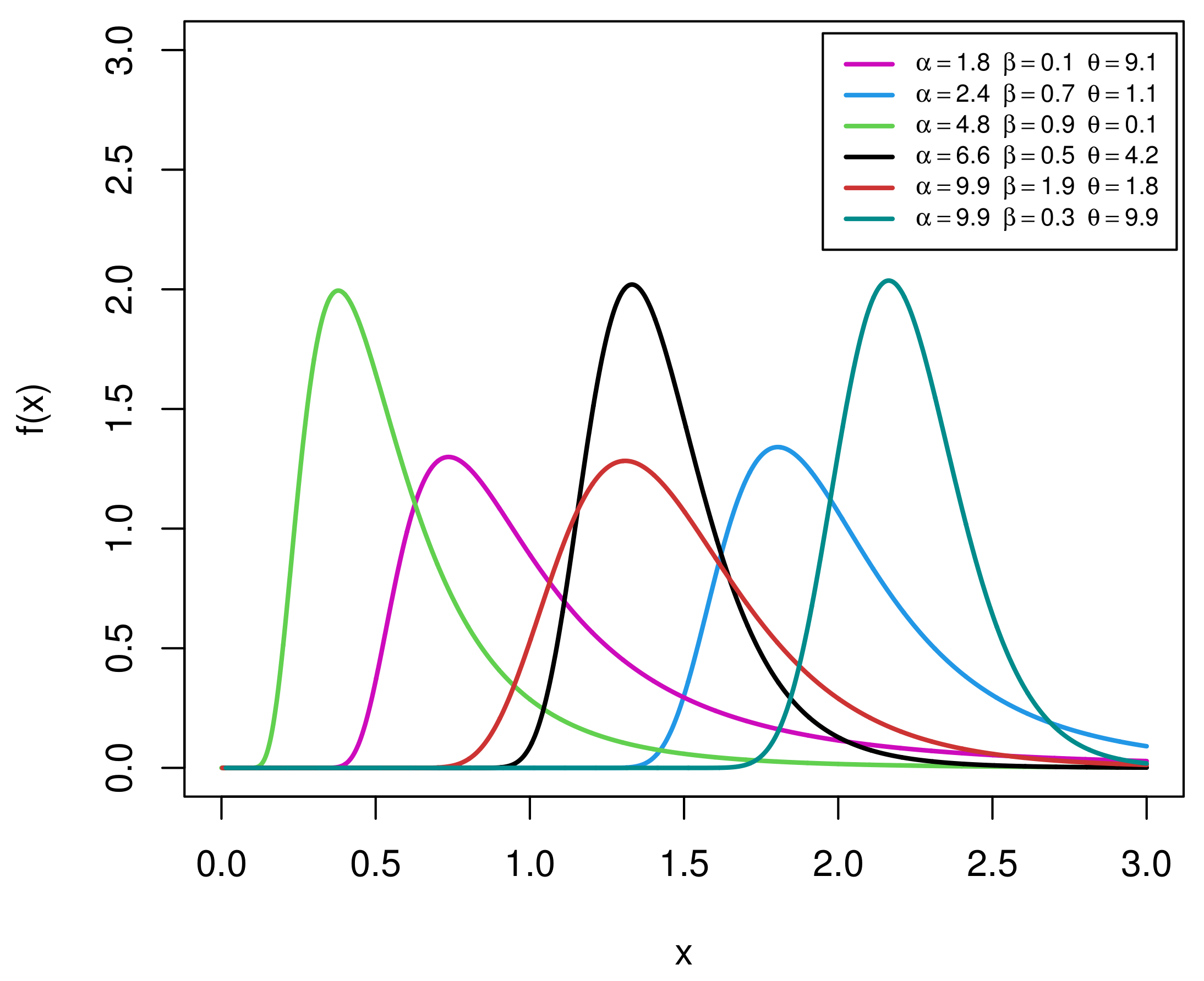
Using some specific parameter values, the shapes of the EIGo PDF (4) are displayed in Figure 1. It shows that the PDF of the EIGo distribution can be unimodal and right-skewed with great heaviness of the tails.
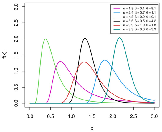
Figure 1.
Plots of the PDF of the EIGo distribution for some specific parameter values.
The corresponding survival, , and HR, , functions of the EIGo distribution have the forms
and
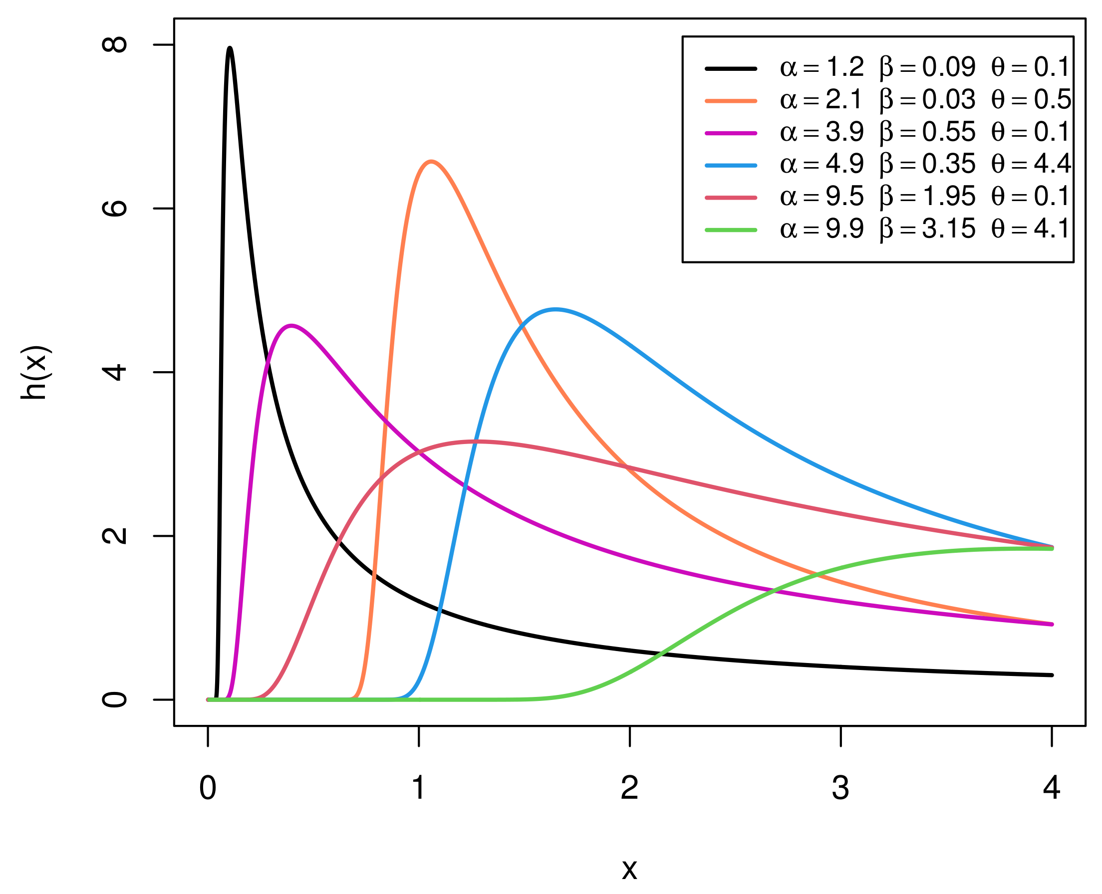
Figure 2 provides graphical representations of the HR function (HRF) of the EIGo distribution with various values of its parameters. It shows that the HRF of the EIGo distribution has an upside-down bathtub shape.
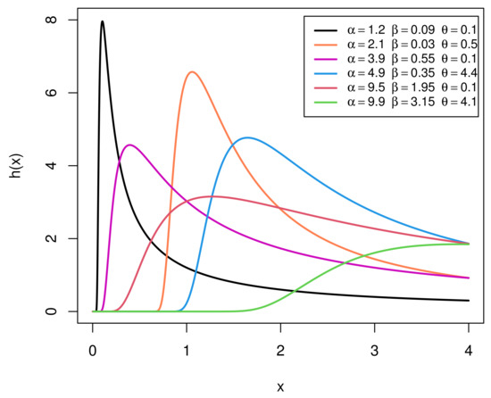
Figure 2.
Plots of the HRF of the EIGo distribution for some specific parameter values.
The cumulative HRF, , of the EIGo distribution has the form
The reversed HRF, of the EIGo distribution is
Expansions
Let a be a real positive integer; we consider the following general binomial series
which is valid for . By expanding the CDF (3) by (7), we get
where is the CDF of the IGo distribution with parameters and , and the coefficient is given by
Similarly, expanding the PDF (4) by (7), we obtain
where is the PDF of the IGo model with parameters and , and .
Clearly, Equation (9) shows that the EIGo model is a linear combination of IGo densities. Thus, some structural properties of the EIGo model can be obtained from those of the IGo distribution.
3. Statistical and Reliability Characteristics
This section is devoted to determining several statistical and reliability characteristics of the EIGo distribution.
3.1. Quantile and Mode
To simulate random samples from the EIGo distribution, its quantile function (QF), , follows as
Substituting into (10), the median, , of the EIGo distribution can conveniently be derived. Similarly, substituting and into (10), the first and the third quartiles of the EIGo distribution can be easily obtained.
The mode of the EIGo distribution follows by differentiating the logarithm of the PDF (4), , with respect to x, and equating the result to zero. After some algebraic manipulations, the mode is determined by solving the following non-linear equation:
The unique mode of the EIGo distribution cannot be obtained analytically, hence it can be obtained numerically.
3.2. Mean Residual Life
The mean-residual-life (MRL) function is the average remaining life span, which is a component surviving up to distinct time t. It is a useful measure in reliability studies for describing the aging process.
Theorem 1.
If X has EIGo distribution, thus the MRL of the lifetime X, say , takes the form
3.3. Mean Inactivity Time
The mean inactivity time (MIT) function is useful in reliability and survival analysis. The MIT, , of X is defined as
If EIGo, then, using (8), we have
3.4. Strong MIT
The strong-MIT (SMIT) function is another useful reliability measure, which is introduced by [23]. They showed that the SMIT has several properties that can be adopted in different applications in reliability and survival analysis. It can be used to predict the actual time at which the failure of the component or device occurs.
The SMIT, , has the form
Hence, the SMIT of the EIGo distribution follows as
3.5. Stress–Strength Reliability
The stress–strength model describes the life of a component or system that has a random strength X that may fail because it is subjected to a random stress Z. Hence, is a measure of component reliability.
Suppose X and Z have independent EIGo and EIGo with the same shape parameter . Then, the stress–strength measure is [24]
3.6. Probability Weighted Moments
The probability-weighted moments (PWM), say , can be adopted to derive an estimate for the unknown parameters of a particular distribution whose inverse extension cannot be expressed explicitly.
Theorem 2.
If X has EIGo distribution, then the PWM of the X is derived as
3.7. Moments
Moments are used to describe the characteristics of the probability distribution, so they are important in any statistical analysis.
By definition, the r-th moment of any X with PDF, , is
By substituting (9) in (25), the rth moment of the EIGo distribution reduces to
where
is the gamma (Ga) function.
From (26), the corresponding mean of the EIGo distribution is simply obtained by setting , and the corresponding variance can be also obtained using and .
3.8. Entropies
Entropy is a useful concept to measure the uncertainty related to a X. It is adopted in many fields of science such as econometrics and computer science.
The Rényi entropy of order , say , is defined (for and ) as [26]
So, if EIGo distribution, then we have
where
Hence, the of X becomes
The -entropy, denoted by , of the EIGo distribution has the form (for and )
It follows directly using (27).
3.9. Order Statistics
Consider the order statistics (OS) of a random sample of size n, say . Then, the PDF of the order statistic, say is [27]
where .
The corresponding CDF of reduces to
3.10. Stochastic Ordering
The following theorem shows that the EIGo distribution is ordered with respect to the likelihood ratio, , order.
Theorem 3.
Let EIGo and EIGo, for , then .
4. Parameter Estimation under Type-II Censoring
In this section, we discuss the estimation of the EIGo parameters, , using the ML and Bayesian estimators under Type-II censoring scheme in which the life-test is terminated after a specified number of failures have occurred, say , out of complete test units n.
4.1. Maximum Likelihood Estimators
Suppose that n independent items are taken from the EIGo model with CDF (3) and are placed on a test at time 0. Hence, the likelihood function (LF), say , under Type-II censored sample, , takes the form (See [29])
By substituting (3) and (4) into (34), then Equation (34) reduces to
where and . Clearly, the LF of complete sample follows as a special case from (35) by setting . The associated log-LF of (35), say , becomes
Differentiating (36) partially with respect to , and , we can write that the log-LF of (35), say , becomes
and
where is the first-partial derivative with respect to , , , , and .
Equating the three Equations (37)–(39) to zero and solving them simultaneously will provide the ML estimators (MLEs) of the EIGo parameters. Clearly, the MLEs cannot be determined in closed forms, but they can be calculated numerically using suitable iterative techniques such as the Newton–Raphson. To construct the confidence intervals (CIs) of the model parameters, the observed information matrix, , is required, and it takes the form
Practically, by dropping the expectation operator given in (40) and replacing by their MLEs , the approximate asymptotic variance–covariance matrix, , for the MLEs , becomes
Taking the second partial derivative of (36) with respect to , , and , the observed Fisher elements in (41), , are obtained and are available with the authors upon request. Under some mild regularity conditions, the MLEs are approximately distributed as multivariate normal (No) distribution with mean and variance respectively [29]. Hence, for large samples, CIs for the model parameters and are
respectively, where , , and refer to diagonal elements of (41) and is the percentile of the standard No distribution with right-tail probability -th.
4.2. Bayes Estimators
This subsection discusses the Bayes estimators (BEs) and the credible intervals (CIs) of the unknown parameters of the EIGo model. The squared error loss (SEL) function as a symmetric loss function is adopted to obtain the BEs, and it is defined by
where is an estimate of .
The gamma (Ga) conjugate priors of the EIGo parameters can be applied to develop the BEs due to their flexibility in covering several varieties of prior beliefs of the experimenter (see [30,31]). Hence, the unknown parameters , and are assumed to have independent Ga prior PDF, i.e., as Ga, Ga and Ga. The hyper-parameters, say , represent the prior knowledge about the three parameters, and they are assumed to be non-negative and known. However, the hyper-parameters are fixed by using the mean and the variance of the Ga distribution ( and ); hence, is used and is the initial value. Hence, the joint prior PDF of becomes
Combining (43) with (35), the joint posterior distribution of , and becomes
where
and refers to the normalizing constant of (44).
Then, the BEs of any function of , , and , say , under the SEL function follows by the posterior expectation of , and it has the form
Based on (45), the BEs cannot be obtained in closed forms. Hence, the Markov chain Monte Carlo (MCMC) techniques are adopted to approximate the BEs and to construct the CIs from (45). The Metropolis Hastings (M-H) algorithm is a general technique of a family of Markov chain (MC) simulation methods, and it is the most commonly used of MCMC techniques to draw samples from posterior distribution (PD) to calculate the Bayesian estimates of interest. Several applications of the MC algorithm can be explored in [31,32].
Thus, from (46), the unknown parameter has the Ga density with shape parameter and scale parameter . Thus, the samples of are generated easily using any Ga-generating routine. In addition, from (47) and (48), it can be seen that the CPDs of and are different from well-known distributions. Hence, it is impossible to sample directly using standard models. To solve this problem, Tierney [33] proposed the use of a hybrid MCMC algorithm by combining the M-H algorithm sampler with a Gibbs sampling scheme using the normal distribution. Here, the hybrid algorithm will be termed as a M-H within Gibbs sampling for updating the unknown parameter using Gibbs steps and then for updating the unknown parameters and using M-H steps in order to calculate the BEs and construct the CIs of , , and . Now, the proposed hybrid algorithm can be carried out using the following steps.
Step 1: Start with an initial values , , and .
Step 2: Set .
Step 3: Generate from .
Step 4: Generate and from and using M-H algorithm with the normal densities:
(a) Generate and from and , respectively.
(b) Obtain the acceptance measures:
and
.
(c) Generate samples and from .
(d) If then set . Similarly if then set . Otherwise set and .
Step 5: Put .
Step 6: Repeat steps 3-5 for M times to get
In the beginning of the analysis (burn-in period), we discarded the first simulated varieties, say , to remove the effect of the selection of initial guess value and to guarantee the sampling convergence; hence, the remaining samples are used to carried out the BEs with an optimal acceptance rate of 23.4% [34]. Then, for sufficiently large M, the drawn MCMC samples of the parameters , , and as in , can be adopted to develop the BEs. Thus, the approximate BEs of under SEL function takes the form
To construct the two-sided Bayes-CIs (BCIs) of , , and , we order the simulated MCMC samples of for after burn-in as . Hence, the two-sided BCIs of reduces to
5. Simulation Results
To evaluate the behavior of the point and interval estimators for the EIGo parameters, we conduct a Monte Carlo simulation study. Using three sets of parametric values, i.e., , , and , we simulate 1000 samples of n (total sample size) and m (effective sample size) such as , 60, and 80, where m is taken as a failure proportion such as 50, 75, and 100% for each n. Clearly, the Type-II censored samples, which are generated with , represent the complete samples. In the Bayesian paradigm, the choice of the hyper-parameter value is a crucial issue. Therefore, if the proper prior information (PI) is available for , , and i.e., , then the joint posterior distribution (44) is proportional to the likelihood function (35). Hence, if one does not have PI on the unknown parameters, it is better to adopt the MLEs instead of the BEs because the latter are very expensive computationally.
Here, we adopted two informative priors for each set of , , and , called prior (1): ; prior (2): when as well as prior (1): ; prior (2): when . Here, the values of hyper parameters of , , and are determined in such a way that the prior mean becomes the expected value of the estimated parameter [30]. The hybrid MCMC algorithm described in Section 4.2 is adopted to generate 12,000 MCMC samples, and we discarded the first 2000 values as ‘burn-in’. Accordingly, the average Bayes MCMC estimates and 95% two-sided BCIs are calculated based on 10,000 MCMC samples.
For each setting, we compute the average estimates, , with their root mean squared errors (RMSEs) and RABs using the following formulae.
where N is the number of replicates, is an estimate of , , , and .
The required numerical results are performed using the software. The average values of , , and , RMSEs, and RABs are reported in Table 1, Table 2 and Table 3. In addition, the average confidence lengths (ACLs) of 95% asymptotic CIs of , , and are summarized in Table 4.

Table 1.
The average estimates of and their respective RMSEs and RABs in parentheses.
Table 2.
The average estimates of and their respective RMSEs and RABs in parentheses.
Table 3.
The average estimates of and their respective RMSEs and RABs in parentheses.
Table 4.
The ACLs for 95% ACIs/BCIs of , , and .
From Table 1, Table 2 and Table 3, it can be shown that the proposed estimates of the parameters , , and are very good in terms of minimum RMSEs and RABs. Further, as n or m increases, the performance of the estimates becomes better. Moreover, the point estimates become even better with the increase in failure-proportion . Finally, the Bayes MCMC estimates using Ga informative priors are better as they include prior information than the frequentist estimates in term of their RMSEs and RABs. Generally, we conclude that the BEs based on prior (2) performed better than those based on prior (1) in terms of minimum RABs, RMSEs, and ACLs. This is due to the fact that the variance of prior (2) is lower than the variance of prior (1), and both are more informative than an improper prior for .
Furthermore, the ACLs of asymptotic CIs are narrowed down with the increase in n and m. In addition, the CIs perform better than the asymptotic intervals due to the Ga prior information with respect to the shortest ACLs. Moreover, when the true values of , , and increase, it is clear that the associated RMSEs, RABs, and ACLs of all proposed estimates increase. Finally, we recommend the Bayesian MCMC estimation of the parameters of the EIGo distribution using the hybrid Gibbs within the M-H algorithm sampler.
6. Real-Life Applications
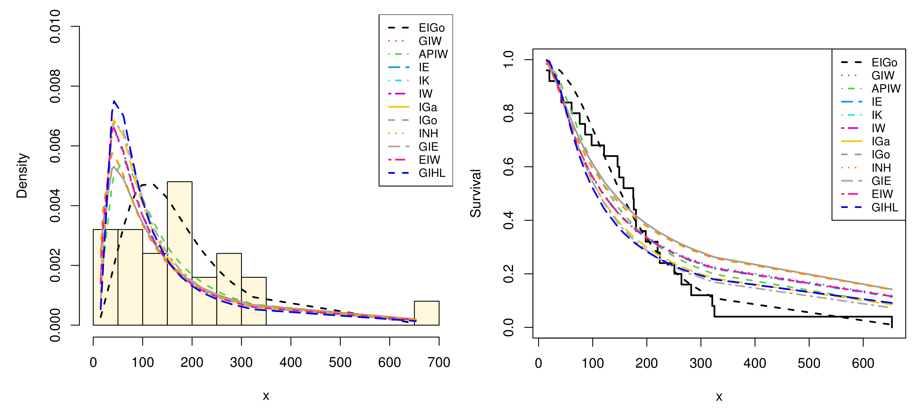
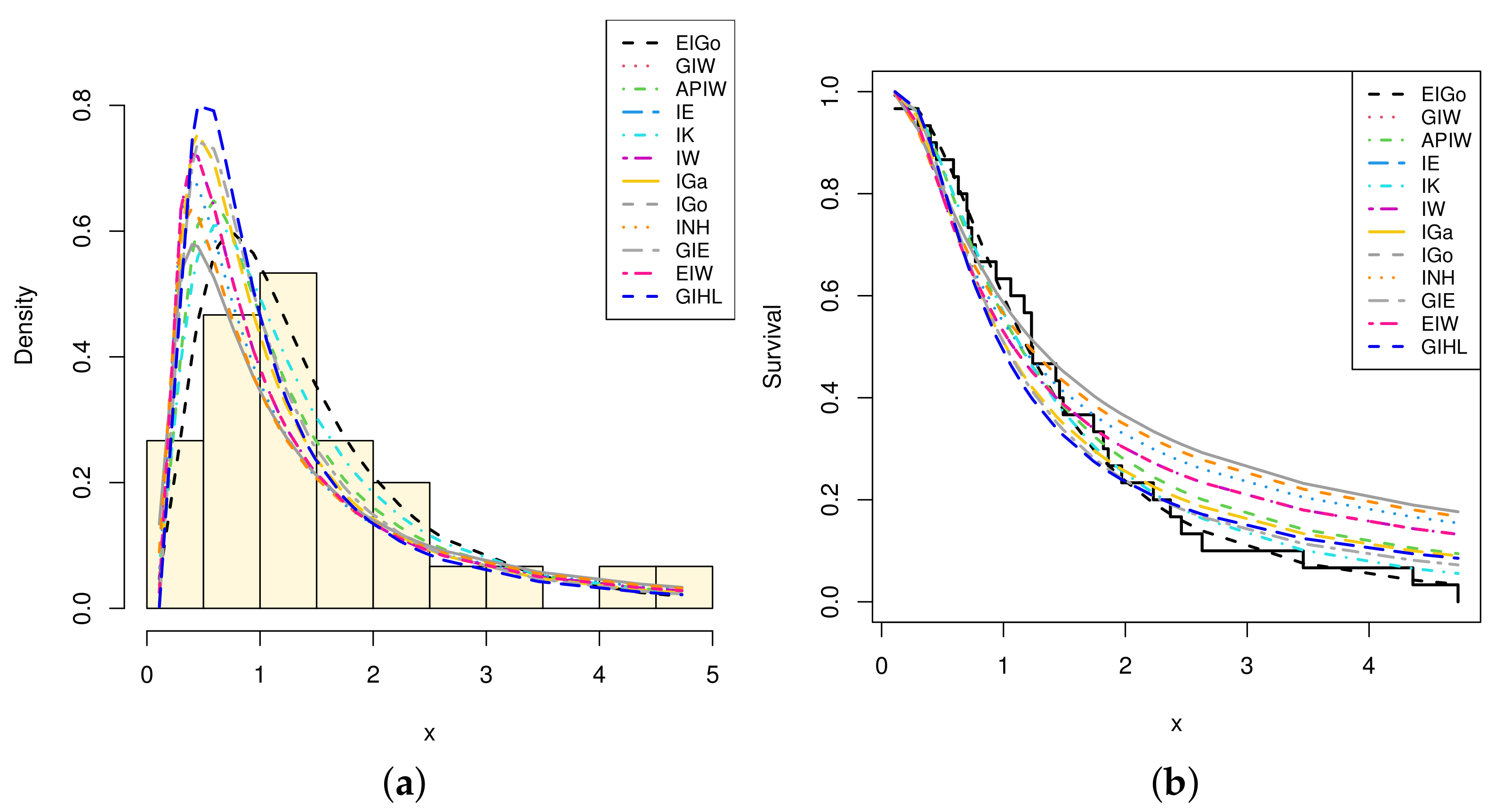
The importance and flexibility of the EIGo model are discussed empirically by analyzing two real data from engineering science. The first dataset consists of 25 (100 cm) specimens of yarn, which were tested at a certain strain level, and it represents the number of cycles to failure [29,35]. The data are: 20, 15, 61, 38, 98, 42, 86, 76, 146, 121, 157, 149, 175, 180, 176, 180, 220, 198, 224, 264, 251, 282, 325, 321, 653. The second dataset shows the time between failures for repairable mechanical equipment items [36]. The data are: 0.11, 0.30, 0.40, 0.45, 0.59, 0.63, 0.70, 0.71, 0.74, 0.77, 0.94, 1.06, 1.17, 1.23, 1.23, 1.24, 1.43, 1.46, 1.49, 1.74, 1.82, 1.86, 1.97, 2.23, 2.37, 2.46, 2.63, 3.46, 4.36, 4.73.
The EIGo distribution is compared with some competing distributions such as the IGo, IE [21], GIE [20], inverse-Weibull (IW) [37], inverse gamma (IGa) [38], generalized inverse-Weibull (GIW) [39], exponentiated inverted-Weibull (EIW) [40], generalized inverted half-logistic (GIHL) [41], inverted-Kumaraswamy (IK) [42], inverted Nadarajah–Haghighi (INH) [43], and alpha-power inverse-Weibull (APIW) [44] distributions. The corresponding PDFs of the competing models (for ) are written in Table 5.
Table 5.
Some competing inverted models of the EIGo distribution.
Moreover, to check the validity of the EIGo model along with other competing models, we employed several goodness-of-fit measures as listed in Table 6.
Table 6.
Some useful criteria for model selection.
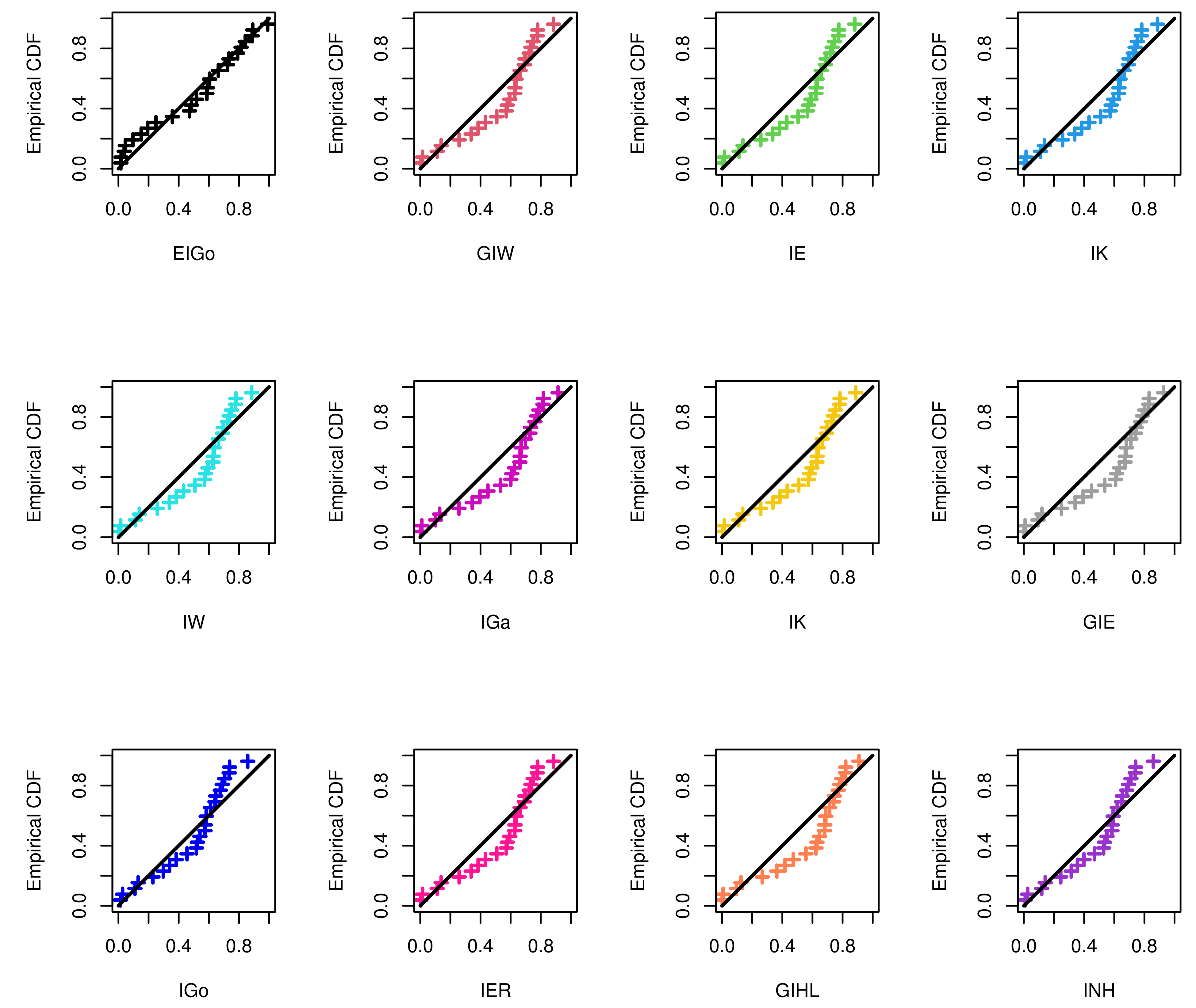
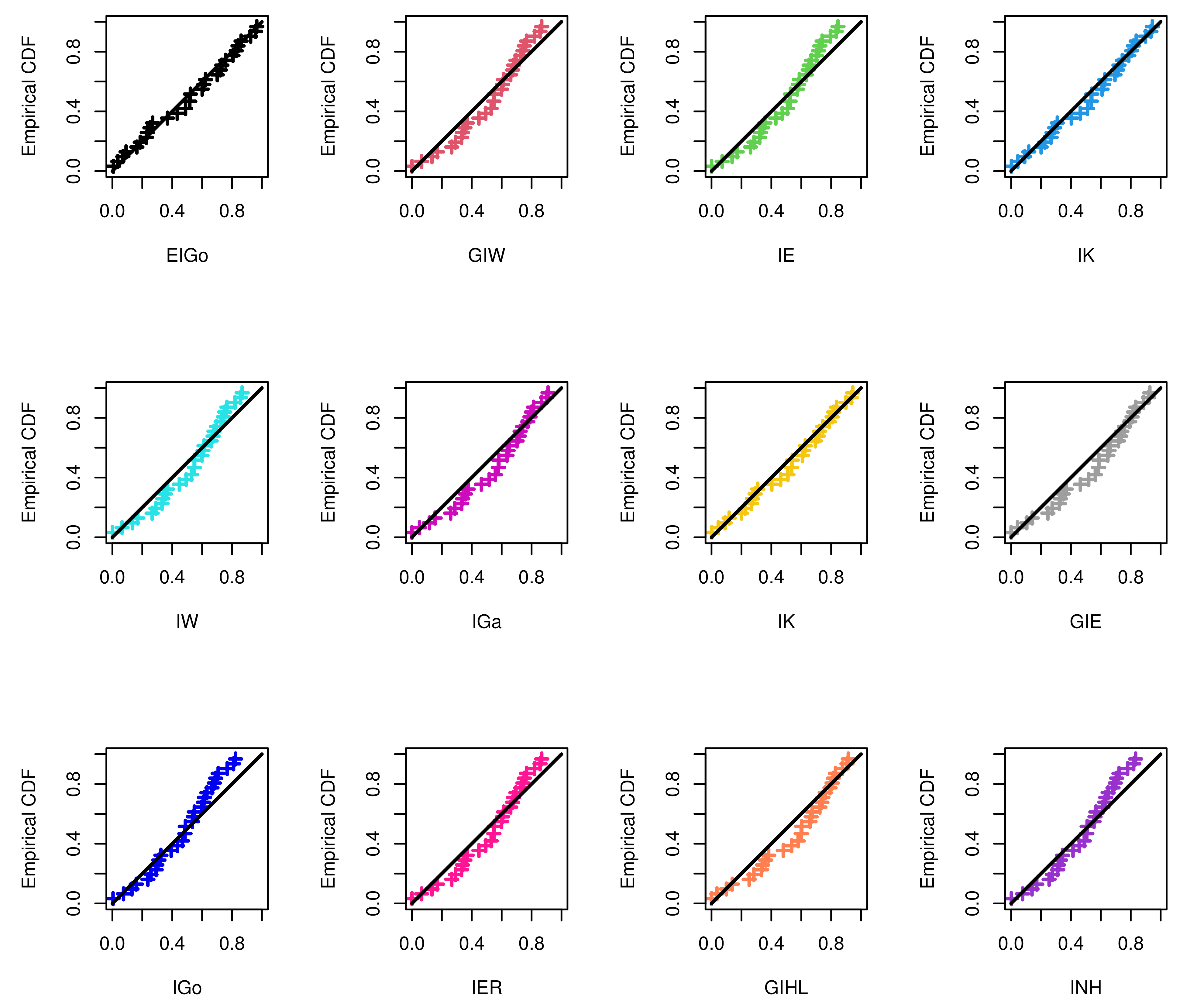
The R software and ML approach are adopted to estimate the parameters of the considered distributions and also to evaluate the goodness-of-fit measures. The calculated values of the ML estimates of the model parameters with their standard errors (SEs) and corresponding selection measures, for both data sets, are provided in Table 7 and Table 8, respectively. Moreover, Figure 3 and Figure 4 show graphically the quantile–quantile (Q–Q) plots of all competitive distributions for both datasets.
Table 7.
The estimates, SEs, and selection measures of the EIGo distribution and other competing models for first data.
Table 8.
The estimates, SEs, and selection measures of the EIGo distribution and other competing models for second data.
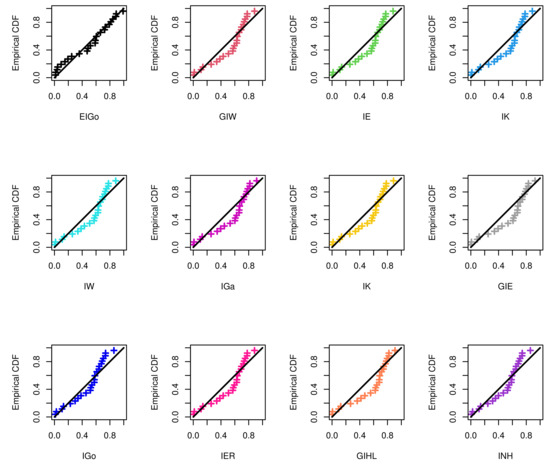
Figure 3.
The Q–Q plots of EIGo distribution and its competing models for first data.
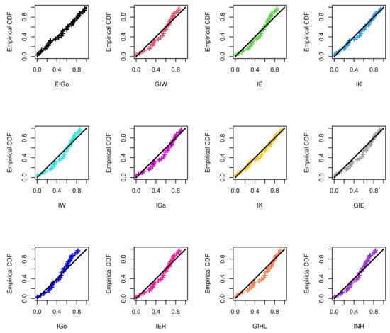
Figure 4.
The Q–Q plots of EIGo distribution and its competing models for second data.
Among all fitted competitive models, Table 7 and Table 8 show that the EIGo distribution has the lowest values of NCL, AIC, CAIC, BIC, HQIC, K-S, A-D, and CvM and the highest p-value. Consequently, the EIGo distribution provides better fit, for the given datasets, than the IGo and other inverted distributions. Furthermore, the relative histograms of both datasets and the fitted densities, as well as the plot of fitted and empirical survival functions (SFs), are displayed in Figure 5 and Figure 6, respectively. It is seen that, the graphical presentations in Figure 3, Figure 4, Figure 5 and Figure 6 support the numerical findings.

Figure 5.
The relative histogram and fitted densities of competing models (left) and fitted and empirical SFs (right) for first data.
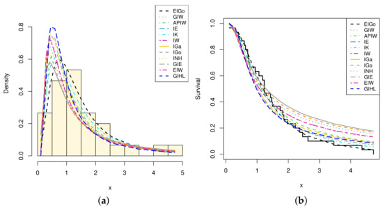
Figure 6.
The relative histogram and fitted densities of competing models (a) and fitted and empirical SFs (b) for second data.
7. Conclusions
In this paper, we have proposed a new three-parameter model called the extended inverse-Gompertz (EIGo) distribution. The EIGo model generalizes some well-known models such as the inverted-exponential, generalized inverted-exponential, and inverse-Gompertz distributions. Various statistical and reliability properties of the EIGo distribution have been addressed. The EIGo parameters have been estimated by the maximum-likelihood and Bayesian approaches under Type-II censoring. The performances of the maximum likelihood and Bayesian estimators have been examined by detailed simulation results. Based on our study, we recommend the Bayesian MCMC estimation of the parameters of the EIGo distribution using the hybrid Gibbs within M-H algorithm sampler. Finally, two real-life engineering data sets have been analyzed to illustrate the applicability of the EIGo distribution as compared with other competing models. The EIGo model provides an adequate and improved fit with respect to its competing inverted models. The failure rate of the EIGo model can only be upside-down-bathtub-shaped. Hence, for future works, the authors suggest that other extensions of the inverse-Gompertz distribution be proposed that may provide all important shapes for the hazard rate including increasing, bathtub, decreasing, and unimodal shapes.
Author Contributions
Conceptualization, A.E. and A.Z.A.; Funding acquisition, H.M.A.; Investigation, A.E.; Methodology, A.E., H.M.A. and A.Z.A.; Project administration, A.Z.A.; Resources, H.M.A.; Software, A.E.; Writing—original draft, A.E.; Writing—review and editing, H.M.A. and A.Z.A. All authors have read and agreed to the published version of the manuscript.
Funding
This study was funded by Taif University Researchers Supporting Project number (TURSP-2020/279), Taif University, Taif, Saudi Arabia.
Data Availability Statement
Not applicable.
Acknowledgments
The authors would like to thank the Editorial Board and the anonymous reviewers for their constructive comments and suggestions that improved the final version of the article.
Conflicts of Interest
The authors declare no conflict of interest.
References
- Gompertz, B. On the nature of the function expressive of the law of human mortality, and on a new mode of determining the value of life contingencies. In A letter to Francis Baily, Esq. FRS & C. Philos. Trans. R. Soc. Lond. 1825, 115, 513–583. [Google Scholar]
- El-Gohary, A.; Alshamrani, A.; Al-Otaibi, A.N. The generalized Gompertz distribution. Appl. Math. Model. 2013, 37, 13–24. [Google Scholar] [CrossRef] [Green Version]
- Jafari, A.A.; Tahmasebi, S.; Alizadeh, M. The beta-Gompertz distribution. Rev. Colomb. Estadística 2014, 37, 141–158. [Google Scholar] [CrossRef] [Green Version]
- Khan, M.S.; Robert, K.; Irene, L.H. Transmuted Gompertz distribution: Properties and estimation. Pak. J. Stat. 2016, 32, 161–182. [Google Scholar]
- Roozegar, R.; Tahmasebi, S.; Jafari, A.A. The McDonald Gompertz distribution: Properties and applications. Commun. Stat.-Simul. Comput. 2017, 46, 3341–3355. [Google Scholar] [CrossRef] [Green Version]
- El-Bassiouny, A.H.; El-Damcese, M.; Mustafa, A.; Eliwa, M.S. Exponentiated generalized Weibull-Gompertz distribution with application in survival analysis. J. Stat. Appl. Probab 2017, 6, 7–16. [Google Scholar] [CrossRef]
- Mazucheli, J.; Menezes, A.F.; Dey, S. Unit-Gompertz distribution with applications. Statistica 2019, 79, 25–43. [Google Scholar]
- Ieren, T.G.; Kromtit, F.M.; Agbor, B.U.; Eraikhuemen, I.B.; Koleoso, P.O. A power Gompertz distribution: Model, properties and application to bladder cancer data. Asian Res. J. Math. 2019, 15, 1–14. [Google Scholar] [CrossRef]
- Hoseinzadeh, A.; Maleki, M.; Khodadadi, Z.; Contreras-Reyes, J.E. The skew-reflected-Gompertz distribution for analyzing symmetric and asymmetric data. J. Comput. Appl. Math. 2019, 349, 132–141. [Google Scholar] [CrossRef]
- Nzei, L.C.; Eghwerido, J.T.; Ekhosuehi, N. Topp-Leone Gompertz Distribution: Properties and Applications. J. Data Sci. 2020, 18, 782–794. [Google Scholar] [CrossRef]
- Eghwerido, J.T.; Nzei, L.C.; Agu, F.I. The alpha power Gompertz distribution: Characterization, properties, and applications. Sankhya A 2021, 83, 449–475. [Google Scholar] [CrossRef]
- Wu, J.W.; Hung, W.L.; Tsai, C.H. Estimation of parameters of the Gompertz distribution using the least squares method. Appl. Math. Comput. 2004, 158, 133–147. [Google Scholar] [CrossRef]
- Soliman, A.A.; Abd-Ellah, A.H.; Abou-Elheggag, N.A.; Abd-Elmougod, G.A. Estimation of the parameters of life for Gompertz distribution using progressive first-failure censored data. Comput. Stat. Data Anal. 2012, 56, 2471–2485. [Google Scholar] [CrossRef]
- Dey, S.; Moala, F.A.; Kumar, D. Statistical properties and different methods of estimation of Gompertz distribution with application. J. Stat. Manag. Syst. 2018, 21, 839–876. [Google Scholar] [CrossRef]
- Louzada, F.; Ramos, P.L.; Nascimento, D. The inverse Nakagami-m distribution: A novel approach in reliability. IEEE Trans. Reliab. 2018, 67, 1030–1042. [Google Scholar] [CrossRef]
- Ramos, P.L.; Louzada, F.; Shimizu, T.K.; Luiz, A.O. The inverse weighted Lindley distribution: Properties, estimation, and an application on a failure time data. Commun. Stat.-Theory Methods 2019, 48, 2372–2389. [Google Scholar] [CrossRef]
- Afify, A.Z.; Ahmed, S.; Nassar, M. A new inverse Weibull distribution: Properties, classical and Bayesian estimation with applications. Kuwait J. Sci. 2021, 48, 1–10. [Google Scholar] [CrossRef]
- Eliwa, M.S.; El-Morshedy, M.; Ibrahim, M. Inverse Gompertz distribution: Properties and different estimation methods with application to complete and censored data. Ann. Data Sci. 2019, 6, 321–339. [Google Scholar] [CrossRef]
- Nadarajah, S.; Kotz, S. The exponentiated type distributions. Acta Appl. Math. 2006, 92, 97–111. [Google Scholar] [CrossRef]
- Abouammoh, A.M.; Alshingiti, A.M. Reliability estimation of generalized inverted exponential distribution. J. Stat. Comput. Simul. 2009, 79, 1301–1315. [Google Scholar] [CrossRef]
- Keller, A.Z.; Kamath, A.R.R.; Perera, U.D. Reliability analysis of CNC machine tools. Reliab. Eng. 1982, 3, 449–473. [Google Scholar] [CrossRef]
- Jeong, J.H. Statistical Inference on Residual Life; Springer: New York, NY, USA, 2014. [Google Scholar]
- Kayid, M.; Izadkhah, S. Mean inactivity time function, associated orderings, and classes of life distributions. IEEE Trans. Reliab. 2014, 63, 593–602. [Google Scholar] [CrossRef]
- Johnson, R.A. Stress-Strength Models for Reliability. In Handbook of Statistics; Krishnaiah, P.R., Rao, C.R., Eds.; Elsevier: Amsterdam, The Netherlands, 1988; Volume 7, pp. 27–54. [Google Scholar]
- Greenwood, J.A.; Landwehr, J.M.; Matalas, N.C.; Wallis, J.R. Probability weighted moments: Definition and relation to parameters of several distributions expressable in inverse form. Water Resour. Res. 1979, 15, 1049–1054. [Google Scholar] [CrossRef] [Green Version]
- Lazo, A.V.; Rathie, P. On the entropy of continuous probability distributions. IEEE Trans. Inf. Theory 1978, 24, 120–122. [Google Scholar] [CrossRef]
- David, H.A.; Nagaraja, H.N. Order Statistics; John Wiley & Sons: Hoboken, NJ, USA, 2004. [Google Scholar]
- Shaked, M.; Shanthikumar, J.G. Stochastic Orders and Their Applications; Academic Press: Boston, MA, USA, 1994. [Google Scholar]
- Lawless, J.F. Statistical Models and Methods For Lifetime Data, 2nd ed.; John Wiley & Sons: Hoboken, NJ, USA, 2003. [Google Scholar]
- Kundu, D. Bayesian inference and life testing plan for the Weibull distribution in presence of progressive censoring. Technometrics 2008, 50, 144–154. [Google Scholar] [CrossRef]
- Gelman, A.; Carlin, J.B.; Stern, H.S.; Dunson, D.B.; Vehtari, A.; Rubin, D.B. Bayesian Data Analysis, 2nd ed.; Chapman and Hall/CRC: Boca Raton, FL, USA, 2004. [Google Scholar]
- Lynch, S.M. Introduction to Applied Bayesian Statistics and Estimation for Social Scientists; Springer: New York, NY, USA, 2007. [Google Scholar]
- Tierney, L. Markov chains for exploring posterior distributions. Ann. Stat. 1994, 22, 1701–1728. [Google Scholar] [CrossRef]
- Roberts, G.O.; Gelman, A.; Gilks, W.R. Weak convergence and optimal scaling of random walk Metropolis algorithms. Ann. Appl. Probab. 1997, 7, 110–120. [Google Scholar]
- Elshahhat, A.; Elemary, B.R. Analysis for Xgamma parameters of life under Type-II adaptive progressively hybrid censoring with applications in engineering and chemistry. Symmetry 2021, 13, 2112. [Google Scholar] [CrossRef]
- Murthy, D.N.P.; Xie, M.; Jiang, R. Weibull Models; Wiley Series in Probability and Statistics; Wiley: Hoboken, NJ, USA, 2004. [Google Scholar]
- Keller, A.Z.; Goblin, M.T.; Farnworth, N.R. Reliability analysis of commercial vehicle engines. Reliab. Eng. 1985, 10, 15–25. [Google Scholar] [CrossRef]
- Glen, A.G. On the inverse gamma as a survival distribution. J. Qual. Technol. 2011, 43, 158–166. [Google Scholar] [CrossRef]
- Gusmão, F.R.; Ortega, E.M.; Cordeiro, G.M. The generalized inverse Weibull distribution. Stat. Pap. 2011, 52, 591–619. [Google Scholar] [CrossRef]
- Flaih, A.; Elsalloukh, H.; Mendi, E.; Milanova, M. The exponentiated inverted Weibull distribution. Appl. Math. Inf. Sci. 2012, 6, 167–171. [Google Scholar]
- Potdar, K.G.; Shirke, D.T. Inference for the parameters of generalized inverted family of distributions. ProbStat Forum 2013, 6, 18–28. [Google Scholar]
- Abd AL-Fattah, A.M.; El-Helbawy, A.A.; Al-Dayian, G.R. Inverted Kumaraswamy distribution: Properties and estimation. Pak. J. Stat. 2017, 33, 37–61. [Google Scholar]
- Tahir, M.H.; Cordeiro, G.M.; Ali, S.; Dey, S.; Manzoor, A. The inverted Nadarajah–Haghighi distribution: Estimation methods and applications. J. Stat. Comput. Simul. 2018, 88, 2775–2798. [Google Scholar] [CrossRef]
- Basheer, A.M. Alpha power inverse Weibull distribution with reliability application. J. Taibah Univ. Sci. 2019, 13, 423–432. [Google Scholar] [CrossRef] [Green Version]
Publisher’s Note: MDPI stays neutral with regard to jurisdictional claims in published maps and institutional affiliations. |
© 2021 by the authors. Licensee MDPI, Basel, Switzerland. This article is an open access article distributed under the terms and conditions of the Creative Commons Attribution (CC BY) license (https://creativecommons.org/licenses/by/4.0/).