The spontaneous emission of photons by an assembly of atoms in thermal equilibrium was considered by Einstein [
7] and by Dirac [
5] as fundamentally random. Einstein used statistics to describe an atom interacting with black-body radiation. In this case, there is a continuous process of excitation of the ground state by the black-body radiation, but practically, this is not a very efficient process compared to the excitation by a resonant monochromatic beam, which we shall consider. Thanks to the progress of experimental atomic physics, in 1986, Hans Dehmelt [
8,
9,
10] observed the leaping of electrons from one atomic state to another in individual atoms. This sudden transition of a tiny object (such as an electron, ion, molecule, or atom) from one of its discrete energy states to another has been called a quantum jump since Niels Bohr, who put this concept forward for discontinuous events, although Schrödinger (and others) strongly objected to their existence, postulating instead that they are not instantaneous.
Here, we study a simpler case, the emission of light by a two-level atom, an interesting worked example from the point of view of the statistical interpretation of quantum mechanics.
2.1. Towards a Full Statistical Theory of the Emission Process
We shall outline the principles of a statistical treatment that is able to describe both the emission of photons and the optical Rabi oscillations in the case of a single pumped two-level atom, detailed in [
11]; then, we shall explain how to derive the probability distribution of the time intervals between two successive photon-emission events. This was based upon the property that, in such an interval, the atom does make unhindered Rabi oscillations, and that the emission of a photon is a phenomenon seen as instantaneous. This is, of course, one basic feature of a Markov process because we consider quick jumps occurring at random with a probability depending on the state of the system and, possibly, on the absolute time. For such a phenomenon, the Kolmogorov equation seems to be the right tool to describe the state of an atom because this kind of equation describes the evolution of the probability distribution of a system under the effects of two processes, one leading to a deterministic dynamics, the other to random quasi-instantaneous events, as just written. Let
be the set of time-dependent parameters changing with time, with the time derivative
, a function of
. In the deterministic phase, the conservative and normalized probability
obeys the equation
where
is here and elsewhere for the derivative with respect to time, and
for the derivative with respect to
(This is actually a gradient in general because
has more than one component, but this only complicates the writing in an unessential way).
Kolmogorov equations add a right-hand side representing instantaneous transitions (or jumps) occurring at random instants of time to this equation, represented by a positive-valued function
. During a small interval of time
, if the system is in state
, it quickly jumps to state
with probability
so that the Kolmogorov equation describes both the deterministic dynamics and the jump process and reads [
12]:
In the right-hand side, the first positive term describes the increase in probability of the -state due to jumps from other states to . The second term represents the loss of probability because of jumps from to any other state . By integration over , one finds that the -norm is constant (if it converges, as we assume).
Let us now consider a two-level atom whose wave function is of the form
where
, the time derivative of
, is equal to
between two jumps,
being the Rabi frequency. The Kolmogorov equation deals explicitly with the probability distribution
for the atomic state, here indexed by a single variable
.
In the right-hand side of Equation (
2), the probability
for the atom to make a quantum jump from the state
towards the state
is proportional to
(where
is the Dirac distribution) because any jump lands on
in the interval
, and this probability is proportional to
because it comes from the state
with the squared amplitude
, and
is the emission rate of the atom in the excited state calculated by Dirac [
5]. Therefore,
Thus, the Kolmogorov equation for the two-level atom illuminated by a resonant pump field is
Introducing a probability distribution depending on a continuous variable, here, which amounts to putting a probability on the elements of the atomic density matrix, is a way to take into account all possible trajectories emanating from the emission of a single photon, with a new value of the number of photons radiated in any direction at each quantum jump. Average values of a time-dependent quantity that depends on can be calculated via the probability distribution , which is a -periodic function with a finite jump at , but smooth elsewhere. This procedure allows us to deal correctly with the infinite number of possible trajectories, since Boltzmann’s genius lies precisely in transforming the classical statistical theory based on unknown initial conditions into statistics for an ensemble of indeterminate trajectories.
We insist that our description of the fluorescence of a single two-level atom goes beyond solving Heisenberg equations (which is impossible anyway without making a strong hypothesis because of the infinite number of degrees of freedom of the EM field). Here, as in the quantum mechanical frame, the infinite number of degrees of freedom are taken care of because they represent the fast phenomena, which are well approximated in Dirac’s calculation of the coefficient
for the black-body radiation calculus. Moreover, the whole story before and after each rapid event is told here through the balance terms written in the right-hand side of the Kolmogorov equation, which has a built-in conservation law of the total probability at any time, a serious advantage with respect to the quantum treatments using a Lindblad equation [
13], which is difficult to handle [
14].
Because it is linear, Equation (
5) can be solved in a Laplace transform, but the general solution in time requires the inversion of a Laplace transform, which can be done only formally. There are two constraints: (i) The probability
is positive or zero and (ii) the total probability
is unity at any time, which reflects the unitary evolution of the atomic state (the integral of the square modulus of the wave function is constant and equal to one). It is relatively easy to check that they are fulfilled, since
is constant and
at any positive time if
. Solutions in various limits are derived in [
11]. The factors
on the right-hand side are there to take into account that a quantum jump occurs only if the atom is in the excited state, which has probability
. The negative term on the right-hand side is the loss term representing the decrease in the amplitude of the excited state by jumps to the ground state, whereas the positive one is for the increase in the amplitude of the ground state when a jump takes place.
The populations of the two levels, or probabilities for the atom to be in the excited or in the ground state at time
t, are, respectively,
and
Their sum is one, as it should be, if is normalized to one.
From (
5), one can derive an equation for the time derivative of
and
by multiplying (
5) by
and by
and integrating the result over
. This gives
and
On the r.h.s of the rate Equations (
8) and (
9), the first term, proportional to the Rabi frequency
, describes the effect of the Rabi oscillations, whereas the second term, proportional to
, displays the effect of the quantum jumps responsible for the photo-emission. Because
includes both the fluctuations due to the quantum jumps and the streaming term, the right-hand side of (
8) and (
9) represents the new history beginning at each step. After integration by parts, (
8) and (
9) become
Note that the set of Equations (
8) and (
9), or (
10), is not closed. It cannot be mapped into equations for
and
only because their right-hand sides depend on higher momenta of the probability distribution
, momenta that cannot be derived from the knowledge of
and
. The unclosed form of (
8) and (
9) is a rather common situation. To name a few cases, the BBGKY hierarchy of non-equilibrium statistical physics makes an infinite set of coupled equations for the distribution functions of systems of interacting (classical) particles [
15], where the evolution of the one-body distribution depends explicitly on the two-body distribution, which depends itself on the three-body distribution, etc. In the theory of fully developed turbulence, for instance, the average value of the velocity depends on the average value of the two-point correlation of the velocity fluctuations, depending itself on the three-point correlations, etc. Fortunately, one can solve the Kolmogorov Equation (
5) via an implicit integral equation [
11]; then, there is generally no need to manipulate an infinite hierarchy of equations as in those examples.
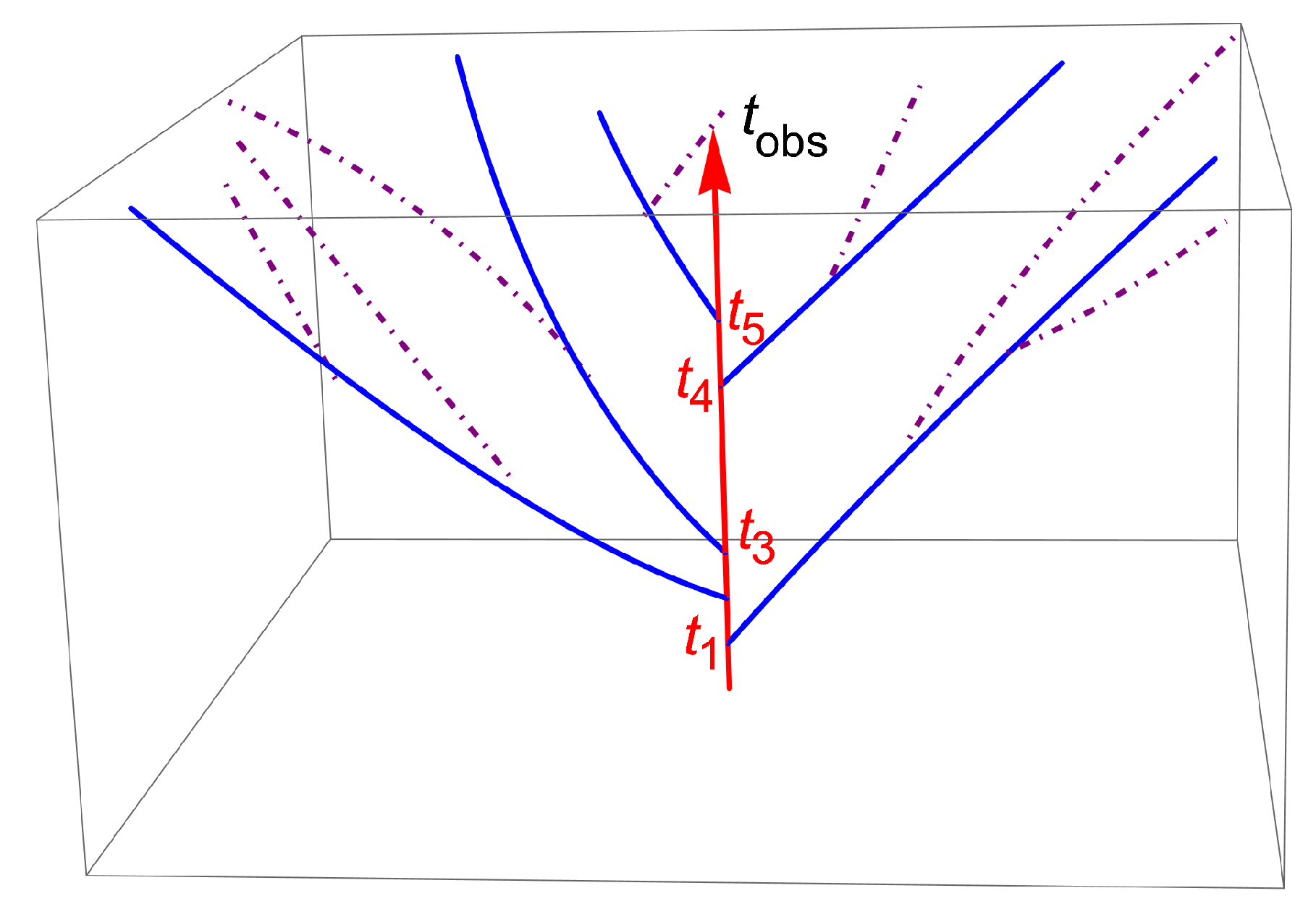
In the present case, one can say, following Everett, that the probability distribution
allows one to make averages over the states of the atom in different universes, each being labeled by a value of
at a given time
t. As written above, physical phenomena such as the observation of a quantum state decay measured by emission of a photon are relative to the measurement apparatus that takes place in the universe associated with the observer. At every emission of a photon, a new history begins, represented by the right-hand side of (
9). In summary, the creation of new universes at each step defines a Markov process, which can be described by a Kolmogorov statistical picture, and cannot be considered as a deterministic process depending in a simple way on averaged quantities, such as population values.
2.2. Quantum Jump Statistics
To illustrate how one can use the Kolmogorov equation, we derive the time-dependent probability of photo-emission by a single atom, first without any pump field, then in the presence of a resonant laser.
We consider first an isolated atom initially in pure state
given by (
3) with
. The solution of (
5) with
(no pump) and
is
The evolution of the probability that the atom is in the excited state at time
t is given by (
6), and the emission of a photon occurs randomly in time with a rate:
Once the atom “jumps” to its ground state, it cannot emit another photon; then, the emission of a photon, if recorded, is a way to measure the state of the atom. The solution of (
12) leads to the population of the excited state
when taking into account the initial condition, and the photo-emission rate is
The probability of photo-emission in the interval
is the integral of
:
which means that the final state of the coupled system of the atom plus the emitted photon field is
where the indices (1, 0) correspond to the one and zero photon states, respectively. The relation (
15) means that if we consider
N atoms initially prepared in a given pure state with
, namely, with total energy
, we get, at infinite time,
N atoms in the ground state and
photons of individual energy
. In the final state, only a fraction of them,
, jump from the excited state to the ground state with the emission of a photon; the others,
, simply stay in the ground state [
16].
In the case of an atom submitted to a resonant pump field, the atom will emit photons at random times, forming a point process. Here, we assume that the process is Markovian, but more generally, any process with time-dependent history is completely characterized by its conditional intensity function
, the density of points at time
t, where
is the history of the emission activity up to time
t, and the time interval probability distribution is given by the relation
. In the present Markovian case, the conditional intensity of the point process, which is the probability of emission of a photon at time
t, only depends on the value of
at this time; therefore, one simply has
. From (
8), we deduce
In this relation, the exponent 4 comes from two conditions: One in which the atom is in the excited state, and the other in which it emits a photon, as in (
14), which describes an emission without any pump field. With a pump field, in between two successive emission times, the atom undergoes Rabi oscillations with
, assuming that a photon is emitted at time
. Therefore, the inter-emission time distribution for an atom driven by a resonant pump is given by the expression [
17]:
which gives
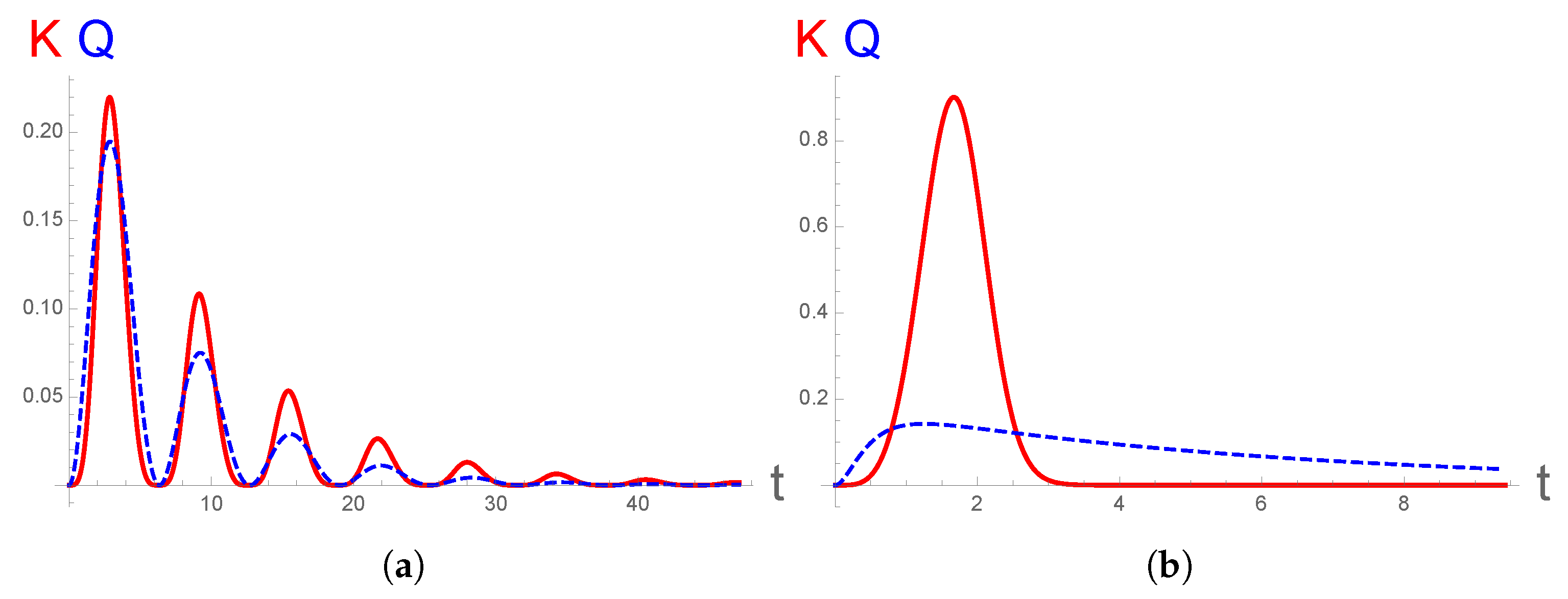
, as expected. The result is shown in
Figure 1 in the two opposite limits of large and small values of the ratio
and is compared to the delay function derived in [
18,
19] (which does not have the standard form expected for a Markovian process). For the case of a strong input field,
, the two methods approximately agree; see
Figure 1a. However, they differ noticeably in the opposite case, which is shown in
Figure 1b. For weak laser intensity (or strong damping), the Kolmogorov derivation gives a mean delay between successive photons of order
, which decreases slowly as the damping rate
increases, which seems reasonable. In the same limit, the dressed atom method leads to
, a time scale much longer than the inverse of
, and increasing with the damping rate, a result that seems to go against intuition [
20].
2.3. Relationship with Planck-Einstein Theory
The above analysis of the spontaneous emission was devoted to an atom (or an ensemble of independent atoms) initially prepared in the pure state
In this case, the non-diagonal component of the atomic density matrix evolves as
This case—the so-called “coherent case”—displays a rate of emission of photons that is not equal to
, the line-width of the excited state, but is equal to
. Then,
depends in a non-trivial way on the atomic state. This points to a potentially interesting feature because the rate decreases when
decreases; therefore, the atom is maintained in the excited state longer than in the case of black-body radiation, where the decay rate is
, as was deduced by Planck and Einstein. In the latter case, the atoms are in thermal equilibrium (an incoherent state with
), with a probability
of being in the ground state or
p of being in the excited state. At equilibrium, the probability
is
Taking expression (
21) as an initial condition, the problem reduces to the one treated in
Section 2.2 with
and
. The solution of the Kolmogorov equation is then given by (
11), and the non-diagonal component of the atomic density matrix is given by (
20). The important point is that the decay rate is equal to the constant
without the factor
(when taking
in these equations), and the non-diagonal components of the density matrix vanish at any time, as expected for an incoherent state.
This permits to understand where the factor in the decay constant comes from. Let us associate this result with the Dirac expression for . In Dirac’s calculation, is proportional to the square modulus of the excited-state amplitude of the wave function because he considered a problem of evolution in general. From the point of view of Everett’s multiple worlds, this amplitude depends on the universe in which the atom evolves. If , one knows that the atom may belong to the set of atoms that are in the excited state with a probability of one, and no reduction factor has to be associated with the decay rate . However, if , one cannot assume that the atom is in the excited state with a probability of one. Therefore, there is, a priori, a reduction factor (less than 1) to be included in Dirac’s formula for the rate .


