Abstract
It has recently been shown in the Eastern Mediterranean that by combining natural time analysis of seismicity with earthquake networks based on similar activity patterns and earthquake nowcasting, an estimate of the epicenter location of a future strong earthquake can be obtained. This is based on the construction of average earthquake potential score maps. Here, we propose a method of obtaining such estimates for a highly seismically active area that includes Southern California, Mexico and part of Central America, i.e., the area NW. The study includes 28 strong earthquakes of magnitude M that occurred during the time period from 1989 to 2020. The results indicate that there is a strong correlation between the epicenter of a future strong earthquake and the average earthquake potential score maps. Moreover, the method is also applied to the very recent 7 September 2021 Guerrero, Mexico, M7 earthquake as well as to the 22 September 2021 Jiquilillo, Nicaragua, M6.5 earthquake with successful results. We also show that in 28 out of the 29 strong M EQs studied, their epicenters lie close to an estimated zone covering only 8.5% of the total area.
1. Introduction
Earthquakes (EQs) in Mexico and the surrounding region of Southern California and Central America are very common and extremely strong, see, e.g., References [1,2,3,4] and references therein. When focusing in the region NW (shown in Figure 1), more than twenty-eight EQs with a magnitude M have occurred there since 1989. In the present paper, we employ the natural time analysis (NTA) [5,6,7,8,9,10] and earthquake nowcasting (EN) [11,12,13,14,15,16,17,18] aiming at forecasting the epicenter of such a strong future EQ.
Recently, our group has combined [19] NTA and EN together with the properties of the earthquake networks based on similar activity patterns (ENBOSAP) [20,21] for a similar purpose in the Eastern Mediterranean region where seismicity is much less intense than in the region NW of our present interest. We see that when strong EQs are frequent, as is the present case, we can simplify the approach of Reference [19] just by using NTA and EN.
Natural time was introduced [5] in 2001 as a general method to analyze time-series resulting from complex systems [7]. It has been applied to a variety of fields, such as condensed matter physics [22,23,24], geophysics [6,25,26,27,28,29,30,31,32,33,34], civil engineering [35,36,37,38], climatology [39,40,41,42], and biomedical engineering [43,44]. Within the concept of NTA, it has been shown that the variance of natural time may be considered as an order parameter for seismicity [3,45,46,47,48,49] as well as in acoustic emission before fracture [28,50] or in other self-organized critical phenomena such as ricepiles [51] and avalanches in the Olami–Feder–Christensen [52] earthquake model [53] or in the Burridge–Knopoff [54] train model [55]. Especially for seismicity, the study of this order parameter by means of its variability [56] revealed [9,21,57,58,59,60,61,62,63] the presence of characteristic minima before the occurrence of strong EQs. Interestingly, the precursory Seismic Electric Signals (SES) activities [64,65], which are a series of low frequency electric signals ( 1 Hz) observed before strong EQs [64,65,66,67,68,69,70] have been shown to appear [19,71,72] almost simultaneously with the variability minima.
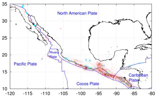
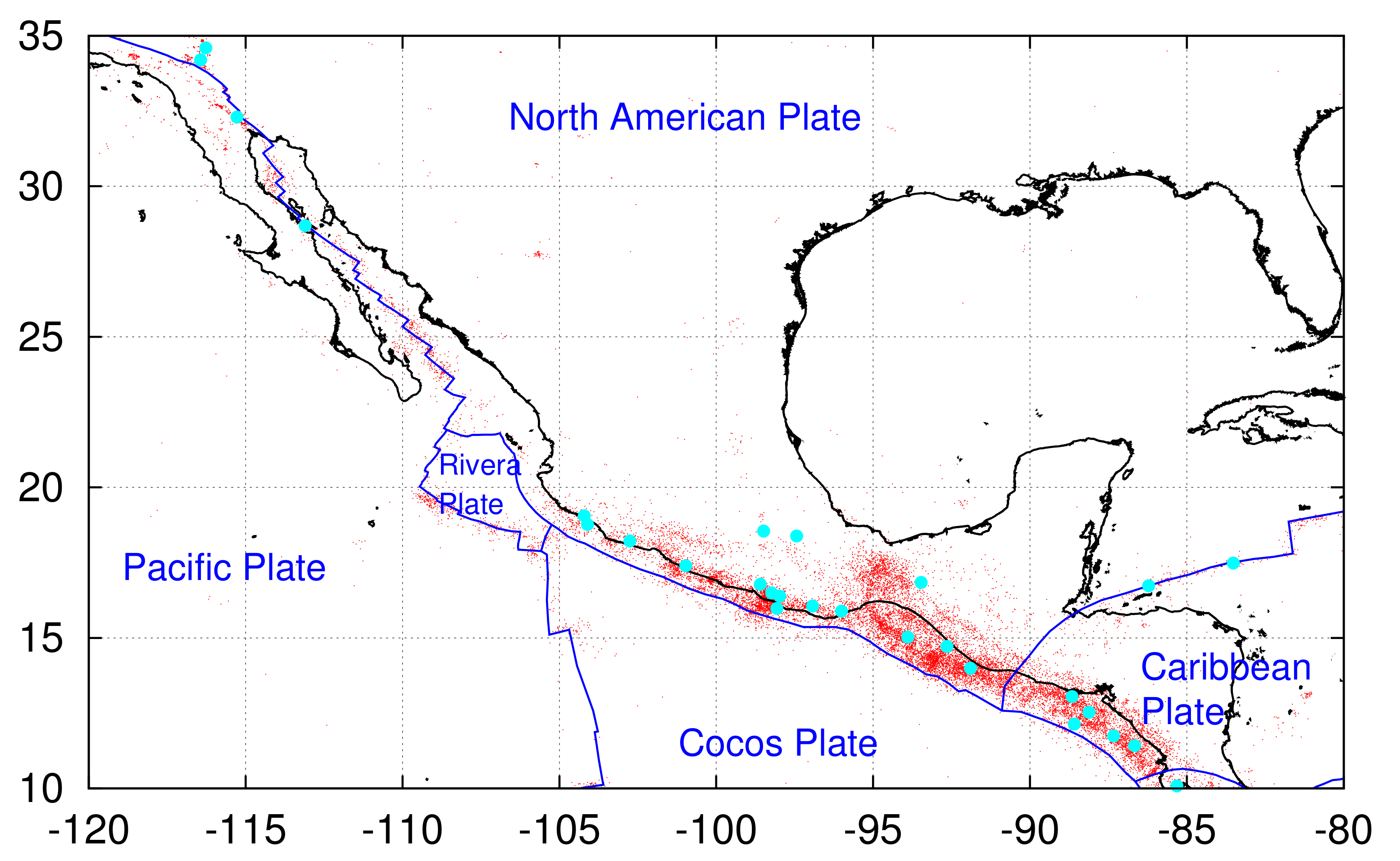
Figure 1.
Map of the study area NW together with the plate boundaries (blue) according to Bird [73]. The epicenters of the 28 strong EQs with during 1989 to 2020 are shown with cyan bullets while those of the EQs with by red dots.
Figure 1.
Map of the study area NW together with the plate boundaries (blue) according to Bird [73]. The epicenters of the 28 strong EQs with during 1989 to 2020 are shown with cyan bullets while those of the EQs with by red dots.
Earthquake nowcasting has been introduced by Rundle et al. [11] and allows the evaluation of the current state of seismic hazard for strong EQs by the number of smaller EQs that occur in the time interval between two strong ones. It has been applied for the estimation of seismic risk to global megacities [12,15] as well as of the risk of great earthquakes that may generate mega-tsunamis [74]. EN has also been applied for the estimation of induced seismicity [75,76] and offers unique possibilities for the estimation of the seismic risk worldwide through global sources of seismic catalogs, see, e.g., References [77,78,79,80], cf. local EQ catalogs have also been used, such as the one from the Institute of Geodynamics of the National Observatory of Athens [81,82,83] for EN in Greece (Chouliaras, personal comm. 2019).
2. Materials and Methods
2.1. EQ Data and the Tectonics of the Study Area
The area of interest here is Southern California, Mexico, and Central America, see Figure 1. We used the United States National Earthquake Information Center (NEIC) PDE catalog—these data are available from the United States Geological Survey (USGS), cf. [84]—in the region NW and considered all EQs recorded during the period of almost 50 years from 1 January 1973 to 21 September 2021 with magnitude .
The interaction of the continental block with the oceanic provinces that surround Mexico has resulted in the current geographic layout. Mexico is located in a region where five tectonic plates: North America, Pacific, Rivera, Cocos, and Caribbean, are in regular interaction. The major fault zones, the spreading zones, and the subduction zones determine the boundaries between these plates [85]. The North America’s displacement is to the southwest, the Eastern Pacific’s to the northwest, the Cocos and Rivera’s to the northeast, and the Caribbean’s to the east; this disposition enhances the likelihood of a large seismic occurrence. Mostly, the interplay that occurs on the Mexican Pacific’s southern coast, where the Cocos plate subducts beneath the North American plate, is the primary source of earthquakes in this country.
Oceanic plates are considered to be substantially more rigid than continental plates due to their olivine-rich composition. The Pacific Plate, the largest of the Earth’s tectonic plates, is extensively an oceanic plate. The plate border deformation zones in the continental crust are, without a doubt, far larger (tens to hundreds of kilometers) than the normally narrow (10 km) boundaries seen in oceanic plates [86]. In the Pacific region, the Baja California Peninsula is moving northwest, separating from the rest of the continent; the oceanic plate of the Cocos is being assimilated by the continent in the southern Pacific of Mexico, from Cabo Corrientes in the state of Jalisco to Central America; this subduction occurs along an oceanic trench known as the Acapulco or Mesoamerican megashear [87]. Further, in the seismic regions of the Gulf of Mexico and the Caribbean there are geological forces of cortical separation (also referred as tension or distensive) operating on the continental limits, and as a result of the movement of the continental tectonic plates of North America towards the west and the Caribbean towards the east, they advance on the deepest bottoms of the oceanic basins. In the Pacific Plate, in southern California and in Baja California, the plates are migrating northwesterly relative to the North American plate along a series of transformation faults (San Andreas fault) connecting the extension centers, whose activity is gradually separating this territory from the rest of the continent, for which it will become an island in approximately 10 million years. Similarly, oceanic faults allow magma to escape, generating an expansion of the ocean floor [88,89].
The Rivera microplate is located in southern Baja California, right at the gateway to the Sea of Cortez where the magnetic lineaments of the ocean floor indicate how the gap between the Pacific plate and the Rivera plate, positioned between fracture zones, grows. Due to the movement that the Cocos and Rivera plates have towards the northeast of the Mexican Republic, a portion of these plates dips under the North American plate, causing great earthquakes to occur along the coast of Jalisco, Colima, Michoacán, Guerrero, Oaxaca, and Chiapas; yet we cannot determine if these large earthquakes were caused by the Cocos or Rivera plate movement. The Cocos plate is built in the Eastern Pacific mountain range, that goes from the Rivera fault zone to the Galapagos mountain chain. It is located off the coastlines of Michoacán, Guerrero, Oaxaca, and Chiapas, and it dips into the continental crust, leading to a displacement that causes earthquakes throughout the Pacific coast.
Cocos plate subducts beneath the North American plate at a rate of about 12 cm/yr from 20 Ma to 11 Ma and 6 cm/yr from 11 Ma to present [90]. Along the central portion of the Middle American Trench, the subduction interface shows a significant variety in along strike dip angles; also, the middle section of the plate, near Acapulco, has a horizontal slab. The trace/strike of the Neogene volcanic arc, which trends at a 17 degree angle to the trace/strike of the trench, demonstrates the along strike change in the dip. The dip is 50 degrees to the northwest near the Rivera Plate junction, and 30 degrees to the southeast near the Tehuantepec Ridge [91]. The slab in central Mexico has returned to its current location near the southern boundary of the Neogene volcanic arc, as shown by the southward movement of the volcanic arc [92].
A triple point to the southeast of the Tehuantepec Ridge divides the North American plate from the Caribbean plate, and the Cocos plate begins to subduct under it; this poses substantial natural hazards to most of central and southern Mexico. The Yucatan Peninsula, for its part, is rotating clockwise, and the Trans-Mexican Volcanic Belt is still active [93].
2.2. Natural Time Analysis Background: An Order Parameter for Seismicity and Its Minima
The natural time for the occurrence of the k-th EQ of the energy in a time series comprising N EQs is defined as . Hence, the evolution of the pair is studied in the NTA, where
is the normalized energy and is estimated by means of the relation [94] , where stands for the EQ magnitude. The variance of natural time weighted for , namely
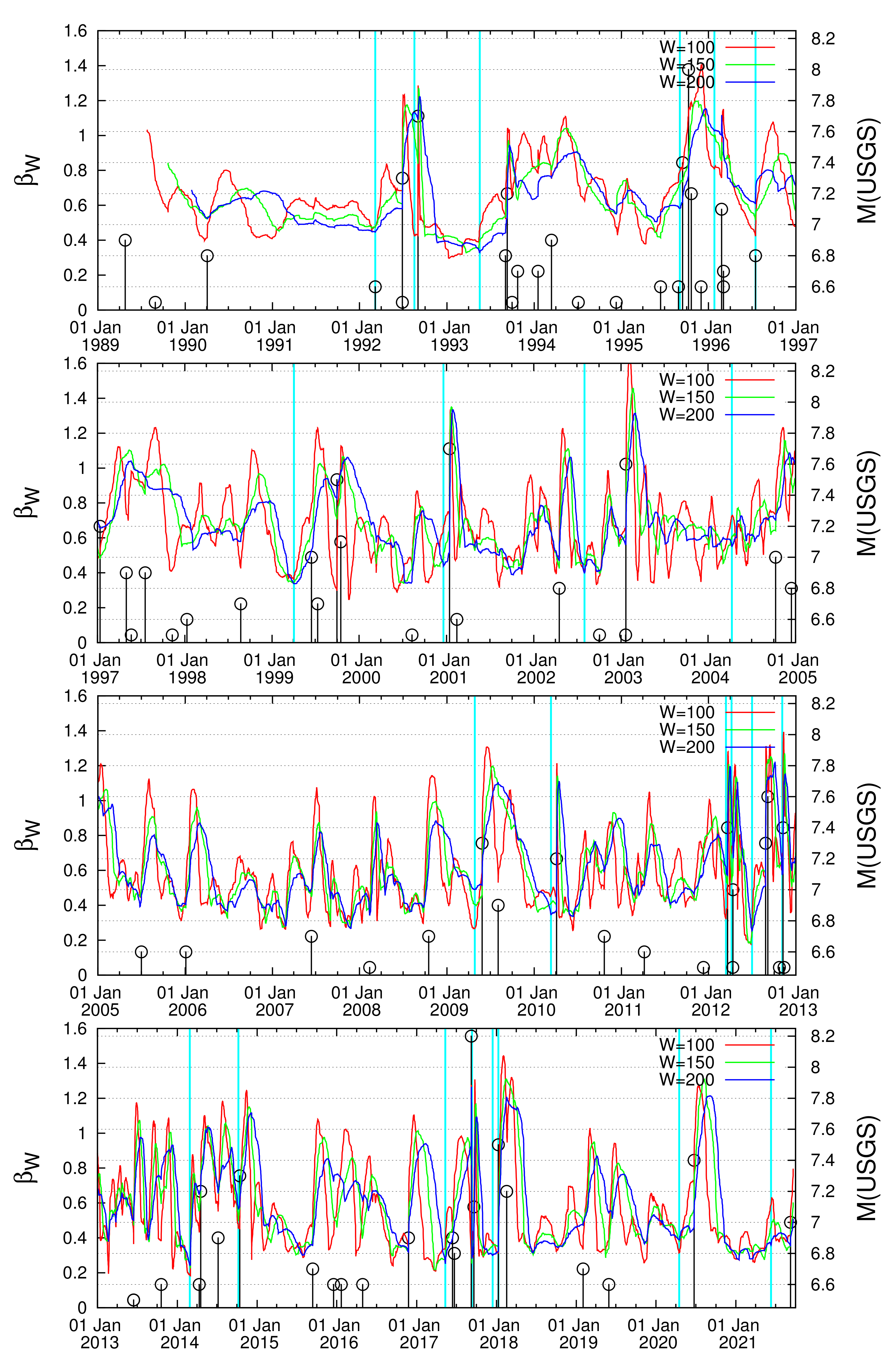
can be considered as an order parameter for seismicity [45]. The fluctuations of this order parameter of seismicity in an EQ catalog can be studied by using a fixed-length sliding natural time window containing a number W of consecutive EQs by means of the procedure described in References [9,95]. The window length W is selected to correspond to the average number of EQs that occur within the crucial scale [96] of a few months, or so, which is the average lead time of SES activities. To this end, we estimate all the values from the subexcerpts of consecutive 6 to W EQs within the excerpt of the EQ catalog of W EQs and use them for the calculation of their average value and standard deviation . The variability of the order parameter of seismicity is given by [7,56]
while its temporal evolution can then be pursued by sliding the natural time window of W consecutive EQs, event by event through the EQ catalog, see Figure 2 and Figure 3. In such a procedure, we assign to the occurrence time of the EQ which follows the last event of the excerpt of W EQs in the catalog.

Figure 2.
The variabilities for W = 100, 150, and 200 consecutive EQs versus the conventional time for the period 1989 to 21 September 2021. The EQ magnitudes (right scale) are depicted by the (black) vertical lines ending in circles. The cyan vertical lines indicate the dates at which minima of have been observed and have been selected for drawing the ⟨EPS⟩ maps.
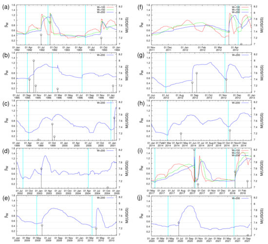
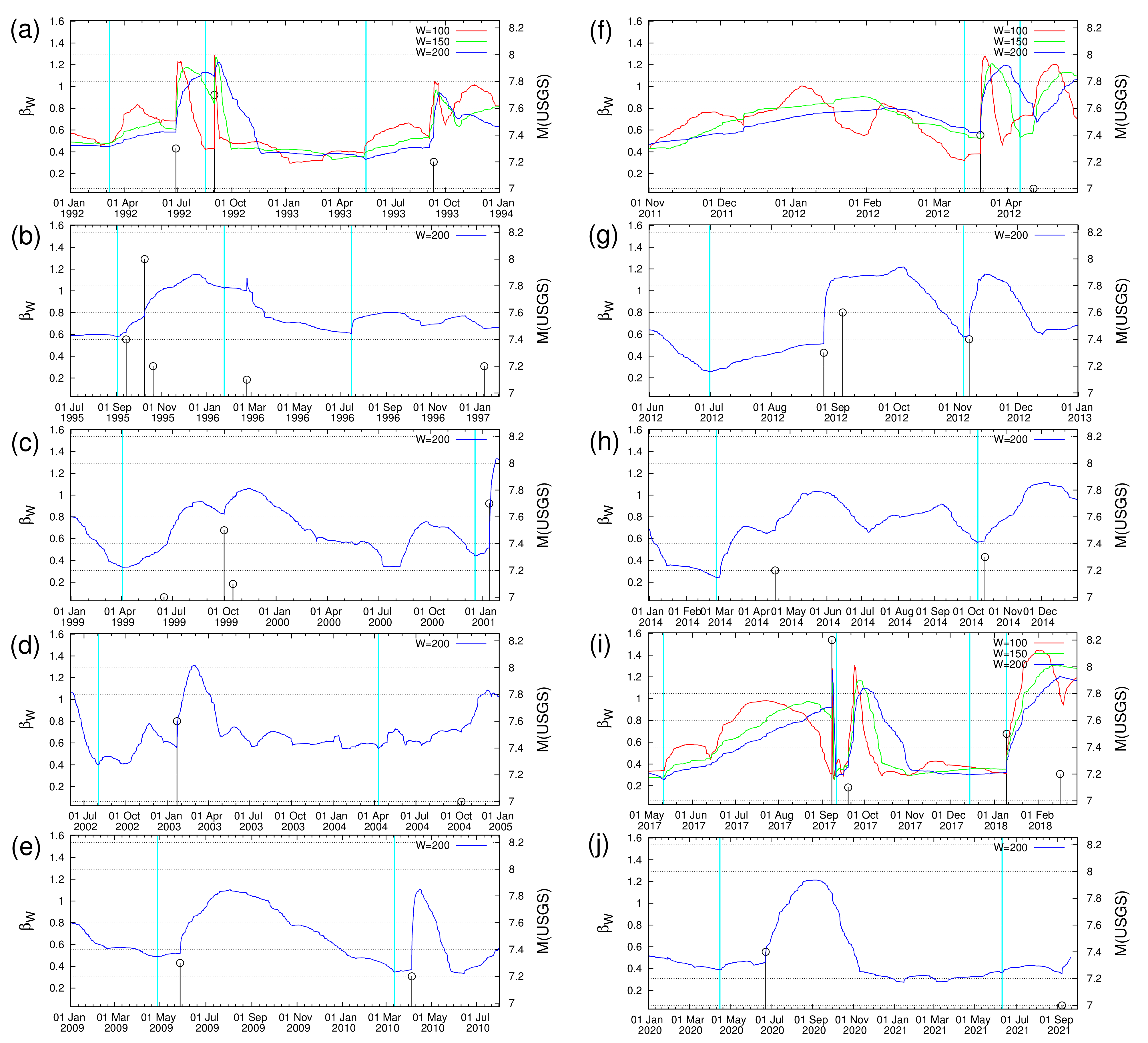
Figure 3.
Excerpts of Figure 2 in expanded time scale. Each excerpt (a)-(j) corresponds to a different time period, in which strong M EQs occurred: (a) 1992-1993, (b) 1995-1997, (c) 1999-2001, (d) 2003-2004, (e) 2009-2010, (f) March and April 2012, (g) August, September, and November 2012, (h) 2014, (i) 2017-2018, and (j) 2020-2021. In each panel, the variability is drawn while and are drawn only in the cases in which a minimum is identified based on 150 or 100 (see the text and Table 1).
2.3. Earthquake Nowcasting and Earthquake Potential Score
Rundle et al. [11] proposed EQ nowcasting as a method for estimating the seismic risk through the current state of fault systems in the progress of the EQ cycle identified on the basis of natural time (cf. more recently the construction of time series resembling the EQ cycle has been extensively studied in References [16,18,97]). To estimate the seismic risk, EN uses an EQ catalog to calculate from the number of ‘small’ EQs, defined as those with magnitude but above a threshold , i.e., , the level of hazard for ‘large’ EQs. As mentioned in the Introduction, the EQ catalogs adopted [11,12,19,77,78,79,80,98] are global seismic catalogs such as the Advanced National Seismic System Composite Catalog or the NEIC PDE catalog and for the completeness threshold of the EQ catalog is usually selected [11]. Along these lines, the magnitude threshold has been considered [12,78] for applications in areas such as Greece, Japan, and India that lie outside the United States. In EN, one employs the natural time concept and counts the number n of ‘small’ EQs that occur after a ‘large’ EQ—n stands for the waiting natural time or interoccurrence natural time. Then, the current number of the ‘small’ EQs since the last occurrence of a ‘large’ one is compared to the cumulative distribution function (CDF) of the interoccurrence natural time . To estimate , it should be ensured [11] that we have enough data to span at least 20 or more ‘large’ EQ cycles. In EN, the EQ potential score (EPS) equals the CDF value,
and measures the level of the current hazard, see Figure 4a. In References [11,12,77,78,79] the seismic risk for various cities of the world was estimated through the following procedure: After calculating the CDF within a large area, the number of the small EQs around a city, i.e., those occurring within a circular region of epicentral distances since the occurrence of the last ‘large’ EQ in this circular region, is found. Given that EQs exhibit ergodicity—see, e.g., References [99,100,101]—Rundle et al. [12] suggested that the seismic risk around a city can be estimated by using the EPS corresponding to the current value of by inserting in Equation (4).
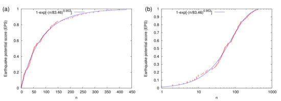
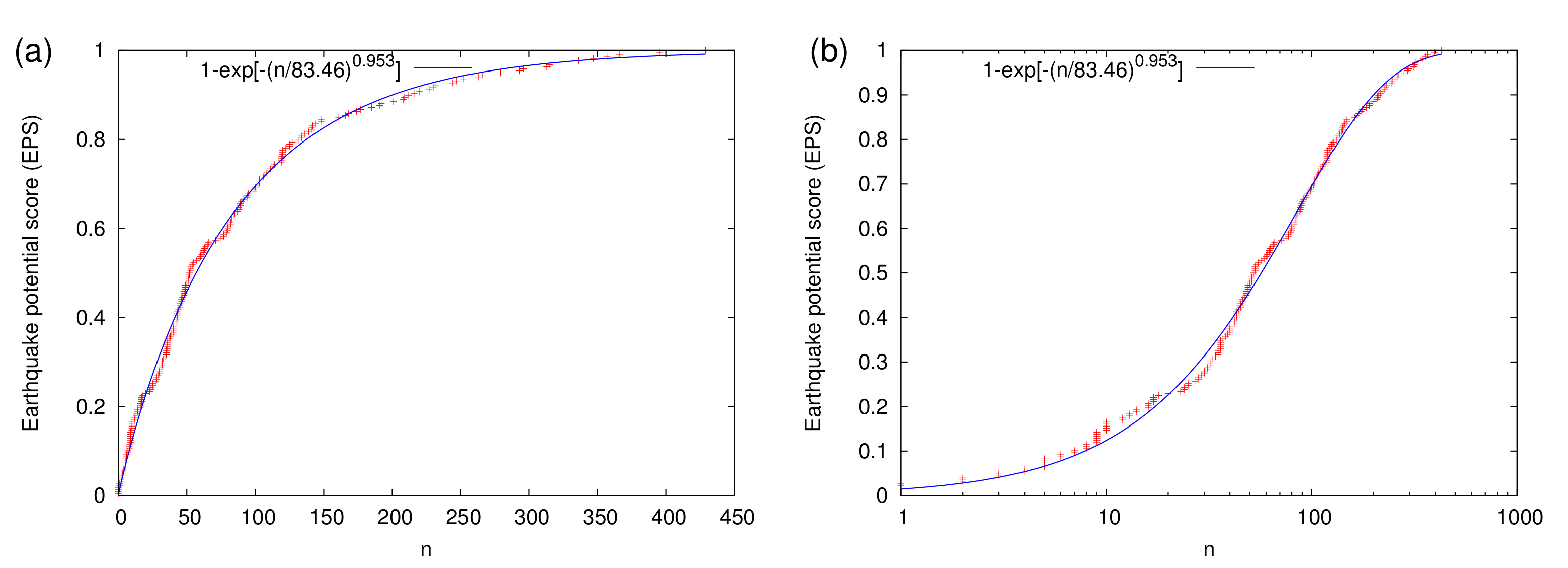
Figure 4.
The empirical cumulative distribution function (red plus symbols) of the number n of EQs with M that occur between two EQs of magnitude M in the study area NW of Figure 1 during the period 1989 to 2020. This equals to the EPS according to EQ nowcasting and has been calculated on the basis of 218 EQ cycles. The corresponding Weibull model fit [79] is also shown with the blue curve in lin–lin (a) and lin–log (b) diagram.
In the present study, the area considered is NW, which for and leads to the CDF shown in Figure 4a. When focusing on the period from 1 January 1989 to 1 January 2021, the empirical CDF comprises 218 EQ cycles and is shown in Figure 4a. In this figure, we observe that the fit
using the Weibull distribution provides a fair approximation with root mean square of residuals [102] equal to 0.0177. This property of the Weibull distribution is in accordance with the results found by Pasari and Sharma [79] for Himalayan EQs as well as with those later found in Reference [19] for Eastern Mediterranean.
2.4. Construction of Average Earthquake Potential Score Maps
Upon the selection of a date, one can estimate by means of the EQ catalog the number of ‘small’ EQs that occurred since the last ’large’ EQ inside a circle of radius R for each point in the study area. By inserting in Equation (5) we can obtain the corresponding EPS value. The ⟨EPS⟩ maps are constructed by evaluating first the value of EPS, EPS, at the points of a ‘square’ lattice that covers the study area and then by spatially averaging these EPS values within disks of the same radius R:
where the summation is restricted to the lattice points whose distance from the observation point is smaller than or equal to R; N stands for the number of lattice points included in the sum.
In Section 3 of Reference [19], it has been shown that the ⟨EPS⟩ mean value
where the summation is made over all the lattice points , estimated numerically in an ⟨EPS⟩ map drawn with self-consistency radius R and covering an area A of average radius may take the form
where is related to [19] the fractal dimension [103] of EQ epicenters.
3. Results
A self-consistent method of producing ⟨EPS⟩ maps using a radius R has been suggested and applied to Eastern Mediterranean in Reference [19], as already mentioned. The date on which has been observed -on the basis of the analysis of the properties of ENBOSAP [21]- has been selected for drawing these ⟨EPS⟩ maps. The latter are produced by first estimating EPS for disks of radius R centered at each point of a square 0.25 lattice covering the whole region of study and then by averaging these EPS values within the same radius R (see Section 2.4). A clear relation between the such made ⟨EPS⟩ maps and the epicenter of an impending strong EQ has been observed. Moreover, the stability of the method when changing the lattice ‘constant’ from 0.25 to 0.10 has been secured.
Here, we focus on the area NW of intense seismicity depicted in Figure 1. For example, during the 32 year period from 1 January 1989 to 1 January 2021 we have in total 19,184 EQs with M , i.e., approximately 50EQs/month, 28 of which have magnitude M , i.e., approximately 0.875 EQs/year (see Table 1). Due to this frequent occurrence of EQs of magnitude M , the application of the properties of ENBOSAP k-cores in order to identify the minima preceding these strong EQs as made in Reference [19] is not considered necessary. In other words, since on average every year we have approximately one strong EQ we just need to identify minima of the variability for a reasonable value of W as suggested by Varotsos et al. [96]. We selected corresponding to the number of EQs that occur on average every four months.
This way, the dates of the minima identified six months before each strong EQ are shown by the vertical cyan lines in Figure 2 and are also inserted in the second column of Table 1. In the case of some strong EQs, i.e., those numbered 2, 17, 18, and 27 in Table 1, a minimum of cannot be identified clearly before the strong EQ, thus minima of and/or have been used. The detailed behavior of the variability of the order parameter of seismicity before each strong EQ can be seen in the excerpts shown in Figure 3. An inspection of the latter figure together with Table 1 reveals that some minima may correspond to more than one strong EQ. This does not impose any actual problem, because the ⟨EPS⟩ maps produced for such a date can be easily compared with the epicenters of the strong EQs that followed the minimum due to the large dimensions of the study area.

Table 1.
The dates of the variability minima for observed within 6 months before all the strong M EQs in the study area NW that have been selected for drawing the ⟨EPS⟩ maps shown in Figure 5. The lines corresponding to EQs of magnitude M are indicated by typing the magnitude in bold. In the last line, the , which was observed before the very recent 2021 Guerrero, Mexico EQ, is inserted (almost two weeks later the 2021 Jiquilillo, Nicaragua, M6.5 earthquake took place with an epicenter at 12.16 N 87.85 W).
| No | Date | EQ Date | M | Epicenter Location |
|---|---|---|---|---|
| 1 | 7 March 1992 | 28 June 1992 | 7.3 | 34.20 N 116.44 W |
| 2 | 17 August 1992 | 2 September 1992 | 7.7 | 11.74 N 87.34 W |
| 3 | 18 May 1993 | 10 September 1993 | 7.2 | 14.72 N 92.64 W |
| 4 | 2 September 1995 | 14 September 1995 | 7.4 | 16.78 N 98.60 W |
| 5 | 2 September 1995 | 9 October 1995 | 8.0 | 19.05 N 104.20 W |
| 6 | 2 September 1995 | 21 October 1995 | 7.2 | 16.84 N 93.47 W |
| 7 | 25 January 1996 | 25 February 1996 | 7.1 | 15.98 N 98.07 W |
| 8 | 15 July 1996 | 11 January 1997 | 7.2 | 18.22 N 102.76 W |
| 9 | 3 April 1999 | 15 June 1999 | 7.0 | 18.39 N 97.44 W |
| 10 | 3 April 1999 | 30 September 1999 | 7.5 | 16.06 N 96.93 W |
| 11 | 3 April 1999 | 16 October 1999 | 7.1 | 34.59 N 116.27 W |
| 12 | 19 December 2000 | 13 January 2001 | 7.7 | 13.05 N 88.66 W |
| 13 | 1 August 2002 | 22 January 2003 | 7.6 | 18.77 N 104.10 W |
| 14 | 9 April 2004 | 9 October 2004 | 7.0 | 11.42 N 86.67 W |
| 15 | 27 April 2009 | 28 May 2009 | 7.3 | 16.73 N 86.22 W |
| 16 | 12 March 2010 | 4 April 2010 | 7.2 | 32.30 N 115.28 W |
| 17 | 13 March 2012 | 20 March 2012 | 7.4 | 16.49 N 98.23 W |
| 18 | 6 April 2012 | 12 April 2012 | 7.0 | 28.70 N 113.10 W |
| 19 | 1 July 2012 | 27 August 2012 | 7.3 | 12.14 N 88.59 W |
| 20 | 1 July 2012 | 5 September 2012 | 7.6 | 10.09 N 85.31 W |
| 21 | 4 November 2012 | 7 November 2012 | 7.4 | 13.99 N 91.89 W |
| 22 | 27 February 2014 | 18 April 2014 | 7.2 | 17.40 N 100.97 W |
| 23 | 8 October 2014 | 14 October 2014 | 7.3 | 12.53 N 88.12 W |
| 24 | 11 May 2017 | 8 September 2017 | 8.2 | 15.02 N 93.90 W |
| 25 | 11 September 2017 | 19 September 2017 | 7.1 | 18.55 N 98.49 W |
| 26 | 14 December 2017 | 10 January 2018 | 7.5 | 17.48 N 83.52 W |
| 27 | 10 January 2018 | 16 February 2018 | 7.2 | 16.39 N 97.98 W |
| 28 | 16 April 2020 | 23 June 2020 | 7.4 | 15.89 N 96.01 W |
| 29 | 10 June 2021 | 8 September 2021 | 7.0 | 16.98 N 99.77 W |
This date comes from . This date comes from .
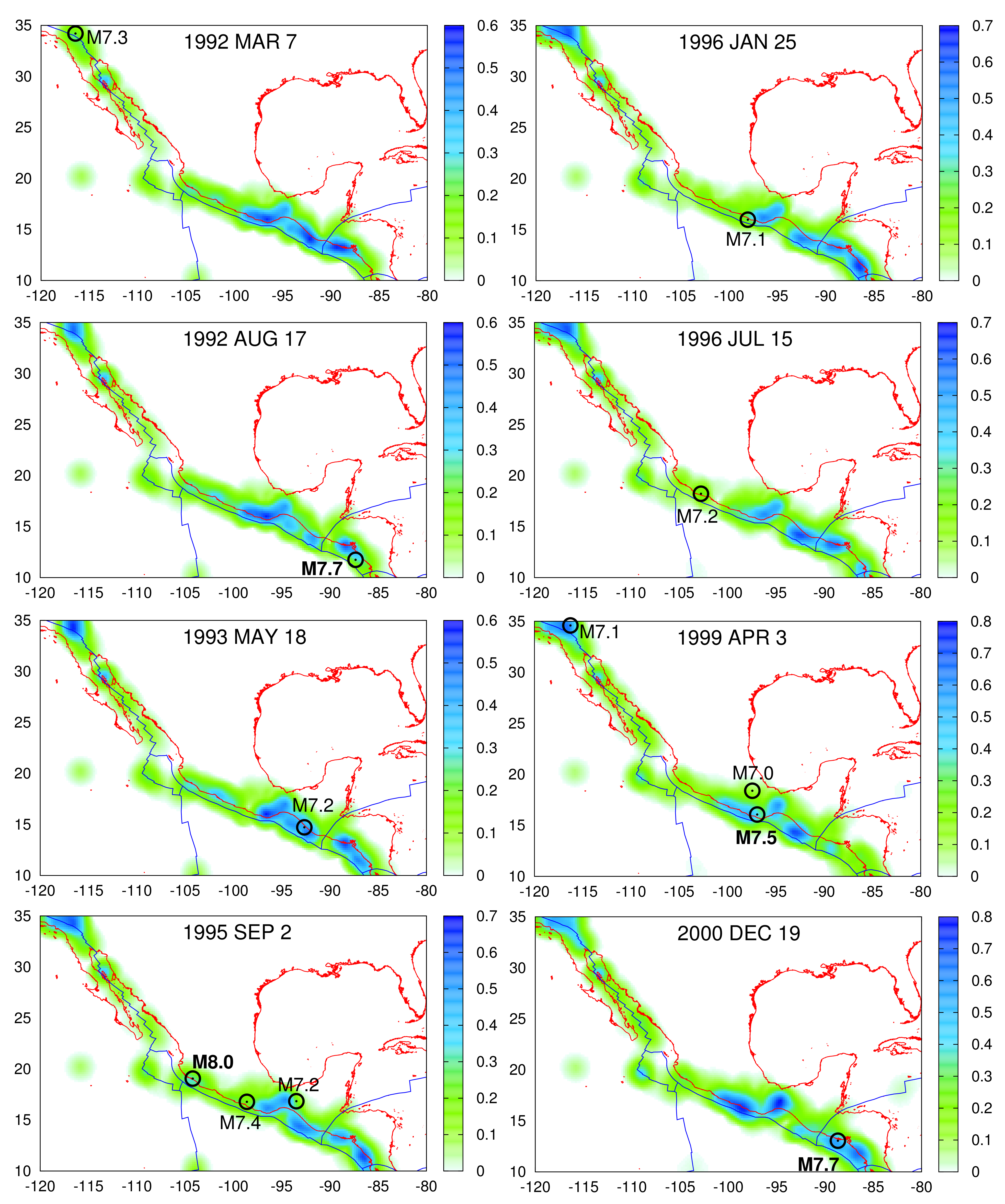
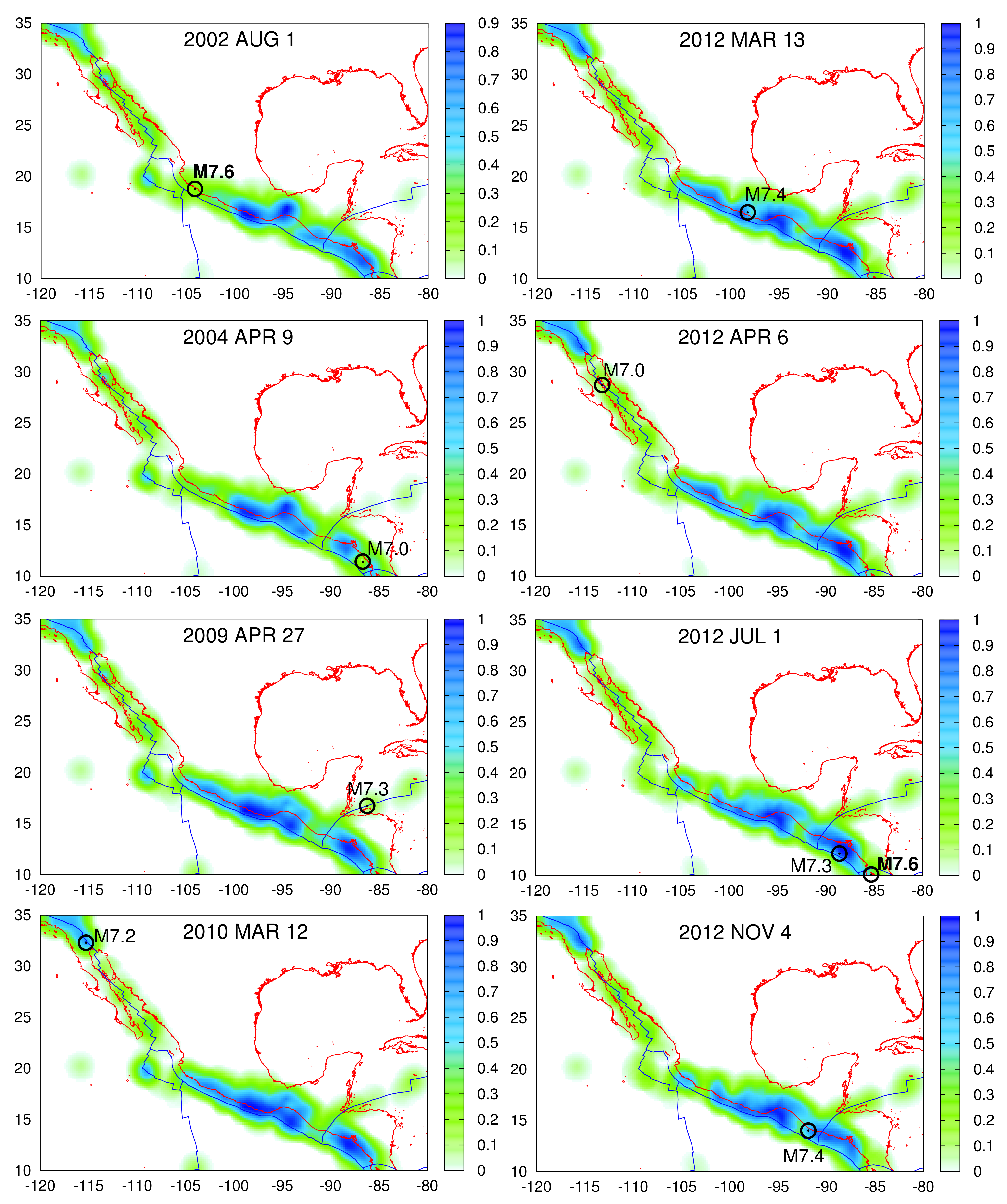
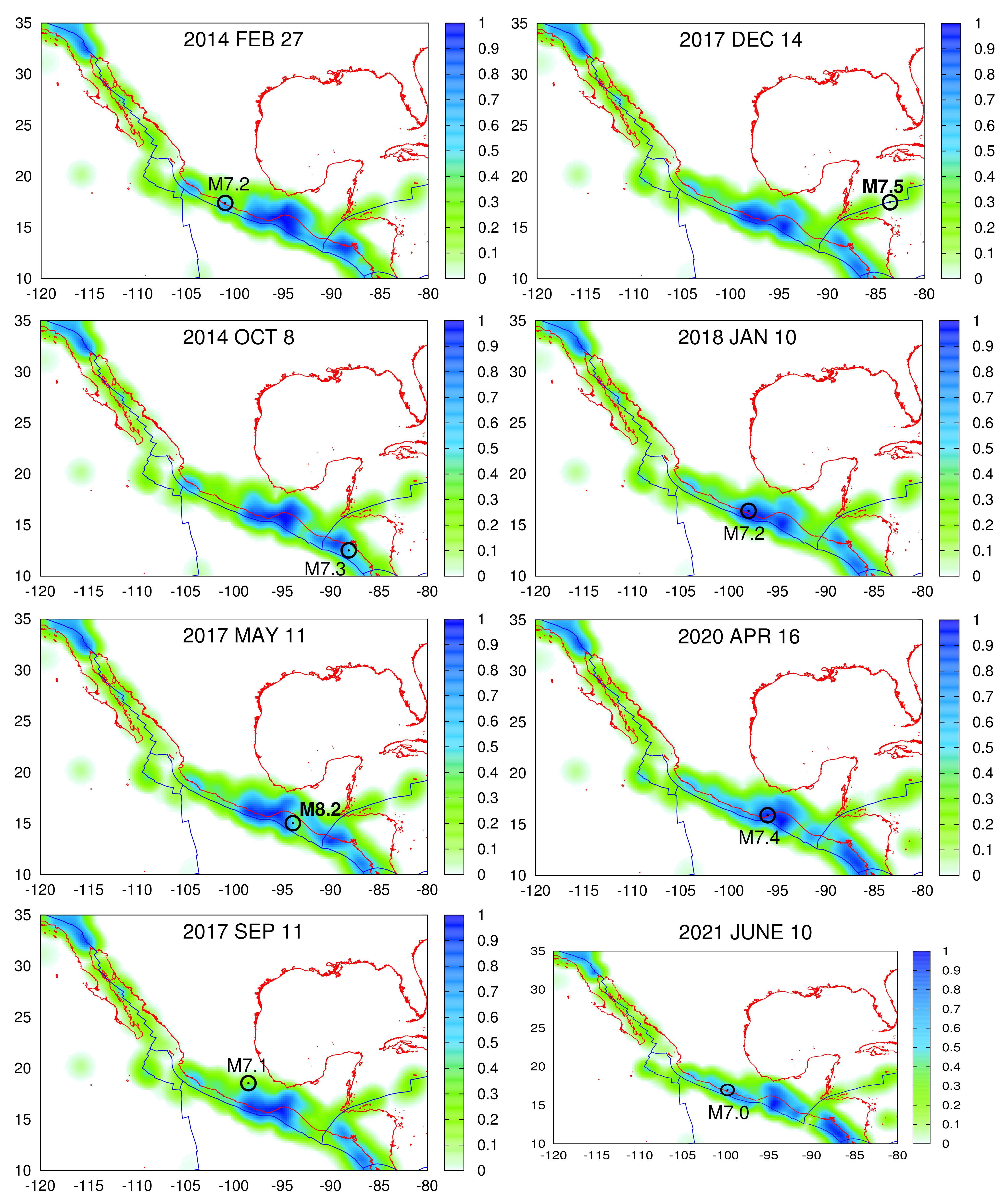
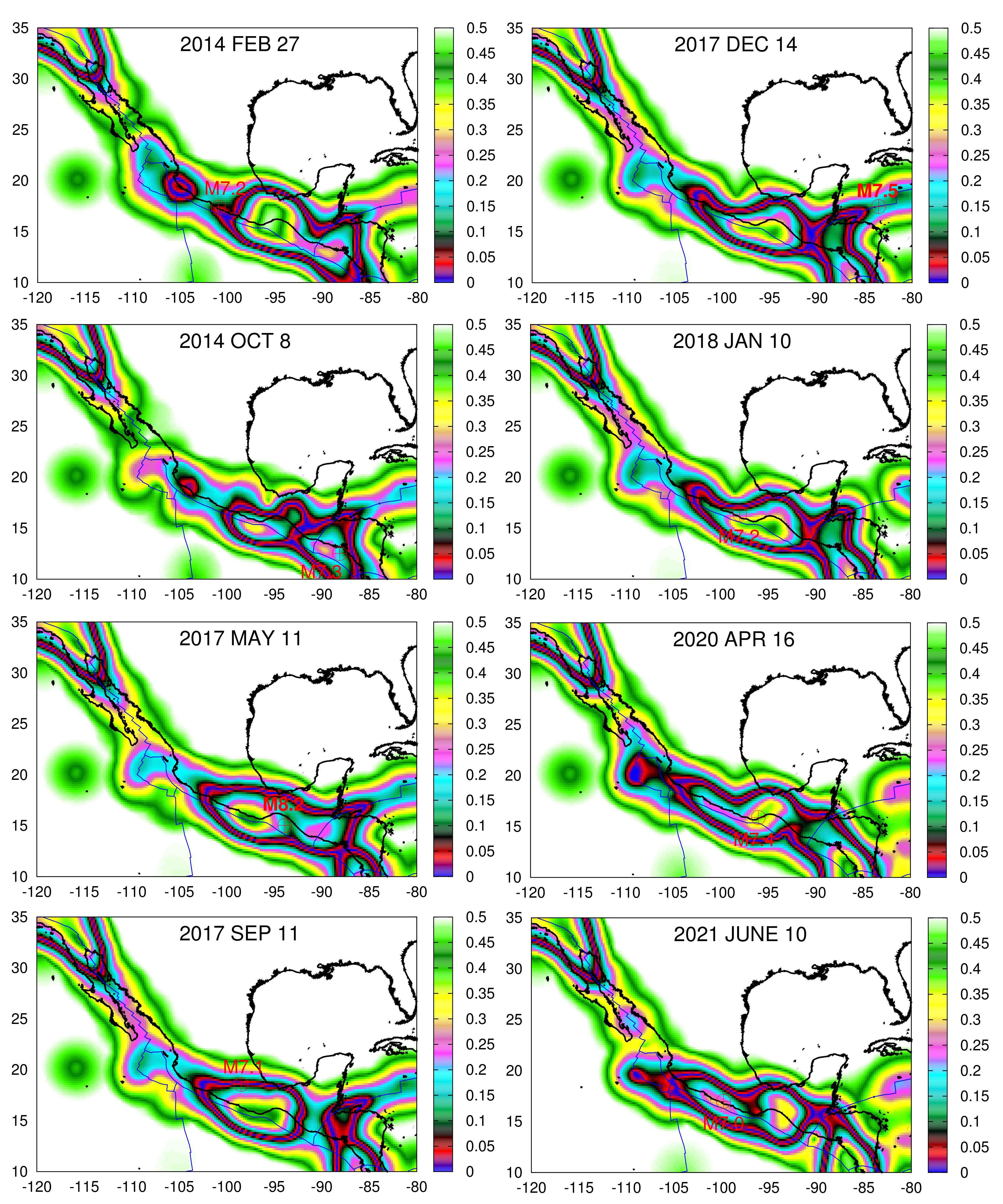
In Figure 5, using a 0.2 grid, we depict the ⟨EPS⟩ maps determined for R = 100 km for each date of Table 1 together with the location of the epicenters of the strong EQs that followed within the next six months. We observe that the EQ epicenters compare favorably with the contours of ⟨EPS⟩. This relation will be further elaborated in the next section.
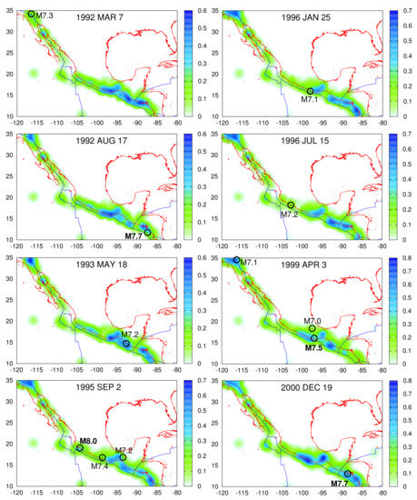
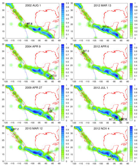
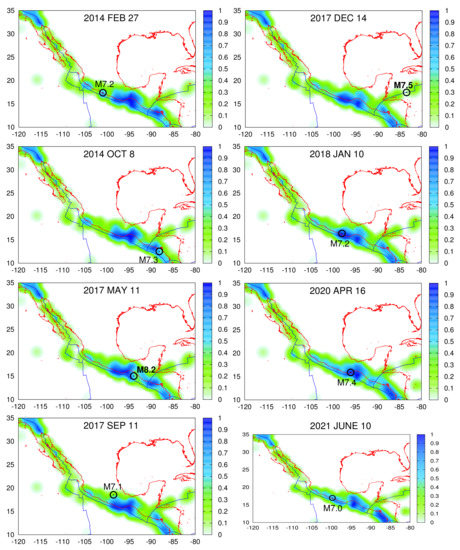
Figure 5.
Maps of the study area NW together with the plate boundaries (blue) according to Reference [73] depicting by color scale the ⟨EPS⟩ for R = 100 km at the dates of inserted in Table 1. The EQ epicenters are shown by the (black) open circles in each case and their magnitude is typed boldface when .
4. Discussion
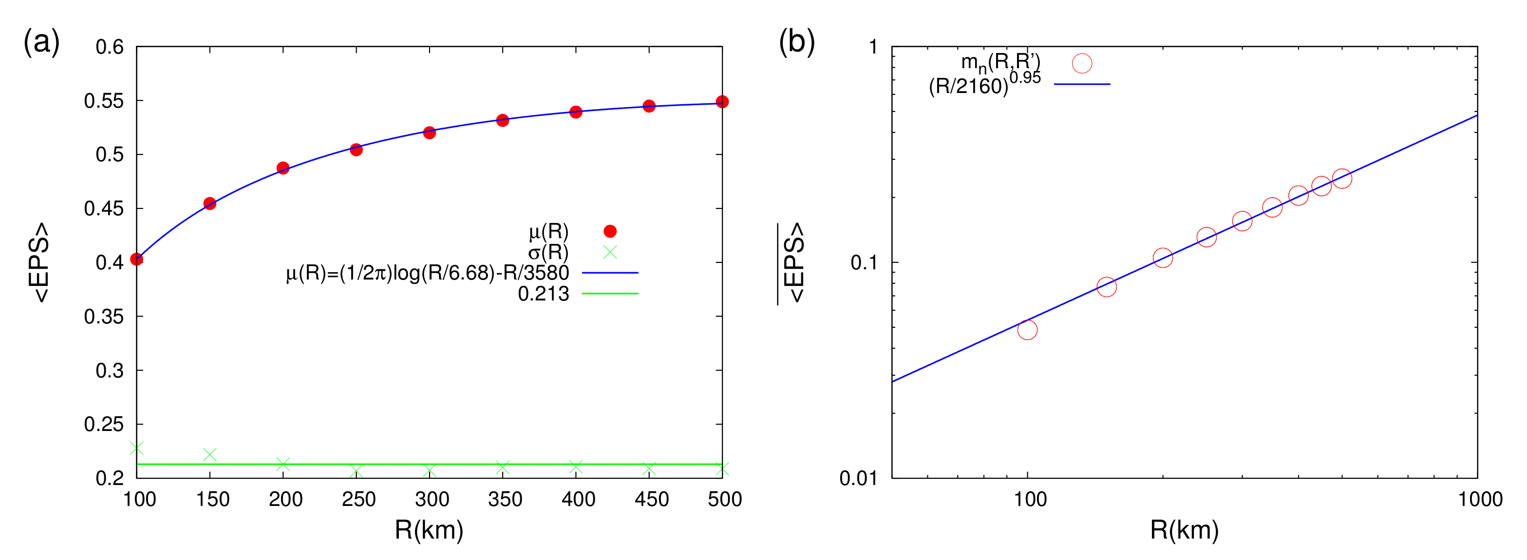
We first studied the statistics of the ⟨EPS⟩ values closest to the epicenters of the strong EQs with M during the period 1 January 1989 to 1 January 2021, i.e., the first 28 EQs of Table 1. The results for the mean value and the standard deviation (STD) are plotted versus R in Figure 6a, which indicates a characteristic behavior of a monotonically increasing . A further inspection of Figure 6a reveals that it is compatible with the functional form
which includes the characteristic logarithmic singular part of the Green’s function in two dimensions, see, e.g., Equation (9.96c) in paragraph 3 of Section 9.2.2.3 of Bronshtein et al. [104], together with a linear (non-singular) correction term. The presence of this singular logarithmic part when analyzing ⟨EPS⟩ closest to the strong EQ epicenters should be considered as a strong indication of the interrelation between the location of the epicenters and the corresponding ⟨EPS⟩ maps. It signifies that the future epicenters seem to act similar to sources in the two dimensional ⟨EPS⟩ field.

Figure 6.
Dependence of the ⟨EPS⟩ statistics on the coarse grain radius R: Panel (a) depicts the average value (red bullets) and the STD (green crosses) of the ⟨EPS⟩ values closest to each epicenter of the first 28 EQs of Table 1. The fitting function (blue) and the average value of (green horizontal line) are also shown. Panel (b) depicts the mean value over all the grid points of the ⟨EPS⟩ maps shown in all but the last panel of Figure 5. This mean value labeled (open red circles) is plotted vs. R together with the corresponding power law fit (blue straight line).
The above point is further strengthened by the fact that when considering the ⟨EPS⟩ mean value over all the lattice points of the grid (square lattice) for all the maps of Figure 5 that correspond to the first 28 EQs of Table 1 the singular behavior disappears, see Figure 6b. The functional form observed in Figure 6b indicates a value of = 0.95(2) which is compatible with the almost one-dimensional fault structure of Figure 1 (cf. the latter is dominated by the faults along the Pacific coast). Moreover, a comparison of Figure 6b with Equation (8) reveals that = 2160(80) km, which compares favorably with the quantity 2000 km when considering the study area A of 25.
Furthermore, we studied the statistics of ⟨EPS⟩ values closest to the epicenters of the 8 EQs with (shown with bold letters in Table 1 and Figure 5). It was found that for km, a particularly interesting behavior is observed: Namely a bimodal distribution appears with mean value 0.55 and two lobes ±0.15 from the mean. This, in conjunction with the fact that at km, Figure 6a reveals an average value of 0.50, encouraged us to investigate the maps of for values of R around 250 km (cf. in previous studies [19,58] km has also been found of particular importance). Such a study revealed that maps may be useful and the optimum results (shown in Figure 7) were obtained when using km.
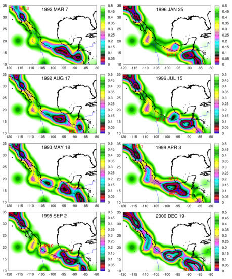
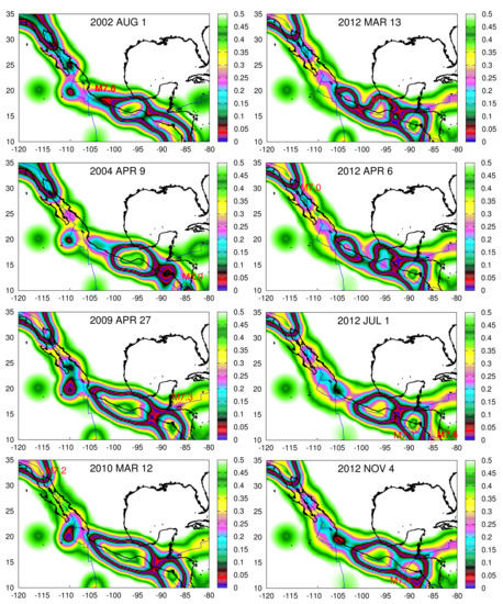
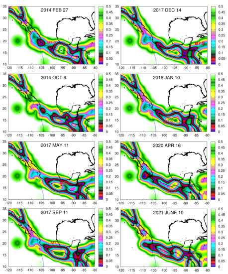
Figure 7.
Maps of the study area NW together with the plate boundaries (blue) according to Bird [73] depicting by color scale the quantity for R = 200 km at the dates of inserted in Table 1. The EQ epicenters are shown by the (red) circles with pluses in each case and their magnitude is typed boldface when .
An inspection of Figure 7 reveals that if we ignore the case of the 1997 Michoacan M7.2 EQ [105] that corresponds to the observed on 15 July 1996, the epicenters of all the other 28 strong EQs of magnitude M lie inside or up to 120 km away from the region shaded with tones of cyan color, i.e., with . This latter region on average covers only 8.5% of the total area with a STD of 2.3%. Additionally, 25 out of the 29 strong EQ epicenters of Table 1 lie within 65km away from the same region (cf. the 1993 M7.2, the 2012 M7.3, and the 2020 M7.4 EQs lie away 118 km, 87 km, and 115 km, respectively).
The results shown in Figure 7 do not, of course, solve the very difficult problem of finding the epicenter of a future strong EQ since the areas covered by the tones of cyan color are spatially distributed in a rather large area, but clearly indicate that ⟨EPS⟩ maps definitely include information concerning the epicenter of a future strong EQ. Our efforts to improve these results are in progress by applying this method to other seismically active areas around the globe (cf. the operation of SES measuring stations [106] is an essential factor for such an improvement since additional information on the future epicentral area can be thus obtained).
5. Conclusions
Here, we studied the variability of the order parameter of seismicity (introduced by natural time analysis) together with earthquake nowcasting within the highly active seismic region NW that covers Southern California, Mexico, and part of Central America. We suggest a self-consistent method of constructing ⟨EPS⟩ maps to obtain an estimation of the epicenter location of a future strong EQ of magnitude M in this region. The study of ⟨EPS⟩ values closest to the strong EQ epicenters showed a logarithmic behavior, which is reminiscent of the Green’s function in two dimensions. This is compatible with the view that the future epicenters act like ‘sources’ in these two dimensional maps. Using NTA and EN the epicenter of a future strong M EQ was estimated to lie in the vicinity of a region covering on average only 8.5% of the total study area with a hit rate 28/29(≈96.5%).
Author Contributions
Conceptualization, J.P.-O., P.K.V., E.S.S., and N.V.S.; methodology, J.P.-O., P.K.V., E.S.S., and N.V.S.; software, P.K.V., J.P.-O., and N.V.S.; validation, J.P.-O., P.K.V., and E.S.S.; formal analysis, J.P.-O., E.S.S., and N.V.S.; investigation, J.P.-O. and N.V.S.; resources, J.P.-O., E.S.S., and N.V.S.; data curation, J.P.-O. and N.V.S.; writing—original draft preparation, J.P.-O., P.K.V., E.S.S., and N.V.S.; writing—review and editing, J.P.-O., P.K.V., E.S.S., and N.V.S.; visualization, J.P.-O. and N.V.S.; supervision, E.S.S. and N.V.S.; project administration, N.V.S.; funding acquisition, J.P.-O. All authors have read and agreed to the published version of the manuscript.
Funding
This research received no external funding.
Data Availability Statement
Earthquake data come from the United States National Earthquake Information Center PDE and were downloaded from the United States Geological Survey, Earthquake HazardsProgram [84]. The last date the data were accessed was 21 September 2021. Gnuplot [107] was used for the preparation of the figures. The coast lines were imported from GEODAS Coastline Extractor [108]. The datasets generated during and/or analyzed during the current study are available from the corresponding author on reasonable request.
Acknowledgments
Jennifer Perez-Oregon deeply appreciates support from the National Council of Science and Technology (CONACYT) of Mexico (CVU No. 376516).
Conflicts of Interest
The authors declare no conflict of interest.
Abbreviations
The following abbreviations are used in this manuscript:
| CDF | Cumulative distribution function |
| EN | Earthquake nowcasting |
| ENBOSAP | Earthquake networks based on similar activity patterns |
| EPS | Earthquake potential score |
| EQ | Earthquake |
| M | magnitude |
| NEIC | National earthquake information center |
| NTA | Natural time analysis |
| PDE | Preliminary determination of epicenters |
| SES | Seismic electric signals |
| STD | Standard deviation |
| USGS | United States geological survey |
References
- Lowry, A.R.; Larson, K.M.; Kostoglodov, V.; Bilham, R. Transient fault slip in Guerrero, southern Mexico. Geophys. Res. Lett. 2001, 28, 3753–3756. [Google Scholar] [CrossRef] [Green Version]
- Pacheco, J.F.; Singh, S.K. Seismicity and state of stress in Guerrero segment of the Mexican subduction zone. J. Geophys. Res. Solid Earth 2010, 115, B01303. [Google Scholar] [CrossRef] [Green Version]
- Ramírez-Rojas, A.A.; Flores-Márquez, E. Order parameter analysis of seismicity of the Mexican Pacific coast. Phys. A 2013, 392, 2507–2512. [Google Scholar] [CrossRef]
- Flores-Márquez, E.L.; Ramírez-Rojas, A.; Perez-Oregon, J.; Sarlis, N.V.; Skordas, E.S.; Varotsos, P.A. Natural Time Analysis of Seismicity within the Mexican Flat Slab before the M7.1 Earthquake on 19 September 2017. Entropy 2020, 22, 730. [Google Scholar] [CrossRef]
- Varotsos, P.A.; Sarlis, N.V.; Skordas, E.S. Spatio-Temporal complexity aspects on the interrelation between Seismic Electric Signals and Seismicity. Pract. Athens Acad. 2001, 76, 294–321. [Google Scholar]
- Varotsos, P.A.; Sarlis, N.V.; Skordas, E.S. Long-range correlations in the electric signals that precede rupture. Phys. Rev. E 2002, 66, 011902. [Google Scholar] [CrossRef] [Green Version]
- Varotsos, P.A.; Sarlis, N.V.; Skordas, E.S. Natural Time Analysis: The New View of Time. Precursory Seismic Electric Signals, Earthquakes and Other Complex Time-Series; Springer: Berlin/Heidelberg, Germany, 2011. [Google Scholar] [CrossRef]
- Varotsos, P.A.; Sarlis, N.V.; Skordas, E.S.; Uyeda, S.; Kamogawa, M. Natural time analysis of critical phenomena. Proc. Natl. Acad. Sci. USA 2011, 108, 11361–11364. [Google Scholar] [CrossRef] [Green Version]
- Sarlis, N.V.; Skordas, E.S.; Varotsos, P.A.; Nagao, T.; Kamogawa, M.; Tanaka, H.; Uyeda, S. Minimum of the order parameter fluctuations of seismicity before major earthquakes in Japan. Proc. Natl. Acad. Sci. USA 2013, 110, 13734–13738. [Google Scholar] [CrossRef] [Green Version]
- Varotsos, P.A.; Sarlis, N.V.; Skordas, E.S. Self-organized criticality and earthquake predictability: A long-standing question in the light of natural time analysis. EPL (Europhys. Lett.) 2020, 132, 29001. [Google Scholar] [CrossRef]
- Rundle, J.B.; Turcotte, D.L.; Donnellan, A.; Grant Ludwig, L.; Luginbuhl, M.; Gong, G. Nowcasting earthquakes. Earth Space Sci. 2016, 3, 480–486. [Google Scholar] [CrossRef]
- Rundle, J.B.; Luginbuhl, M.; Giguere, A.; Turcotte, D.L. Natural Time, Nowcasting and the Physics of Earthquakes: Estimation of Seismic Risk to Global Megacities. Pure Appl. Geophys. 2018, 175, 647–660. [Google Scholar] [CrossRef] [Green Version]
- Luginbuhl, M.; Rundle, J.B.; Turcotte, D.L. Statistical physics models for aftershocks and induced seismicity. Philos. Trans. R. Soc. A 2018, 377, 20170397. [Google Scholar] [CrossRef] [Green Version]
- Luginbuhl, M.; Rundle, J.B.; Turcotte, D.L. Natural Time and Nowcasting Earthquakes: Are Large Global Earthquakes Temporally Clustered? Pure Appl. Geophys. 2018, 175, 661–670. [Google Scholar] [CrossRef]
- Rundle, J.B.; Giguere, A.; Turcotte, D.L.; Crutchfield, J.P.; Donnellan, A. Global Seismic Nowcasting With Shannon Information Entropy. Earth Space Sci. 2019, 6, 191–197. [Google Scholar] [CrossRef] [Green Version]
- Rundle, J.B.; Donnellan, A. Nowcasting Earthquakes in Southern California With Machine Learning: Bursts, Swarms, and Aftershocks May Be Related to Levels of Regional Tectonic Stress. Earth Space Sci. 2020, 7, e2020EA001097. [Google Scholar] [CrossRef]
- Rundle, J.; Stein, S.; Donnellan, A.; Turcotte, D.L.; Klein, W.; Saylor, C. The Complex Dynamics of Earthquake Fault Systems: New Approaches to Forecasting and Nowcasting of Earthquakes. Rep. Prog. Phys. 2021, 84, 076801. [Google Scholar] [CrossRef]
- Rundle, J.B.; Donnellan, A.; Fox, G.; Crutchfield, J.P. Nowcasting Earthquakes by Visualizing the Earthquake Cycle with Machine Learning: A Comparison of Two Methods. Surv. Geophys. 2021. [Google Scholar] [CrossRef]
- Varotsos, P.K.; Perez-Oregon, J.; Skordas, E.S.; Sarlis, N.V. Estimating the epicenter of an impending strong earthquake by combining the seismicity order parameter variability analysis with earthquake networks and nowcasting: Application in Eastern Mediterranean. Appl. Sci. 2021, 11, 10093. [Google Scholar] [CrossRef]
- Tenenbaum, J.N.; Havlin, S.; Stanley, H.E. Earthquake networks based on similar activity patterns. Phys. Rev. E 2012, 86, 046107. [Google Scholar] [CrossRef] [Green Version]
- Mintzelas, A.; Sarlis, N. Minima of the fluctuations of the order parameter of seismicity and earthquake networks based on similar activity patterns. Phys. A 2019, 527, 121293. [Google Scholar] [CrossRef]
- Sarlis, N.V.; Varotsos, P.A.; Skordas, E.S. Flux avalanches in YBa2Cu3O7-x films and rice piles: Natural time domain analysis. Phys. Rev. B 2006, 73, 054504. [Google Scholar] [CrossRef]
- Tsuji, D.; Katsuragi, H. Temporal analysis of acoustic emission from a plunged granular bed. Phys. Rev. E 2015, 92, 042201. [Google Scholar] [CrossRef] [Green Version]
- Ferre, J.; Barzegar, A.; Katzgraber, H.G.; Scalettar, R. Distribution of interevent avalanche times in disordered and frustrated spin systems. Phys. Rev. B 2019, 99, 024411. [Google Scholar] [CrossRef] [Green Version]
- Ramírez-Rojas, A.; Flores-Márquez, E.L.; Guzmán-Vargas, L.; Gálvez-Coyt, G.; Telesca, L.; Angulo-Brown, F. Statistical features of seismoelectric signals prior to M7.4 Guerrero-Oaxaca earthquake (México). Nat. Hazards Earth Syst. Sci. 2008, 8, 1001–1007. [Google Scholar] [CrossRef] [Green Version]
- Ramírez-Rojas, A.; Telesca, L.; Angulo-Brown, F. Entropy of geoelectrical time series in the natural time domain. Nat. Hazards Earth Syst. Sci. 2011, 11, 219–225. [Google Scholar] [CrossRef]
- Potirakis, S.M.; Karadimitrakis, A.; Eftaxias, K. Natural time analysis of critical phenomena: The case of pre-fracture electromagnetic emissions. Chaos 2013, 23, 023117. [Google Scholar] [CrossRef]
- Vallianatos, F.; Michas, G.; Benson, P.; Sammonds, P. Natural time analysis of critical phenomena: The case of acoustic emissions in triaxially deformed Etna basalt. Phys. A 2013, 392, 5172–5178. [Google Scholar] [CrossRef]
- Vallianatos, F.; Michas, G.; Papadakis, G. Non-extensive and natural time analysis of seismicity before the Mw6.4, October 12, 2013 earthquake in the South West segment of the Hellenic Arc. Phys. A 2014, 414, 163–173. [Google Scholar] [CrossRef]
- Potirakis, S.M.; Eftaxias, K.; Schekotov, A.; Yamaguchi, H.; Hayakawa, M. Criticality features in ultra-low frequency magnetic fields prior to the 2013 M6.3 Kobe earthquake. Ann. Geophys. 2016, 59, S0317. [Google Scholar] [CrossRef]
- Potirakis, S.M.; Asano, T.; Hayakawa, M. Criticality Analysis of the Lower Ionosphere Perturbations Prior to the 2016 Kumamoto (Japan) Earthquakes as Based on VLF Electromagnetic Wave Propagation Data Observed at Multiple Stations. Entropy 2018, 20, 199. [Google Scholar] [CrossRef] [Green Version]
- Yang, S.S.; Potirakis, S.M.; Sasmal, S.; Hayakawa, M. Natural Time Analysis of Global Navigation Satellite System Surface Deformation: The Case of the 2016 Kumamoto Earthquakes. Entropy 2020, 22, 674. [Google Scholar] [CrossRef] [PubMed]
- Vallianatos, F.; Michas, G.; Hloupis, G. Seismicity Patterns Prior to the Thessaly (Mw6.3) Strong Earthquake on 3 March 2021 in Terms of Multiresolution Wavelets and Natural Time Analysis. Geosciences 2021, 11, 379. [Google Scholar] [CrossRef]
- Ramírez-Rojas, A.; Flores-Márquez, E.L.; Sarlis, N.V.; Varotsos, P.A. The Complexity Measures Associated with the Fluctuations of the Entropy in Natural Time before the Deadly Mexico M8.2 Earthquake on 7 September 2017. Entropy 2018, 20, 477. [Google Scholar] [CrossRef] [PubMed] [Green Version]
- Hloupis, G.; Stavrakas, I.; Vallianatos, F.; Triantis, D. A preliminary study for prefailure indicators in acoustic emissions using wavelets and natural time analysis. Proc. Inst. Mech. Eng. Part L J. Mater. Des. Appl. 2016, 230, 780–788. [Google Scholar] [CrossRef]
- Niccolini, G.; Lacidogna, G.; Carpinteri, A. Fracture precursors in a working girder crane: AE natural-time and b-value time series analyses. Eng. Fract. Mech. 2019, 210, 393–399. [Google Scholar] [CrossRef]
- Loukidis, A.; Pasiou, E.D.; Sarlis, N.V.; Triantis, D. Fracture analysis of typical construction materials in natural time. Phys. A 2019, 547, 123831. [Google Scholar] [CrossRef]
- Niccolini, G.; Potirakis, S.M.; Lacidogna, G.; Borla, O. Criticality Hidden in Acoustic Emissions and in Changing Electrical Resistance during Fracture of Rocks and Cement-Based Materials. Materials 2020, 13, 5608. [Google Scholar] [CrossRef]
- Varotsos, C.A.; Tzanis, C. A new tool for the study of the ozone hole dynamics over Antarctica. Atmos. Environ. 2012, 47, 428–434. [Google Scholar] [CrossRef]
- Varotsos, C.A.; Tzanis, C.; Cracknell, A.P. Precursory signals of the major El Niño Southern Oscillation events. Theor. Appl. Climatol. 2016, 124, 903–912. [Google Scholar] [CrossRef]
- Varotsos, C.A.; Tzanis, C.G.; Sarlis, N.V. On the progress of the 2015–2016 El Niño event. Atmos. Chem. Phys. Discuss. 2015, 15, 35787–35797. [Google Scholar] [CrossRef] [Green Version]
- Varotsos, C.A.; Sarlis, N.V.; Efstathiou, M. On the association between the recent episode of the quasi-biennial oscillation and the strong El Niño event. Theor. Appl. Climatol. 2018, 133, 569–577. [Google Scholar] [CrossRef]
- Baldoumas, G.; Peschos, D.; Tatsis, G.; Chronopoulos, S.K.; Christofilakis, V.; Kostarakis, P.; Varotsos, P.; Sarlis, N.V.; Skordas, E.S.; Bechlioulis, A.; et al. A Prototype Photoplethysmography Electronic Device that Distinguishes Congestive Heart Failure from Healthy Individuals by Applying Natural Time Analysis. Electronics 2019, 8, 1288. [Google Scholar] [CrossRef] [Green Version]
- Baldoumas, G.; Peschos, D.; Tatsis, G.; Christofilakis, V.; Chronopoulos, S.K.; Kostarakis, P.; Varotsos, P.A.; Sarlis, N.V.; Skordas, E.S.; Bechlioulis, A.; et al. Remote sensing natural time analysis of heartbeat data by means of a portable photoplethysmography device. Int. J. Remote Sens. 2021, 42, 2292–2302. [Google Scholar] [CrossRef]
- Varotsos, P.A.; Sarlis, N.V.; Tanaka, H.K.; Skordas, E.S. Similarity of fluctuations in correlated systems: The case of seismicity. Phys. Rev. E 2005, 72, 041103. [Google Scholar] [CrossRef] [Green Version]
- Sarlis, N.V.; Skordas, E.S.; Varotsos, P.A. Multiplicative cascades and seismicity in natural time. Phys. Rev. E 2009, 80, 022102. [Google Scholar] [CrossRef] [Green Version]
- Sarlis, N.V.; Christopoulos, S.R.G. Natural time analysis of the Centennial Earthquake Catalog. Chaos 2012, 22, 023123. [Google Scholar] [CrossRef]
- Flores-Márquez, E.; Vargas, C.; Telesca, L.; Ramírez-Rojas, A. Analysis of the distribution of the order parameter of synthetic seismicity generated by a simple spring–block system with asperities. Phys. A 2014, 393, 508–512. [Google Scholar] [CrossRef]
- Sarlis, N.V.; Skordas, E.S.; Varotsos, P.A.; Ramírez-Rojas, A.; Flores-Márquez, E.L. Natural time analysis: On the deadly Mexico M8.2 earthquake on 7 September 2017. Phys. A 2018, 506, 625–634. [Google Scholar] [CrossRef]
- Loukidis, A.; Perez-Oregon, J.; Pasiou, E.D.; Sarlis, N.V.; Triantis, D. Similarity of fluctuations in critical systems: Acoustic emissions observed before fracture. Phys. A 2020, 566, 125622. [Google Scholar] [CrossRef]
- Sarlis, N.V.; Skordas, E.S.; Varotsos, P.A. Similarity of fluctuations in systems exhibiting Self-Organized Criticality. EPL (Europhys. Lett.) 2011, 96, 28006. [Google Scholar] [CrossRef]
- Olami, Z.; Feder, H.J.S.; Christensen, K. Self-organized criticality in a continuous, nonconservative cellular automaton modeling earthquakes. Phys. Rev. Lett. 1992, 68, 1244–1247. [Google Scholar] [CrossRef] [Green Version]
- Sarlis, N.V.; Skordas, E.S.; Varotsos, P.A. The change of the entropy in natural time under time-reversal in the Olami-Feder-Christensen earthquake model. Tectonophysics 2011, 513, 49–53. [Google Scholar] [CrossRef]
- Burridge, R.; Knopoff, L. Model and theoretical seismicity. Bull. Seismol. Soc. Am. 1967, 57, 341–371. [Google Scholar] [CrossRef]
- Varotsos, P.A.; Sarlis, N.V.; Skordas, E.S.; Uyeda, S.; Kamogawa, M. Natural time analysis of critical phenomena. The case of Seismicity. EPL 2010, 92, 29002. [Google Scholar] [CrossRef] [Green Version]
- Sarlis, N.V.; Skordas, E.S.; Varotsos, P.A. Order parameter fluctuations of seismicity in natural time before and after mainshocks. EPL 2010, 91, 59001. [Google Scholar] [CrossRef] [Green Version]
- Sarlis, N.V.; Christopoulos, S.R.G.; Skordas, E.S. Minima of the fluctuations of the order parameter of global seismicity. Chaos 2015, 25, 063110. [Google Scholar] [CrossRef] [Green Version]
- Sarlis, N.V.; Skordas, E.S.; Varotsos, P.A.; Nagao, T.; Kamogawa, M.; Uyeda, S. Spatiotemporal variations of seismicity before major earthquakes in the Japanese area and their relation with the epicentral locations. Proc. Natl. Acad. Sci. USA 2015, 112, 986–989. [Google Scholar] [CrossRef] [Green Version]
- Sarlis, N.V.; Skordas, E.S.; Varotsos, P.A.; Ramírez-Rojas, A.; Flores-Márquez, E.L. Identifying the Occurrence Time of the Deadly Mexico M8.2 Earthquake on 7 September 2017. Entropy 2019, 21, 301. [Google Scholar] [CrossRef] [PubMed] [Green Version]
- Sarlis, N.V.; Skordas, E.S.; Christopoulos, S.R.G.; Varotsos, P.A. Natural Time Analysis: The Area under the Receiver Operating Characteristic Curve of the Order Parameter Fluctuations Minima Preceding Major Earthquakes. Entropy 2020, 22, 583. [Google Scholar] [CrossRef] [PubMed]
- Christopoulos, S.R.G.; Skordas, E.S.; Sarlis, N.V. On the Statistical Significance of the Variability Minima of the Order Parameter of Seismicity by Means of Event Coincidence Analysis. Appl. Sci. 2020, 10, 662. [Google Scholar] [CrossRef] [Green Version]
- Skordas, E.S.; Christopoulos, S.R.G.; Sarlis, N.V. Detrended fluctuation analysis of seismicity and order parameter fluctuations before the M7.1 Ridgecrest earthquake. Nat. Hazards 2020, 100, 697–711. [Google Scholar] [CrossRef]
- Varotsos, P.A.; Sarlis, N.V.; Skordas, E.S.; Nagao, T.; Kamogawa, M. The unusual case of the ultra-deep 2015 Ogasawara earthquake (MW7.9): Natural time analysis. EPL 2021, 135, 49002. [Google Scholar] [CrossRef]
- Varotsos, P.; Alexopoulos, K.; Lazaridou, M. Latest aspects of earthquake prediction in Greece based on Seismic Electric Signals, II. Tectonophysics 1993, 224, 1–37. [Google Scholar] [CrossRef] [Green Version]
- Varotsos, P. The Physics of Seismic Electric Signals; TERRAPUB: Tokyo, Japan, 2005; p. 338. [Google Scholar]
- Varotsos, P.; Alexopoulos, K.; Nomicos, K. Seismic Electric Currents. Pract. Athens Acad. 1981, 56, 277–286. [Google Scholar]
- Varotsos, P.; Alexopoulos, K. Physical Properties of the variations of the electric field of the Earth preceding earthquakes, I. Tectonophysics 1984, 110, 73–98. [Google Scholar] [CrossRef]
- Varotsos, P.; Alexopoulos, K. Physical Properties of the variations of the electric field of the Earth preceding earthquakes, II. Tectonophysics 1984, 110, 99–125. [Google Scholar] [CrossRef]
- Varotsos, P.; Alexopoulos, K. Thermodynamics of Point Defects and Their Relation with Bulk Properties; North Holland: Amsterdam, The Netherlands, 1986. [Google Scholar] [CrossRef]
- Varotsos, P.; Lazaridou, M. Latest aspects of earthquake prediction in Greece based on Seismic Electric Signals. Tectonophysics 1991, 188, 321–347. [Google Scholar] [CrossRef]
- Varotsos, P.A.; Sarlis, N.V.; Skordas, E.S.; Lazaridou, M.S. Seismic Electric Signals: An additional fact showing their physical interconnection with seismicity. Tectonophysics 2013, 589, 116–125. [Google Scholar] [CrossRef]
- Skordas, E.; Sarlis, N. On the anomalous changes of seismicity and geomagnetic field prior to the 2011 9.0 Tohoku earthquake. J. Asian Earth Sci. 2014, 80, 161–164. [Google Scholar] [CrossRef]
- Bird, P. An updated digital model of plate boundaries. Geochem. Geophys. Geosyst. 2003, 4, 1027. [Google Scholar] [CrossRef]
- Rundle, J.B.; Luginbuhl, M.; Khapikova, P.; Turcotte, D.L.; Donnellan, A.; McKim, G. Nowcasting Great Global Earthquake and Tsunami Sources. Pure Appl. Geophys. 2020, 177, 359–368. [Google Scholar] [CrossRef]
- Luginbuhl, M.; Rundle, J.B.; Turcotte, D.L. Natural time and nowcasting induced seismicity at the Groningen gas field in the Netherlands. Geophys. J. Int. 2018, 215, 753–759. [Google Scholar] [CrossRef]
- Luginbuhl, M.; Rundle, J.B.; Hawkins, A.; Turcotte, D.L. Nowcasting Earthquakes: A Comparison of Induced Earthquakes in Oklahoma and at the Geysers, California. Pure Appl. Geophys. 2018, 175, 49–65. [Google Scholar] [CrossRef]
- Sarlis, N.V.; Skordas, E.S. Study in Natural Time of Geoelectric Field and Seismicity Changes Preceding the Mw6.8 Earthquake on 25 October 2018 in Greece. Entropy 2018, 20, 882. [Google Scholar] [CrossRef] [PubMed] [Green Version]
- Pasari, S. Nowcasting Earthquakes in the Bay of Bengal Region. Pure Appl. Geophys. 2019, 176, 1417–1432. [Google Scholar] [CrossRef]
- Pasari, S.; Sharma, Y. Contemporary Earthquake Hazards in the West-Northwest Himalaya: A Statistical Perspective through Natural Times. Seismol. Res. Lett. 2020, 91, 3358–3369. [Google Scholar] [CrossRef]
- Pasari, S.; Simanjuntak, A.V.H.; Neha; Sharma, Y. Nowcasting earthquakes in Sulawesi Island, Indonesia. Geosci. Lett. 2021, 8, 27. [Google Scholar] [CrossRef]
- Chouliaras, G. Investigating the earthquake catalog of the National Observatory of Athens. Nat. Hazards Earth Syst. Sci. 2009, 9, 905–912. [Google Scholar] [CrossRef]
- Chouliaras, G.; Melis, N.S.; Drakatos, G.; Makropoulos, K. Operational network improvements and increased reporting in the NOA (Greece) seismicity catalog. Adv. Geosci. 2013, 36, 7–9. [Google Scholar] [CrossRef] [Green Version]
- Mignan, A.; Chouliaras, G. Fifty Years of Seismic Network Performance in Greece (1964–2013): Spatiotemporal Evolution of the Completeness Magnitude. Seismol. Res. Lett. 2014, 85, 657–667. [Google Scholar] [CrossRef]
- United States Geological Survey, Earthquake Hazards Program. Search Earthquake Catalog. Available online: https://earthquake.usgs.gov/earthquakes/search/ (accessed on 21 September 2021).
- Dengo, G. Mid America: Tectonic setting for the Pacific margin from southern Mexico to northwestern Colombia. In The Ocean Basins and Margins; Springer: Boston, MA, USA, 1985; pp. 123–180. [Google Scholar] [CrossRef]
- Beavan, J.; Tregoning, P.; Bevis, M.; Kato, T.; Meertens, C. Motion and rigidity of the Pacific Plate and implications for plate boundary deformation. J. Geophys. Res. Solid Earth 2002, 107, 2261. [Google Scholar] [CrossRef]
- Anderson, T.H.; Schmidt, V.A. The evolution of Middle America and the Gulf of Mexico–Caribbean Sea region during Mesozoic time. Geol. Soc. Am. Bull. 1983, 94, 941–966. [Google Scholar] [CrossRef]
- Mooser, F. Provincias geotérmicas de México. Bol. Asoc. Mex. Geól. Pet. 1964, 16, 7–8. [Google Scholar]
- Luna, I.; Morrone, J.; Espinosa, D. Biodiversidad de la Faja Volcánica Transmexicana; Universidad Nacional Autónoma de México, Facultad de Estudios Superiores Zaragoza e Instituto de Biología: Mexico City, Mexico, 2007. [Google Scholar]
- Müller, R.D.; Sdrolias, M.; Gaina, C.; Roest, W.R. Age, spreading rates, and spreading asymmetry of the world’s ocean crust. Geochem. Geophys. Geosyst. 2008, 9, Q04006. [Google Scholar] [CrossRef]
- Pardo, M.; Suárez, G. Shape of the subducted Rivera and Cocos plates in southern Mexico: Seismic and tectonic implications. J. Geophys. Res. 1995, 100, 12357–12373. [Google Scholar] [CrossRef] [Green Version]
- Kim, Y.; Clayton, R.; Jackson, J. Geometry and seismic properties of the subducting Cocos plate in central Mexico. J. Geophys. Res. Solid Earth 2010, 115, B06310. [Google Scholar] [CrossRef] [Green Version]
- Alvarez, M. Tectónica profunda de México (in spanish). Bol. Asoc. Mex. Geól. Pet. 1958, 10, 163–182. [Google Scholar]
- Kanamori, H. Quantification of Earthquakes. Nature 1978, 271, 411–414. [Google Scholar] [CrossRef]
- Varotsos, P.A.; Sarlis, N.V.; Skordas, E.S. Study of the temporal correlations in the magnitude time series before major earthquakes in Japan. J. Geophys. Res. Space Phys. 2014, 119, 9192–9206. [Google Scholar] [CrossRef]
- Varotsos, P.A.; Sarlis, N.V.; Skordas, E.S. Scale-specific order parameter fluctuations of seismicity in natural time before mainshocks. EPL 2011, 96, 59002. [Google Scholar] [CrossRef] [Green Version]
- Rundle, J.B.; Donnellan, A.; Fox, G.; Crutchfield, J.P.; Granat, R. Nowcasting Earthquakes:Imaging the Earthquake Cycle in California with Machine Learning. Earth Space Sci. 2021, 8, e2021EA001757. [Google Scholar] [CrossRef]
- Perez-Oregon, J.; Angulo-Brown, F.; Sarlis, N.V. Nowcasting Avalanches as Earthquakes and the Predictability of Strong Avalanches in the Olami-Feder-Christensen Model. Entropy 2020, 22, 1228. [Google Scholar] [CrossRef]
- Ferguson, C.D.; Klein, W.; Rundle, J.B. Spinodals, scaling, and ergodicity in a threshold model with long-range stress transfer. Phys. Rev. E 1999, 60, 1359–1373. [Google Scholar] [CrossRef]
- Tiampo, K.F.; Rundle, J.B.; Klein, W.; Martins, J.S.S.; Ferguson, C.D. Ergodic Dynamics in a Natural Threshold System. Phys. Rev. Lett. 2003, 91, 238501. [Google Scholar] [CrossRef] [Green Version]
- Tiampo, K.F.; Rundle, J.B.; Klein, W.; Holliday, J.; Sá Martins, J.S.; Ferguson, C.D. Ergodicity in natural earthquake fault networks. Phys. Rev. E 2007, 75, 066107. [Google Scholar] [CrossRef] [Green Version]
- Press, W.H.; Teukolsky, S.; Vettrling, W.; Flannery, B.P. Numerical Recipes in FORTRAN; Cambridge Univrsity Press: New York, NY, USA, 1992; p. 963. [Google Scholar]
- Bak, P.; Christensen, K.; Danon, L.; Scanlon, T. Unified Scaling Law for Earthquakes. Phys. Rev. Lett. 2002, 88, 178501. [Google Scholar] [CrossRef] [Green Version]
- Bronshtein, I.; Semendyayev, K.; Musiol, G.; Mühlig, H. Handbook of Mathematics; Springer: Berlin/Heidelberg, Germany, 2007. [Google Scholar] [CrossRef]
- United States Geological Survey, Earthquake Hazards Program. M 7.2—46 km WNW of El Habillal, Mexico. Available online: https://earthquake.usgs.gov/earthquakes/eventpage/usp0007vrx/technical (accessed on 21 September 2021).
- Sarlis, N.V.; Varotsos, P.A.; Skordas, E.S.; Zlotnicki, J.; Nagao, T.; Rybin, A.; Lazaridou-Varotsos, M.S.; Papadopoulou, K. Seismic electric signals in seismic prone areas. Earthq. Sci. 2018, 31, 44–51. [Google Scholar] [CrossRef]
- Williams, T.; Kelley, C. Gnuplot 4.6: An Interactive Plotting Program. 2014. Available online: http://www.gnuplot.info (accessed on 28 February 2014).
- Metzger, D.R. GEODAS Coastline Extractor, Version 1.1.3.1. 2014. Available online: http://www.ngdc.noaa.gov/mgg/dat/geodas/software/mswindows/geodas-ng_setup.exe (accessed on 11 February 2015).


Publisher’s Note: MDPI stays neutral with regard to jurisdictional claims in published maps and institutional affiliations. |
© 2021 by the authors. Licensee MDPI, Basel, Switzerland. This article is an open access article distributed under the terms and conditions of the Creative Commons Attribution (CC BY) license (https://creativecommons.org/licenses/by/4.0/).