Abstract
We address the problem of unsupervised anomaly detection for multivariate data. Traditional machine learning based anomaly detection algorithms rely on specific assumptions of normal patterns and fail to model complex feature interactions and relations. Recently, existing deep learning based methods are promising for extracting representations from complex features. These methods train an auxiliary task, e.g., reconstruction and prediction, on normal samples. They further assume that anomalies fail to perform well on the auxiliary task since they are never trained during the model optimization. However, the assumption does not always hold in practice. Deep models may also perform the auxiliary task well on anomalous samples, leading to the failure detection of anomalies. To effectively detect anomalies for multivariate data, this paper introduces a teacher-student distillation based framework Distillated Teacher-Student Network Ensemble (DTSNE). The paradigm of the teacher-student distillation is able to deal with high-dimensional complex features. In addition, an ensemble of student networks provides a better capability to avoid generalizing the auxiliary task performance on anomalous samples. To validate the effectiveness of our model, we conduct extensive experiments on real-world datasets. Experimental results show superior performance of DTSNE over competing methods. Analysis and discussion towards the behavior of our model are also provided in the experiment section.
1. Introduction
Anomaly detection (a.k.a. outlier detection) [1,2] is referred to as detecting data points that significantly deviate from normal behaviors. Identifying anomalies for multivariate data always provides valuable information in various domains. For instance, anomalies in credit card transactions could imply online a fraud [3], while an unusual computer network traffic recording could signify unauthorized access [4]. Due to the great empirical value, efficient and accurate anomaly detection algorithms are desired.
Compared with normalities, anomalies are associated with unknownness, irregularity, and rarity [2]. Unknownness indicates that anomaly events can not be observed until they actually happen. Furthermore, irregularity means that the class structure of anomalies is highly heterogeneous. Last but not least, anomalies are rare in terms of collected data, leading to the problem of class imbalance. Due to the difficulty of collecting a large-scale labeled anomaly dataset, fully supervised methods are impractical in real-world scenarios. Unsupervised anomaly detection does not require labeled training data. However, they rely on assumptions on the distribution of data points. For example, several distance- and density-based approaches, e.g., Local Outlier Factor (LOF) [5], KNN (k-nearest neighbor) [6], and Isolation Forest (iForest) [7], assume that normalities reside in the high density area, whereas anomalies are far from the normal cluster. Probabilistic methods assume that normalities follow a specific distribution, e.g., ABOD (Angle-Based Outlier Detection) [8] and COPOD (Copula-Based Outlier Detection) [9]. Those methods fail to handle complex features because of high-dimensional features and sophisticated nonlinear relations.
Recently, a number of works have been introduced to improve anomaly detection by deep neural networks [2]. Deep learning [10] has had remarkable success in modeling intricate dependencies on a variety of domains. Instead of building assumptions of normality distribution, deep anomaly detection models the normal patterns by training networks via a surrogate task, such as reconstruction [11,12], prediction [13,14,15], and classification [16,17]. The underlying structure of normalities is captured through training a model on normal samples. It is intuitive that anomalies are expected to perform the surrogate task badly since they violate normal patterns learned by the model. However, existing deep anomaly detection methods are problematic for multivariate data. For instance, reconstruction-based methods are still ineffective since autoencoders tend to produce blurred reconstructions. Advanced generative models, e.g., generative adversarial nets [18], are promising to generate reliable reconstructions, whereas they suffer the difficulties of optimization. Prediction-based methods are predominantly designed for temporal data such as time-series and videos. Classification-based methods formulate the surrogate task as distinguishing the true type of a transformed image from different augmentations such as rotation, flipping, and cropping [16]. However, the augmentations require geometric structures contained in datasets, e.g., images and videos, which are impractical for multivariate data. Thus, a dedicated surrogate task is desired.
In this paper, we present a novel framework to achieve efficient and accurate anomaly detection. Novelties of this work are three fold. First, the framework of the teacher-student distillation is dedicatedly designed for multivariate data, enabling the capability to model complex feature interactions and relations. In addition, our proposed framework is general and can be extended to apply to other domains such as image anomaly detection and video anomaly detection. Second, the ensemble of student networks provides a capability to avoid potential generalizing of the auxiliary task on anomalous samples. Third, multiple anomaly scores are provided to detect anomalies from various aspects.
The paper is organized in the following order. Related works concerning state-of-the-art anomaly detection methods are reviewed in Section 2. Section 3 describes the overview of our proposed framework. In Section 4, a detailed description of the instantiated model of the framework is developed. The experimental setup, experimental results, and analysis are illustrated in Section 5. Finally, discussion and conclusions are presented in Section 6 and Section 7, respectively.
2. Related Work
There exists an abundance of works on unsupervised anomaly detection [2]. Traditional methods, such as LOF [5], SVDD (Support Vector Data Description) [19], and iForest [7], are ineffective at dealing with high-dimensional feature space or complex feature interactions. Although some works propose efficient techniques to deal with high-dimensional categorical feature’s interactions, e.g., CatBoost [20] and XGBoost [21], they are supervised methods and can not be directly applied on unsupervised anomaly detection. Deep anomaly detection (reviewed in [2]) becomes a vivid research area that includes various research topics such as utilizing prior knowledge [22,23] and representation learning for normalities [24,25]. However, unsupervised anomaly detection is still challenging due to the complexities of modeling nonlinear dependencies.
To tackle complex datasets, recent literature shows the trend of detecting anomalies via techniques including low-dimensional embedding, anomaly detector ensemble, and self-supervised pretext tasks.
2.1. Anomaly Detection via Low Dimensional Embedding
Performing anomaly detection on high-dimensional space is challenging since abnormal characteristics of anomalies are always invisible in an original space. A widely used solution is to reduce the dimension of original features where anomalies become noticeable in a reduced low-dimensional space. Traditional methods focusing on identifying anomalies in a subset of original features or a constructed subspace. These approaches can be categorized into two sub-categories, including subspace-based methods [26,27] and feature-selection based methods [28,29,30]. However, discovering complex feature interactions and couplings is still challenging for traditional algorithms. Recently, several methods leverage the power of deep learning and representation learning. REPEN, an instance of the framework RAMODO proposed in [24], combining with anomaly detection and representation learning, learns customized low-dimensional embeddings of ultrahigh-dimensional data for a random distance-based outlier detector. RDP [25] is a generic representation learning method by predicting data distances in a random projection space. By incorporating dedicated objectives, the low-dimensional representations obtained by RDP can be further used to perform various downstream tasks such as anomaly detection and clustering. Despite utilizing deep neural networks and representation learning, these methods learn representations and detect anomalies separately, which lead to indirect optimization and unstable performance.
2.2. Anomaly Detector Ensemble
Ensembling weak anomaly detectors into a strong anomaly detector is a powerful technique to achieve accurate anomaly detection. Traditional methods such as Feature Bagging [27], iForest [7], and LODA [31] try to combine outcomes from weak anomaly detectors to produce an ensembled anomaly score. However, these methods based on simple anomaly detectors and thus fail to model high-dimensional complex features.
2.3. Anomaly Detection with Self-Supervised Pretext Tasks
Recent self-supervised learning algorithms draw support from a pretext task to learn semantic representations. Different from representation learning, several methods utilize self-supervised pretext tasks to detect anomalies. GEOM [16] builds up a framework of self-supervised learning for anomaly detection. Specifically, GEOM applies multiple geometric transformations to an instance and trains a classifier to correctly predict the transformation giving a transformed instance. -Outlier [17] follows the idea of GEOM, adding up multiple anomaly scores. GOAD [32] substitutes the classification task in GEOM with a one-class classification task. However, the geometric transformations used in these methods require geometric structures contained in the dataset, which can not be directly applied to multivariate datasets.
3. The Distillation-Based Anomaly Detection Framework
3.1. Problem Statement
We address the problem of fully unsupervised anomaly detection for multivariate data. In detail, the framework consists of a triplet , where , , and stand for the model, the surrogate task, and the anomaly scoring function, respectively. By training the model via the surrogate task unsupervised and building the anomaly scoring function upon , the goal of anomaly detection is to assign anomaly scores to test samples in a way that we have , where is an anomaly and is a normal object.
Additionally, whether a test sample is an anomaly is judged by specifying an anomaly threshold :
where is the test result of .
3.2. The Proposed Framework
To tackle the problem of unsupervised anomaly detection, we introduce a novel framework including a teacher-student network and corresponding anomaly scores. In particular, the teacher network learns low-dimensional embeddings on the whole feature space, whereas only normal patterns are distillated from the teacher to student networks through a regression loss. Anomalies are highlighted by anomaly scores since gaps between the teacher network and student networks are expected to be large and uncertain. As shown in Figure 1, the framework contains three major modules:
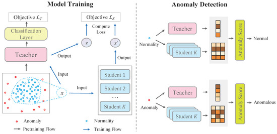
Figure 1.
Overview of our framework. The left-hand side illustrates the training procedure of the teacher network and student networks. The right-hand side shows the anomaly detection procedure.
- Teacher network is a parametric function that maps original features to low-dimensional vectors. We require the teacher network to have two properties. First, the teacher network is able to preserve the distance information of original space. Namely, two instances that are close in the original space are still close in the low-dimensional space. Second, the teacher network is a smooth and injective function such that the normality manifold is formed in the low-dimensional space, whereas anomalies are laid outside of the manifold.
- Student networks are a group of parametric functions . They are trained to mimic the outputs of the teacher network only on normal samples. All the students are independently trained to improve robustness. Anomalies are detected when the students fail to generalize the teacher mapping outside the normality manifold.
- Anomaly scores. By investigating the gaps between the teacher network and the student networks, we can define an anomaly score to identify anomalies. The anomalous samples are expected to gain larger gaps since only knowledge of normal patterns are distillated. In addition, the variance of students can be used as an additional criterion to detect anomalies.
To instantiate each component of the framework, we need to answer following questions:
- Q1: How can design the structure and the training objective of the teacher network be designed?
- Q2: How can the student networks be trained such that they mimic behaviors of the teacher only on normal samples?
- Q3: How can an anomaly score be defined that can effectively identify anomalous objects?
These questions are answered in Section 4.1, Section 4.2 and Section 4.3, respectively. Thus, we present an instantiated method of the framework called Distillated Teacher-Student Network Ensemble (DTSNE).
4. Distillated Teacher-Student Network Ensemble
4.1. Teacher Network for Low-Dimensional Embedding
Let be the original feature space where L is the dimension of . Normal samples lie in a subspace , whereas anomalous samples lie in a complementary space outside of the normal space . The teacher network that maps each instance in to a low-dimensional space (M is the dimensional of the low-dimensional space) is parameterized by weights . We implement the teacher network by a multi-layer neural network with ReLU [33] activation functions. Assuming that is a smooth injective mapping, low-dimensional representations of normal instances are expected to form a subspace where anomalies also lie in a complementary space . As described in Section 3.2, we require that the teacher network be able to map the normal instance to a normality manifold and meanwhile map the anomalous outside . To achieve this, the most direct way is to gather normal instances into a cluster and pull anomalous instances out when labels are available. However, this approach is infeasible under an unsupervised setting. Thus, we propose a self-supervised objective to discover the intrinsic regularities.
Pre-Training with Self-Supervised Pretext Tasks
Self-supervised methods learn semantic representations by applying a surrogate task such as context prediction [34], solving jigsaw puzzles [35], distinguishing image rotations [36], etc. In this paper, we present the learning objective as distinguishing instance augmentations. Like [16], multiple transformations are applied on each instance. The teacher network plus a classification layer is trained to predict the correct transformation of a given instance. The procedure is illustrated in Figure 2. In detail, we assume that the training dataset only contains normal samples (the problem of anomaly contamination is discussed in Section 4.3). We further use a group of affine transformations to transform the dataset:
where is the random weight matrix and is the random affine vector. Specifically, is an identity mapping when . Thus, the augmented dataset is given by:
where is an instance of the training dataset , and K is the number of transformations.
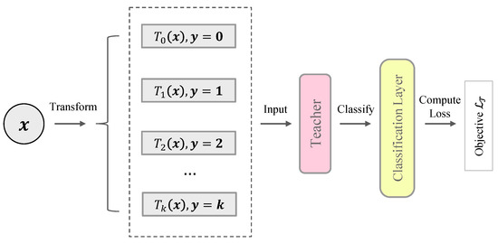
Figure 2.
Illustration of the teacher network pre-training. The pre-training means that we train the teacher network using a predefined objective before the main procedure of training student networks.
Conventional self-supervised learning always considers transformed instances belonging to the same semantic class. In contrast, we treat transformed instances as “pseudo-anomalies”, i.e., they do not belong to the normality manifold . Lastly, we design the training objective as distinguishing transformed instances. The probability that an instance is correctly classified is given by:
where is the Softmax function, and is a classification layer.
The final training objective of the teacher network is:
The pseudo-code of the teacher network pre-training is illustrated in Algorithm 1.
By distinguishing transformed instances, the representations that the teacher network produces are optimized to gather normal representations , whereas pull anomalous representations automatically in an unsupervised manner. In addition, we found that it also brings benefits to anomaly scoring. The details are discussed in Section 4.3:
| Algorithm 1 Teacher Network Pre-training |
| INPUT: Teacher network , training dataset , the number of transformation K |
| OUTPUT: Pre-trained teacher network |
|
A simplified version of the teacher network is just using Random Initialization without training. We show that Random Initialization is still capable of capturing internal regularities in the experimental section. Dedicated comparison of the two pre-training paradigms is conducted in Section 5.6. Kaiming Initialization [37] is used for the initialization strategy.
4.2. Distillated Students for Normality Learning
Now, we describe how to train student networks (, where N is the number of students) by utilizing the supervisory of the teacher network. All students are implemented by the same structure, a multi-layer neural network, and trained independently. The training objective contains two criterions. The first criterion is to optimize the instance-wise distance directly:
The second criterion is the pairwise distance that encapsulates pairwise similarity information:
For computation efficiency, the distance is measured by cosine similarity:
The final objective of student network training is given as:
where is a hyperparameter to adjust the weight of pairwise distance.
By only training on normal samples, the students manage to accurately regress the features solely for normal samples. They yield large regression errors and predictive uncertainties for anomalous samples.
4.3. Anomaly Scores for Anomaly Identification
In the evaluation phase, anomalous test samples are expected to receive larger gaps between the teacher network and student networks. The anomaly score measures how anomalous an instance is. In DTSNE, anomalies are identified by the anomaly score from two perspectives: closeness and uncertainties. Giving a predefined criterion , the closeness and the uncertainties are obtained by calculating the mean value and the variance over each students, respectively:
where is the weight of student variance.
To instantiate Equation (10), various dedicated anomaly scores can be defined. Specifically, a simple choice is the Mean Square Error (MSE):
In addition, advanced anomaly scores can be defined to utilize the information of self-supervised pre-training.
- Classification ProbabilitySince the teacher network is trained to distinguish different instance transformations, students are expected to perform the classification task well on normal samples. One can directly use the Softmax response as the anomaly score:This anomaly score measures the correctness of the student prediction giving each transformation of the instance .
- Cross EntropyFor each instance, we get K transformations in total. In addition, the k-th element of the Softmax response indicates the probability that the correct transformation index is k in terms of a transformed instance. Classification Probability (Equation (12)) only uses the k-th element of the Softmax response for the k-th transformation. To utilize information of all elements, we define the Cross Entropy based anomaly score:Here, the Cross Entropy measures the closeness of the Softmax response and the ground truth distribution.
- Information EntropySince student networks are trained to mimic the teacher network only on normal samples, we claim that the Softmax response of an anomalous sample is more chaotic than a normal sample’s. We can use Information Entropy to measure the prediction confidence:
In this paper, Mean Square Error and Information Entropy are used for anomaly scoring. Thus, the final anomaly score is given:
where is the weight of Information Entropy score.
Dealing with Anomaly Contamination
In Section 4.1, we assume that all the samples in the training dataset are normal, i.e., they are sampled from the normality manifold . However, this assumption is not guaranteed under an unsupervised scenario. This problem is called Anomaly Contamination. To alleviate this issue, we drop a portion of samples that have the highest anomaly scores per iteration to iteratively improve the pureness of the training dataset. This technique is also used in [25].
4.4. Summary
In summary, we propose the instantiation of our framework: DTSNE. The workflow contains three steps:
- Teacher network pre-training. First, the teacher network is first pre-trained with a self-supervised objective (Equation (5)) to learn underlying regularities of the data. In detail, we transform each instance using multiple random transformations and train the teacher network (plus a linear classification layer) to distinguish them. This objective helps the teacher network to produce better embeddings for downstream anomaly detection.
- Training of student networks. Second, the parameters of the teacher network are frozen. The teacher network can be treated as a function that provides supervision for students. Multiple student works are trained to mimic the outcomes of the teacher using the objective of Equation (9) only on normal samples.
- Anomaly scoring. Lastly, anomalies are identified by calculating an anomaly score. It evaluates the outcomes of students from a specific perspective, such as the difference between the teacher. In addition, we also use the uncertainties among students since they tend to produce contradictory outcomes for anomalous instances.
5. Experimental Results
5.1. Datasets
As shown in Table 1, the experiments are conducted on 10 publicly available datasets from various domains, including network intrusion detection, fraud detection, medical disease detection, etc. Two datasets contain real anomalies, including Lung and U2R, while other datasets are transformed from extremely imbalanced datasets. Following [22,25,38,39], the rare class in the imbalanced dataset is treated as semantically anomalies. Categorical features are encoded into discrete values via one-hot encoding. Lastly, all features are rescaled to the range using a min-max scaler to ensure the optimization efficiency.

Table 1.
Statistics of datasets.
5.2. Competing Methods
We consider various anomaly detection methods for evaluation, including traditional methods, e.g., LOF, outlier ensemble methods, e.g., iForest and LODA (Lightweight Online Detector of Anomalies), and state-of-the-art deep learning methods, e.g., DAGMM (Deep Autoencoding Gaussian Mixture Model) and RDP (Random Distance Prediction). The short descriptions of those methods are summarized as follows:
- iForest [7,40] is an outlier ensemble method that detects anomalies by selecting a random feature and then splits instances by a randomly selected splitting point into two subsets. The partitioning is applied recursively until a predefined termination condition is satisfied. Since the recursive partitioning can be represented by a binary tree structure, it is expected that anomalies have noticeably shorter paths started from the root node.
- LOF [5] is a density-based anomaly detection algorithm that detects anomalies by measuring the local deviation of a given instance w.r.t. its neighbors. The local deviation of an instance is given by the local density, which is calculated by the ratio of the KNN distance of the object to its k-nearest neighbors’ KNN distances. Under the assumption that anomalies lie in the low-density area, the local density of an anomaly is expected to be substantially lower than normal objects.
- LODA [31] is a lightweight ensemble system for anomaly detection. LODA groups weak anomaly detectors into a strong anomaly detector, which is robust to missing variables and identifying causes of anomalies.
- DAGMM [41] is composed of two modules, a deep autoencoder and a Gaussian Mixture Model (GMM). Instead of training the two components sequentially, DAGMM jointly optimizes the parameters of the two modules in an end-to-end fashion. This training strategy balances autoencoding reconstruction and density estimation of latent representations well, achieving a better capability of stable optimization and thus further reducing reconstruction errors.
- RDP [25] first trains a feature learner to predict data distances in a randomly projected space. The training process is flexible to incorporate auxiliary loss functions dedicatedly designed for downstream tasks such as anomaly detection and clustering. The representation learner is optimized to discover the intrinsic regularities of class structures that are implicitly embedded in the randomly projected space. Lastly, anomalies can be identified by calculating the distance between the representation learner and the random projection.
5.3. Implementation Details
This section provides the detailed information of our implementation. Since the evaluation focuses on multivariate data, multi-layer perceptrons (MLP) are used. Specifically, both the teacher network and the student network consist of two perceptron layers and a LeakyReLU activation function. In pre-training, the transformation matrices are sampled from Gaussian distribution. To perform classification, an additional classification layer is used, which is composed of a simple perceptron layer. In the training phase, the parameters of the teacher network are frozen. We use the SGD (Stochastic Gradient Descent) optimizer with momentum and L2 penalty. The learning rate, the momentum factor, and the L2 penalty factor are set as , , and , respectively. We apply gradient clipping to avoid overfitting, with a coefficient of . If self-supervised pre-training is enabled, we pre-train the teacher network using 100 epochs across all datasets. Furthermore, the student networks also trained using 100 epochs for each dataset.
5.4. Evaluation Metrics
Following related works [22,23,24,25], we focus on evaluating the score function instead of the test result (see Equation (1)). To achieve this, we use the area under the Receiver Operating Characteristic (ROC) curve, denoted as AUROC, and the mean Average Precision (mAP) as the performance metrics. In addition, all experiments are conducted at a virtual container with 32 GB dedicated memory, four Xeon CPU cores and four Geforce GTX 2080 GPU.
5.5. Parameter Settings
We choose the two factor (the weight of pairwise distance, in Equation (9)) and (the weight of student variance, in Equation (10)) empirically. Through quantitative experiments, we found the influence of and is very marginal when they are relatively small (see Section 5.7). To avoid over-parameterization, the two parameters are both set as 1 for simplification. Due to the two parameters: the number of students and the number of transformations significantly influence the computational efficiency, we empirically set them as 8 and 32, respectively. The portion of samples to be dropped is set as . We perform eight dropping iterations for the Apascal dataset and four iterations for other datasets. Other parameter settings such as batch size, embedding dimension, and are selected based on the dataset. Table 2 introduces the settings of them for each dataset respectively.
Table 2.
Parameter settings of different datasets. is the factor of the additional anomaly score (see Equation (15)).
5.6. Performance on Real-World Datasets
Experiment settings. This section compares the performance of DTSNE versus competing methods on real-world datasets. Each data set is first randomly split into two subsets, with instances as the training set and the other instances as the evaluation set. To ensure a reliable evaluation, 10 trials are independently performed with different random seeds. The performance is measured by AUROC and mAP scores. The implementations of iForest and LOF are taken from scikit-learn, a widely used machine learning library. All parameters of the two methods are set as default values. We implement LODA by APIs offered by PyOD [42], a comprehensive and scalable Python toolkit for anomaly detection. The parameters keep the default values from PyOD. DAGMM and RDP are implemented by PyTorch [43]. All the implementations of DAGMM and RDP and parameter settings are adopted from the code released with the original papers.
Analysis. The teacher-student distillation based framework enables DTSNE to achieve superior performance over competing methods. Table 3 and Table 4 report the AUROC scores and mAP scores, respectively (highest score highlighted in bold). In terms of AUROC scores, DTSNE achieves substantially better average performance than iForest (), LOF (), LODA (), DAGMM (), and RDP (); The improvements of our proposed method w.r.t. mAP scores is much more significant than iForest (), LOF (), LODA (), DAGMM (), and RDP (). These results show that our method can effectively deal with complex multivariate data. In detail, DTSNE outperforms LOF on all datasets w.r.t. both AUROC and mAP. This proves that simple density-based methods are ineffective in tackling complex feature interactions and relations. In addition, our proposed method also outperforms the two outlier-ensemble based methods, iForest and LODA, on all datasets. Compared with simply stacking weak anomaly detectors, our method utilizes multiple student networks and identifies anomalies from both the outcomes of student networks and disagreements among students. Lastly, DTSNE beats competing deep anomaly detection methods DAGMM and RDP as well. As for DAGMM, our method achieves better AUROC scores over all datasets and better mAP scores on almost all datasets except Secom. It has been proven that reconstruction-based anomaly detection is ineffective at dealing with multivariate data though deep neural networks that are used. In terms of RDP, DTSNE obtains better performance on almost all datasets. Instead of only investigating the gaps between the teacher and students, our method incorporates customized anomaly scores to leverage additional information contained in the outcomes of students. Except for that, the ensemble of student networks also contributes the improvements over RDP.
Table 3.
AUROC scores of DTSNE and baselines on 10 datasets. The best performance for each dataset is boldfaced.
Table 4.
mAP scores of DTSNE and baselines on 10 datasets. The best performance for each dataset is boldfaced.
Significance test. To investigate the significance of our proposed method, we perform a Friedman test [44] w.r.t. AUROC and mAP scores, respectively. A Friedman test is a non-parametric equivalent ANOVA (Analysis of variance) for multiple datasets. We further visualize the significance result in Figure 3. Two non-overlapping segments indicate “statistically difference” between the two algorithms. The test results suggest a significant difference between our method and baselines except RDP because a small overlap is observed. However, RDP is a state-of-the-art algorithm and the performance is already very high. We can still infer that DTSNE is much better than RDP since our method outperforms it on almost all datasets and the overlapping is extremely small.
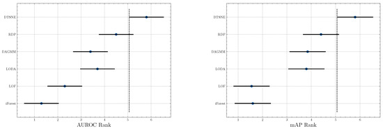
Figure 3.
Graphical presentation of the Friedman significance test w.r.t. AUROC and mAP scores.
5.7. Sensitivity Test w.r.t. Hyper-Parameters
Experiment settings. This section conducts the sensitivity test w.r.t. three perspectives: the representation dimension, the parameter , and the anomaly score. To empirically investigate the influence of them, we conduct quantitative experiments w.r.t. different settings on all datasets. The candidate values of the representation dimension are 4, 8, 16, 32, 64, 128, and 256, while the settings of include 0.1, 0.2, 0.5, 1, 2, 5, and 10.
Impact of representation dimensions.Figure 4 reports the AUROC scores and mAP scores of DTSNE w.r.t. different representation dimensions, respectively. The experimental results demonstrate the stability of our proposed method on different parameter settings across datasets. In terms of AUROC scores, the experimental results suggest that extremely large representation dimensions can not provide better performance. This illustrates that mapping original features into a high-dimensional representation space is not helpful for anomaly detection since anomalous patterns tend to be invisible in a higher-dimensional space. The experimental results also show extremely small representation dimensions can not provide sufficient information for the teacher network to learn a semantically rich representation. In terms of mAP scores, four datasets (AID362, Chess, CMC, and Secom) show flat trends in Figure 4. This suggest a good performance can be achieved with fairly small representation dimensions on the four datasets. Other datasets achieve best performance at a “elbow ” point. The settings of representation dimensions can be empirically selected as the “elbow” points to guarantee an accurate anomaly detection.
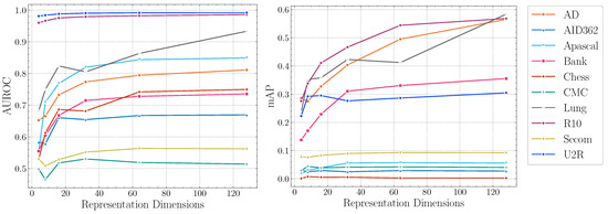
Figure 4.
AUROC and mAP scores of DTSNE w.r.t. representation dimensions.
Impact of .Figure 5 illustrates the influence of . The performance of DTSNE is relatively stable w.r.t. different values. When is extremely large, a rapid drop can be investigated for AD and R10 in terms of mAP scores. This phenomenon suggests to us to choose a relatively small value for . To avoid over-parameterization, we set as 1 for all datasets.
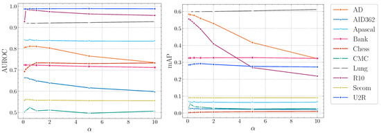
Figure 5.
AUROC and mAP scores of DTSNE w.r.t. different settings.
Impact of anomaly scores.Figure 6 and Figure 7 show the AUROC scores and mAP scores in terms of different anomaly scores separately. The experimental results suggest that none of the anomaly scores suppress others. Although Information Entropy and Classification Probability obtain improvement only in some cases, it never harms the performance. Cross Entropy performs worse on dataset AID362, Bank, and Lung, but it also achieves improvements on dataset Apascal, CMC, and Secom. To summarize, the choice of anomaly scores heavily relies on characteristics of datasets. In this paper, we use Information Entropy as the additional anomaly score since it performs stably on all datasets.
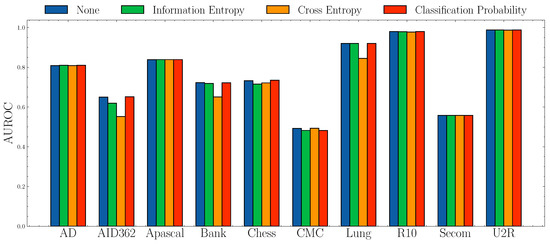
Figure 6.
AUROC socres w.r.t. different anomaly scores.
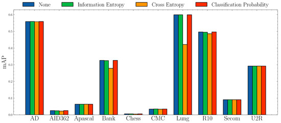
Figure 7.
mAP socres w.r.t. different anomaly scores.
5.8. Ablation Study
Experiment settings. In this section, we examine the effectiveness of the key component of DTSNE, self-supervised pre-training, by comparing the performance of random initialization and self-supervised pre-training. The variant is called , where the self-supervised pre-training is disabled. The teacher network of is randomly initialized without training. The network structure and training settings of DTSNE and its variants are totally the same.
Analysis. The experimental results show the importance of applying self-supervised pre-training for the teacher network. Table 5 shows the performance of DTSNE and its variant. Specifically, DTSNE boosts up AUROC scores () and mAP scores (), respectively, than variants. As discussed in Section 4.1, the reason for such improvement is that self-supervised pre-training enables our model to preserve intrinsic regularities of the normal manifold, which makes anomalies more noticeable in the representation space simultaneously. The experimental results also show that the technique is widely applicable on various datasets since they are collected from different domains with different dimensions (ranging from tens to thousands). Moreover, it is also noticeable that the variant obtains favorable results on most of the datasets. This phenomenon suggests that a random smooth function to some extent has the ability to reflect interactions from the original space. More discussion can be found in [25].
Table 5.
AUROC scores and mAP scores of DTSNE variants.
6. Discussion
Anomaly Detection in Low-dimensional Embedding. Detecting anomalies in a reduced space is a widely used solution to tackle high-dimensional complex feature space. In this paper, the reasons for learning low-dimensional representations are two fold: first, in contrast to operating on original space, detecting anomalies on low-dimensional space. Second, one can assume that normal data points are lying inside the normality manifold, whereas anomalies are lying outside. By mapping data points into a lower dimensional compact space, regularities are preserved while irregularities are highlighted.
Self-supervised Pre-training. Compared with using a random projection like [25], we pre-train the teacher network with a self-supervised objective. Though a random projection implemented by a neural network has some good properties with such smoothness, the ability to preserve the normal manifold can not be guaranteed without any regularization, which may potentially map anomalies into an area close to the normal cluster. As a result, the self-supervised pre-training is thus an essential component in DTSNE. We believe the importance of using self-supervised pre-training is also true in other anomaly detection algorithms.
Ensemble of Weak Anomaly Detectors. Conventional ensemble anomaly detection aims at effectively aggregating detection results from weak anomaly detectors. Different from that, our ensemble approach considers an additional perspective: uncertainties of weak anomaly detectors (namely students). Diversities among students are guaranteed by different initialization states. Since knowledge about anomalies is not accessible during the training phase, the uncertainties among weak anomaly detectors is an important sign to identify anomalous instances. This technique is readily applicable to other ensemble-based anomaly detection algorithms.
7. Conclusions
In this paper, we proposed a teacher-student distillation based anomaly detection framework and a corresponding instantiation DTSNE (Distillated Teacher-Student Network Ensemble). Key components including self-supervised pre-training, teacher-student distillation, student ensemble, and multiple anomaly scores enable DTSNE to greatly outperform state-of-the-art anomaly detection algorithms. The effectiveness of our method to detect anomalies for multivariate data is justified by extensive experiments. DTSNE achieves a substantially better average performance and than RDP (a state-of-the-art anomaly detection method) in terms of AUROC scores and mAP scores, respectively. The experimental results imply broader impacts of our techniques: self-supervised pre-training and student ensemble.
8. Future Work
The proposed approach achieves promising performance for unsupervised anomaly detection on various real-world datasets. The success suggests to us to explore future works on refining the current framework. One of the drawbacks of our approach is that the improvements of additional anomaly scores are not significant. The reason is that the information provided by outcomes of students is not fully utilized. To make the best use of information of the outcomes, we propose that the future work could look at developing a criteria to measure the uncertainties of student networks instead of only using variance. Similar works in recent literature, such as Bayesian Neural Networks [45] and Predictive Uncertainty [46], can provide inspiration to achieve the goal.
Furthermore, the future work could be explored on incorporating partial available labels. It is natural to occasionally obtain some annotations in real-world applications. As recent literature [23,47] suggests, only partial labels can significantly improve the performance of anomaly detection compared to a fully unsupervised scenario. Therefore, future work needs to extend our framework to adopt the semi-supervised setting.
Author Contributions
Conceptualization, Q.X., J.W., and Y.L.; methodology, Q.X. and J.W.; software, Q.X., G.H., and W.G.; validation, M.L. and F.W.; formal analysis, M.L. and F.W.; investigation, J.W., M.L., and F.W.; resources, J.W. and Y.L.; data curation, J.W. and Y.L.; writing—original draft preparation, Q.X.; writing—review and editing, J.W.; visualization, Q.X. and W.G.; supervision, J.W. and Y.L.; project administration, Y.L.; funding acquisition, J.W. All authors have read and agreed to the published version of the manuscript.
Funding
This research was funded by the Program of the Co-Construction with the Beijing Municipal Commission of Education of China Grant No. B19H100010, B18H100040, and K19H100010.
Institutional Review Board Statement
Not applicable.
Informed Consent Statement
Not applicable.
Data Availability Statement
No new data were created or analyzed in this study. Data sharing is not applicable to this article.
Conflicts of Interest
The authors declare no conflict of interest. The funders had no role in the design of the study; in the collection, analyses, or interpretation of data; in the writing of the manuscript, or in the decision to publish the results.
References
- Aggarwal, C.C. Outlier Analysis, 2nd ed.; Springer Publishing Company, Incorporated: New York, NY, USA, 2016. [Google Scholar]
- Pang, G.; Shen, C.; Cao, L.; van den Hengel, A. Deep Learning for Anomaly Detection: A Review. arXiv 2020, arXiv:2007.02500. [Google Scholar]
- Pourhabibi, T.; Ong, K.; Kam, B.; Boo, Y.L. Fraud detection: A systematic literature review of graph-based anomaly detection approaches. Decis. Support Syst. 2020, 133, 113303. [Google Scholar] [CrossRef]
- Tang, X.; Li, W.; Shen, J.; Qi, F.; Guo, S. Traffic Anomaly Detection for Data Communication Networks. In Proceedings of the 6th International Conference on Artificial Intelligence and Security (ICAIS), Hohhot, China, 17–20 July 2020; Lecture Notes in Computer, Science. Sun, X., Wang, J., Bertino, E., Eds.; Springer: New York, NY, USA, 2020; Volume 12240, pp. 440–450. [Google Scholar] [CrossRef]
- Breunig, M.M.; Kriegel, H.; Ng, R.T.; Sander, J. LOF: Identifying Density-Based Local Outliers. In Proceedings of the 2000 ACM SIGMOD International Conference on Management of Data, Dallas, TX, USA, 16–18 May 2000; Chen, W., Naughton, J.F., Bernstein, P.A., Eds.; ACM: New York, NY, USA, 2000; pp. 93–104. [Google Scholar] [CrossRef]
- Ramaswamy, S.; Rastogi, R.; Shim, K. Efficient Algorithms for Mining Outliers from Large Data Sets. In Proceedings of the 2000 ACM SIGMOD International Conference on Management of Data, Dallas, TX, USA, 16–18 May 2000; Chen, W., Naughton, J.F., Bernstein, P.A., Eds.; ACM: New York, NY, USA, 2000; pp. 427–438. [Google Scholar] [CrossRef]
- Liu, F.T.; Ting, K.M.; Zhou, Z. Isolation Forest. In Proceedings of the 8th IEEE International Conference on Data Mining (ICDM 2008), Pisa, Italy, 15–19 December 2008; pp. 413–422. [Google Scholar] [CrossRef]
- Kriegel, H.; Schubert, M.; Zimek, A. Angle-based outlier detection in high-dimensional data. In Proceedings of the 14th ACM SIGKDD International Conference on Knowledge Discovery and Data Mining, Las Vegas, NV, USA, 24–27 August 2008; Li, Y., Liu, B., Sarawagi, S., Eds.; ACM: New York, NY, USA, 2008; pp. 444–452. [Google Scholar] [CrossRef]
- Li, Z.; Zhao, Y.; Botta, N.; Ionescu, C.; Hu, X. COPOD: Copula-Based Outlier Detection. arXiv 2020, arXiv:2009.09463. [Google Scholar]
- LeCun, Y.; Bengio, Y.; Hinton, G. Deep learning. Nature 2015, 521, 436–444. [Google Scholar] [CrossRef] [PubMed]
- Zenati, H.; Romain, M.; Foo, C.; Lecouat, B.; Chandrasekhar, V. Adversarially Learned Anomaly Detection. In Proceedings of the IEEE International Conference on Data Mining (ICDM 2018), Singapore, 17–20 November 2018; pp. 727–736. [Google Scholar] [CrossRef]
- Pidhorskyi, S.; Almohsen, R.; Doretto, G. Generative Probabilistic Novelty Detection with Adversarial Autoencoders. In Advances in Neural Information Processing Systems 31: Proceedings of the Annual Conference on Neural Information Processing Systems 2018 (NeurIPS 2018), Montréal, QC, Canada, 3–8 December 2018; Bengio, S., Wallach, H.M., Larochelle, H., Grauman, K., Cesa-Bianchi, N., Garnett, R., Eds.; Curran Associates Inc.: Red Hook, NY, USA, 2018; pp. 6823–6834. [Google Scholar]
- Liu, W.; Luo, W.; Lian, D.; Gao, S. Future Frame Prediction for Anomaly Detection—A New Baseline. In Proceedings of the 2018 IEEE Conference on Computer Vision and Pattern Recognition (CVPR 2018), Salt Lake City, UT, USA, 18–22 June 2018; pp. 6536–6545. [Google Scholar] [CrossRef]
- Abati, D.; Porrello, A.; Calderara, S.; Cucchiara, R. Latent Space Autoregression for Novelty Detection. In Proceedings of the IEEE Conference on Computer Vision and Pattern Recognition (CVPR 2019), Long Beach, CA, USA, 16–20 June 2019; pp. 481–490. [Google Scholar] [CrossRef]
- Ye, M.; Peng, X.; Gan, W.; Wu, W.; Qiao, Y. AnoPCN: Video Anomaly Detection via Deep Predictive Coding Network. In Proceedings of the 27th ACM International Conference on Multimedia (MM 2019), Nice, France, 21–25 October 2019; Amsaleg, L., Huet, B., Larson, M.A., Gravier, G., Hung, H., Ngo, C., Ooi, W.T., Eds.; ACM: New York, NY, USA, 2019; pp. 1805–1813. [Google Scholar] [CrossRef]
- Golan, I.; El-Yaniv, R. Deep Anomaly Detection Using Geometric Transformations. In Advances in Neural Information Processing Systems 31: Proceedings of the Annual Conference on Neural Information Processing Systems 2018 (NeurIPS 2018), Montréal, QC, Canada, 3–8 December 2018; Bengio, S., Wallach, H.M., Larochelle, H., Grauman, K., Cesa-Bianchi, N., Garnett, R., Eds.; Curran Associates Inc.: Red Hook, NY, USA, 2018; pp. 9781–9791. [Google Scholar]
- Wang, S.; Zeng, Y.; Liu, X.; Zhu, E.; Yin, J.; Xu, C.; Kloft, M. Effective End-to-end Unsupervised Outlier Detection via Inlier Priority of Discriminative Network. In Advances in Neural Information Processing Systems 32: Proceedings of the Annual Conference on Neural Information Processing Systems 2019 (NeurIPS 2019), Vancouver, BC, Canada, 8–14 December 2019; Wallach, H.M., Larochelle, H., Beygelzimer, A., d’Alché-Buc, F., Fox, E.B., Garnett, R., Eds.; Curran Associates Inc.: Red Hook, NY, USA, 2019; pp. 5960–5973. [Google Scholar]
- Goodfellow, I.J.; Pouget-Abadie, J.; Mirza, M.; Xu, B.; Warde-Farley, D.; Ozair, S.; Courville, A.C.; Bengio, Y. Generative Adversarial Nets. In Advances in Neural Information Processing Systems 27: Proceedings of the Annual Conference on Neural Information Processing Systems 2014, Montreal, QC, Canada, 8–13 December 2014; Ghahramani, Z., Welling, M., Cortes, C., Lawrence, N.D., Weinberger, K.Q., Eds.; Curran Associates Inc.: Red Hook, NY, USA, 2014; pp. 2672–2680. [Google Scholar]
- Tax, D.M.J.; Duin, R.P.W. Support vector domain description. Pattern Recognit. Lett. 1999, 20, 1191–1199. [Google Scholar] [CrossRef]
- Prokhorenkova, L.O.; Gusev, G.; Vorobev, A.; Dorogush, A.V.; Gulin, A. CatBoost: Unbiased boosting with categorical features. In Advances in Neural Information Processing Systems 31: Proceedings of the Annual Conference on Neural Information Processing Systems 2018 (NeurIPS 2018), Montréal, QC, Canada, 3–8 December 2018; Bengio, S., Wallach, H.M., Larochelle, H., Grauman, K., Cesa-Bianchi, N., Garnett, R., Eds.; Curran Associates Inc.: Red Hook, NY, USA, 2018; pp. 6639–6649. [Google Scholar]
- Chen, T.; Guestrin, C. XGBoost: A Scalable Tree Boosting System. In Proceedings of the 22nd ACM SIGKDD International Conference on Knowledge Discovery and Data Mining, San Francisco, CA, USA, 13–17 August 2016; Krishnapuram, B., Shah, M., Smola, A.J., Aggarwal, C.C., Shen, D., Rastogi, R., Eds.; ACM: New York, NY, USA, 2016; pp. 785–794. [Google Scholar] [CrossRef]
- Pang, G.; Shen, C.; van den Hengel, A. Deep Anomaly Detection with Deviation Networks. In Proceedings of the 25th ACM SIGKDD International Conference on Knowledge Discovery & Data Mining (KDD 2019), Anchorage, AK, USA, 4–8 August 2019; Teredesai, A., Kumar, V., Li, Y., Rosales, R., Terzi, E., Karypis, G., Eds.; ACM: New York, NY, USA, 2019; pp. 353–362. [Google Scholar] [CrossRef]
- Pang, G.; van den Hengel, A.; Shen, C. Weakly-supervised Deep Anomaly Detection with Pairwise Relation Learning. arXiv 2019, arXiv:1910.13601. [Google Scholar]
- Pang, G.; Cao, L.; Chen, L.; Liu, H. Learning Representations of Ultrahigh-dimensional Data for Random Distance-based Outlier Detection. In Proceedings of the 24th ACM SIGKDD International Conference on Knowledge Discovery & Data Mining (KDD 2018), London, UK, 19–23 August 2018; Guo, Y., Farooq, F., Eds.; ACM: New York, NY, USA, 2018; pp. 2041–2050. [Google Scholar] [CrossRef]
- Wang, H.; Pang, G.; Shen, C.; Ma, C. Unsupervised Representation Learning by Predicting Random Distances. In Proceedings of the Twenty-Ninth International Joint Conference on Artificial Intelligence (IJCAI 2020), Yokohama, Japan, 11–17 July 2020; Bessiere, C., Ed.; 2020; pp. 2950–2956. [Google Scholar] [CrossRef]
- Keller, F.; Müller, E.; Böhm, K. HiCS: High Contrast Subspaces for Density-Based Outlier Ranking. In Proceedings of the IEEE 28th International Conference on Data Engineering (ICDE 2012), Arlington, VA, USA, 1–5 April 2012; Kementsietsidis, A., Salles, M.A.V., Eds.; IEEE Computer Society: Washington, DC, USA, 2012; pp. 1037–1048. [Google Scholar] [CrossRef]
- Lazarevic, A.; Kumar, V. Feature bagging for outlier detection. In Proceedings of the Eleventh ACM SIGKDD International Conference on Knowledge Discovery and Data Mining, Chicago, IL, USA, 21–24 August 2005; Grossman, R., Bayardo, R.J., Bennett, K.P., Eds.; ACM: New York, NY, USA, 2005; pp. 157–166. [Google Scholar] [CrossRef]
- Azmandian, F.; Yilmazer, A.; Dy, J.G.; Aslam, J.A.; Kaeli, D.R. GPU-Accelerated Feature Selection for Outlier Detection Using the Local Kernel Density Ratio. In Proceedings of the 12th IEEE International Conference on Data Mining (ICDM 2012), Brussels, Belgium, 10–13 December 2012; Zaki, M.J., Siebes, A., Yu, J.X., Goethals, B., Webb, G.I., Wu, X., Eds.; IEEE Computer Society: Washington, DC, USA, 2012; pp. 51–60. [Google Scholar] [CrossRef]
- Pang, G.; Cao, L.; Chen, L.; Lian, D.; Liu, H. Sparse Modeling-Based Sequential Ensemble Learning for Effective Outlier Detection in High-Dimensional Numeric Data. In Proceedings of the Thirty-Second AAAI Conference on Artificial Intelligence (AAAI-18), the 30th Innovative Applications of Artificial Intelligence (IAAI-18), and the 8th AAAI Symposium on Educational Advances in Artificial Intelligence (EAAI-18), New Orleans, LA, USA, 2–7 February 2018; McIlraith, S.A., Weinberger, K.Q., Eds.; AAAI Press: Palo Alto, CA, USA, 2018; pp. 3892–3899. [Google Scholar]
- Pang, G.; Cao, L.; Chen, L.; Liu, H. Learning Homophily Couplings from Non-IID Data for Joint Feature Selection and Noise-Resilient Outlier Detection. In Proceedings of the Twenty-Sixth International Joint Conference on Artificial Intelligence (IJCAI 2017), Melbourne, Australia, 19–25 August 2017; Sierra, C., Ed.; 2017; pp. 2585–2591. [Google Scholar] [CrossRef]
- Pevný, T. Loda: Lightweight on-line detector of anomalies. Mach. Learn. 2016, 102, 275–304. [Google Scholar] [CrossRef]
- Bergman, L.; Hoshen, Y. Classification-Based Anomaly Detection for General Data. In Proceedings of the 8th International Conference on Learning Representations (ICLR 2020), Addis Ababa, Ethiopia, 26–30 April 2020. [Google Scholar]
- Maas, A.L.; Hannun, A.Y.; Ng, A.Y. Rectifier nonlinearities improve neural network acoustic models. In Proceedings of the 30th International Conference on Machine Learning, Atlanta, GA, USA, 16–21 June 2013; Volume 30, p. 3. [Google Scholar]
- Doersch, C.; Gupta, A.; Efros, A.A. Unsupervised Visual Representation Learning by Context Prediction. In Proceedings of the 2015 IEEE International Conference on Computer Vision (ICCV 2015), Santiago, Chile, 7–13 December 2015; pp. 1422–1430. [Google Scholar] [CrossRef]
- Noroozi, M.; Favaro, P. Unsupervised Learning of Visual Representations by Solving Jigsaw Puzzles. In Proceedings of the 14th European Conference on Computer Vision (ECCV 2016), Amsterdam, The Netherlands, 11–14 October 2016; Part VI, Lecture Notes in Computer Science. Leibe, B., Matas, J., Sebe, N., Welling, M., Eds.; Springer: New York, NY, USA, 2016; Volume 9910, pp. 69–84. [Google Scholar] [CrossRef]
- Gidaris, S.; Singh, P.; Komodakis, N. Unsupervised Representation Learning by Predicting Image Rotations. In Proceedings of the 6th International Conference on Learning Representations (ICLR 2018), Vancouver, BC, Canada, 30 April–3 May 2018. [Google Scholar]
- He, K.; Zhang, X.; Ren, S.; Sun, J. Delving Deep into Rectifiers: Surpassing Human-Level Performance on ImageNet Classification. In Proceedings of the 2015 IEEE International Conference on Computer Vision (ICCV 2015), Santiago, Chile, 7–13 December 2015; pp. 1026–1034. [Google Scholar] [CrossRef]
- Pang, G.; Cao, L.; Chen, L. Outlier Detection in Complex Categorical Data by Modeling the Feature Value Couplings. In Proceedings of the Twenty-Fifth International Joint Conference on Artificial Intelligence (IJCAI 2016), New York, NY, USA, 9–15 July 2016; Kambhampati, S., Ed.; IJCAI/AAAI Press: Palo Alto, CA, USA, 2016; pp. 1902–1908. [Google Scholar]
- Pang, G.; Cao, L.; Chen, L.; Liu, H. Unsupervised Feature Selection for Outlier Detection by Modelling Hierarchical Value-Feature Couplings. In Proceedings of the IEEE 16th International Conference on Data Mining (ICDM 2016), Barcelona, Spain, 12–15 December 2016; Bonchi, F., Domingo-Ferrer, J., Baeza-Yates, R., Zhou, Z., Wu, X., Eds.; IEEE Computer Society: Washington, DC, USA, 2016; pp. 410–419. [Google Scholar] [CrossRef]
- Liu, F.T.; Ting, K.M.; Zhou, Z. Isolation-Based Anomaly Detection. ACM Trans. Knowl. Discov. Data 2012, 6, 3:1–3:39. [Google Scholar] [CrossRef]
- Zong, B.; Song, Q.; Min, M.R.; Cheng, W.; Lumezanu, C.; Cho, D.; Chen, H. Deep Autoencoding Gaussian Mixture Model for Unsupervised Anomaly Detection. In Proceedings of the 6th International Conference on Learning Representations (ICLR 2018), Vancouver, BC, Canada, 30 April–3 May 2018. [Google Scholar]
- Zhao, Y.; Nasrullah, Z.; Li, Z. PyOD: A Python Toolbox for Scalable Outlier Detection. J. Mach. Learn. Res. 2019, 20, 96:1–96:7. [Google Scholar]
- Paszke, A.; Gross, S.; Massa, F.; Lerer, A.; Bradbury, J.; Chanan, G.; Killeen, T.; Lin, Z.; Gimelshein, N.; Antiga, L.; et al. PyTorch: An Imperative Style, High-Performance Deep Learning Library. In Advances in Neural Information Processing Systems 32: Proceedings of the Annual Conference on Neural Information Processing Systems 2019 (NeurIPS 2019), Vancouver, BC, Canada, 8–14 December 2019; Wallach, H.M., Larochelle, H., Beygelzimer, A., d’Alché-Buc, F., Fox, E.B., Garnett, R., Eds.; Curran Associates Inc.: Red Hook, NY, USA, 2019; pp. 8024–8035. [Google Scholar]
- Demsar, J. Statistical Comparisons of Classifiers over Multiple Data Sets. J. Mach. Learn. Res. 2006, 7, 1–30. [Google Scholar]
- Malinin, A.; Gales, M.J.F. Predictive Uncertainty Estimation via Prior Networks. In Advances in Neural Information Processing Systems 31: Proceedings of the Annual Conference on Neural Information Processing Systems 2018 (NeurIPS 2018), Montréal, QC, Canada, 3–8 December 2018; Bengio, S., Wallach, H.M., Larochelle, H., Grauman, K., Cesa-Bianchi, N., Garnett, R., Eds.; Curran Associates Inc.: Red Hook, NY, USA, 2018; pp. 7047–7058. [Google Scholar]
- Snoek, J.; Ovadia, Y.; Fertig, E.; Lakshminarayanan, B.; Nowozin, S.; Sculley, D.; Dillon, J.V.; Ren, J.; Nado, Z. Can you trust your model’s uncertainty? Evaluating predictive uncertainty under dataset shift. In Advances in Neural Information Processing Systems 32: Proceedings of the Annual Conference on Neural Information Processing Systems 2019(NeurIPS 2019), Vancouver, BC, Canada, 8–14 December 2019; Wallach, H.M., Larochelle, H., Beygelzimer, A., d’Alché-Buc, F., Fox, E.B., Garnett, R., Eds.; Curran Associates Inc.: Red Hook, NY, USA, 2019; pp. 13969–13980. [Google Scholar]
- Ruff, L.; Vandermeulen, R.A.; Görnitz, N.; Binder, A.; Müller, E.; Müller, K.; Kloft, M. Deep Semi-Supervised Anomaly Detection. In Proceedings of the 8th International Conference on Learning Representations (ICLR 2020), Addis Ababa, Ethiopia, 26–30 April 2020. [Google Scholar]


Publisher’s Note: MDPI stays neutral with regard to jurisdictional claims in published maps and institutional affiliations. |
© 2021 by the authors. Licensee MDPI, Basel, Switzerland. This article is an open access article distributed under the terms and conditions of the Creative Commons Attribution (CC BY) license (http://creativecommons.org/licenses/by/4.0/).