Abstract
The transverse momentum spectra of charged pions, kaons, and protons produced at mid-rapidity in central nucleus–nucleus (AA) collisions at high energies are analyzed by considering particles to be created from two participant partons, which are assumed to be contributors from the collision system. Each participant (contributor) parton is assumed to contribute to the transverse momentum by a Tsallis-like function. The contributions of the two participant partons are regarded as the two components of transverse momentum of the identified particle. The experimental data measured in high-energy AA collisions by international collaborations are studied. The excitation functions of kinetic freeze-out temperature and transverse flow velocity are extracted. The two parameters increase quickly from ≈3 to ≈10 GeV (exactly from 2.7 to 7.7 GeV) and then slowly at above 10 GeV with the increase of collision energy. In particular, there is a plateau from near 10 GeV to 200 GeV in the excitation function of kinetic freeze-out temperature.
Keywords:
excitation functions of related parameters; participant parton; kinetic freeze-out temperature; transverse flow velocity PACS:
12.40.Ee, 13.85.Hd, 24.10.Pa
1. Introduction
High-energy collider experiments are designed to study the strongly interacting matter at high temperatures and densities [1]. The deconfinement of colliding hadrons into quark-gluon plasma (QGP), which then rapidly expands and cools down [2], is conjectured to be created at such extreme collision energies [3,4,5,6]. In high-energy and nuclear physics, the study of transverse (momentum () or mass ()) spectra of charged particles produced in nucleus–nucleus (AA) collisions is very important. In particular, the AA collision process at the Relativistic Heavy Ion Collider (RHIC) and the Large Hadron Collider (LHC) provides a good opportunity to study the signals and characteristics of QGP generation, so as to indirectly study the system evolution and the reaction mechanism of particle generation.
During the time evolution of collision system [7,8,9], the stages of kinetic freeze-out and chemical freeze-out are two important processes. In the stage of chemical freeze-out, a phase transition from QGP to hadrons occurred in the system, so the composition and ratio of various particles remain unchanged. In the stage of kinetic freeze-out, elastic collisions among particles stop, so their and then spectra are unchanged [8,10]. Therefore, by studying the () spectra, we can obtain some useful information, such as the effective temperature (T), the chemical freeze-out temperature (), and the kinetic freeze-out temperature ( or ) of the system, as well as the transverse flow velocity () of the final state particles. The temperature in which we do not exclude the contribution of transverse flow is called the effective temperature, which is related to the kinetic freeze-out temperature. The temperatures in the stages of chemical and kinetic freeze-outs are called the chemical and kinetic freeze-out temperatures, respectively.
It is very important to study the behavior of and due to their relation to map the phase diagram of Quantum Chromodynamics (QCD), though is usually used [11,12,13,14,15,16] in the phase diagram. In order to extract and , and study their dependence on energy, we can analyze the () spectra of particles using different models. These models include, but are not limited to, the blast-wave model with Boltzmann–Gibbs statistics [17,18] or Tsallis statistics [19,20,21], as well as other alternative methods [22,23,24,25,26] based on the standard distribution or Tsallis distribution. Here, the standard distribution denotes together the Boltzmann, Fermi–Dirac, and Bose–Einstein distributions. The alternative method regards the intercept of T versus as , and the slope of versus as , where , , and denote the rest mass, mean , and mean energy of the given particles, respectively.
In our recent work [27,28], the blast-wave model with Boltzmann–Gibbs statistics or Tsallis statistics and the standard distribution have been used to analyze the spectra of particles produced in high-energy proton–proton (pp) and AA collisions. The related parameters were extracted and their excitation functions were obtained. Not only the blast-wave model [17,18,19,20,21], but also the alternative method [22,23,24,25,26], can be used to extract and , though an effective temperature T is used in the latter. The alternative method is partly a new one, in which the extractions of both and are based on T [22,23,29] and the related derived quantities such as and .
Due to the importance of and and their excitation functions, we use a new method in the framework of multisource thermal model [30] to describe the () spectra of identified particles in this work. Considering the contributions of two participant (contributor) partons to of a given particle, we regard the two contributions as the two components of . The () spectra of identified particles (concretely charged pions, kaons, and protons) produced at mid-rapidity (mid-y) in central AA collisions which include gold–gold (Au-Au) collisions at the Alternating Gradient Synchrotron (AGS), lead–lead (Pb-Pb) collisions at the Super Proton Synchrotron (SPS), Au–Au collisions at the RHIC, and Pb–Pb and xenon–xenon (Xe-Xe) collisions at the LHC are studied. The center-of-mass energy per nucleon pair, , considered by us is from 2.7 GeV to 5.44 TeV. After fitting the experimental data measured by the E866 [31], E895 [32,33], E802 [34,35], NA49 [36,37], STAR [38,39,40], and ALICE Collaborations [41,42,43], we analyze the tendency of parameters.
2. Formalism and Method
The Tsallis distribution has different forms or revisions [44,45,46,47], we have the Tsallis-like distribution of at mid-y to be
where N denotes the number of particles,
can be obtained using ,
is an entropy index that characterizes the degree of equilibrium or non-equilibrium, n is a parameter related to q, and is the chemical potential. In particular, in the expression of , is simplified from because at mid-y.
We have the probability density function of at mid-y to be
Empirically, to fit the spectra of at mid-y in this work, Equation (4) can be revised as
where C is the normalization constant; is a new non-dimensional parameter that describes the bending degree of the distribution in low- region ( GeV/c), which is introduced artificially and tested in our recent work [48,49]; and is revised from due to the introduction of the revised index . Because of the limitation of the normalization, changing the bending degree in the low- region will change the slope in the high- region. Although writing in Equation (5) is not ideal, as it yields a fractional power unit in C, we have no suitable method to scale out the unit by e.g., due to the nonlinear relationship between and shown in Equation (2). In Equation (5), the other parameters such as q and do not appear in the function name for the purpose of convenience. In this work, we call Equation (5) the revised Tsallis-like function.
In the framework of the multisource thermal model [30], we assume that two participant partons take part in the collisions. Let and denote the components contributed by the first and second participant parton to , respectively, where () is less than the transverse momentum of the participant parton. We have
where the two components are perpendicular due to the fact that and are assumed to be the two components of the vector . Although multiparton collisions can be important especially for central high-energy nucleus–nucleus collisions, the main contributors to particle production are still binary parton collisions, which are also the basic collision process. After all, the probability that three or more partons collide simultaneously is small. Instead, the probability of binary parton collisions is large.
In binary parton collisions, each parton, e.g., the i-th parton, is assumed to contribute to to obey Equation (5), where and 2. The probability density functions at mid-y obeyed by and is
where the subscript i is used for the quantities related to the i-th parton and is empirically the constituent mass of the considered parton. Generally, in the case of considering u and/or d quarks, we take GeV/. It is noted that the constituent quark masses of 0.3 GeV are not incompatible with the pion and kaon masses because the collisions between the two participant quarks can produce more than one particle. The conservation of energy is satisfied in the collisions. The value of will be discussed at the end of this section.
Let denote the azimuthal angle of relative to . According to the works in [50,51], we have the unit normalized probability density function of and to be
where denotes the united probability density function of and . Further, we have the probability density function of to be
Equation (9) can be used to fit the spectra and obtain the parameters T, q, and . In the case of fitting a wide spectrum e.g., GeV/c, Equation (9) cannot fit well the spectra in high- region. Then, we need a superposition of one Equation (9) with low T and another Equation (9) with high T to fit the whole spectrum. As will be seen in Figure 3e in the next section, the contribution fraction of the low T component is very large (≈99.9%). In most cases in Figure 1, Figure 2 and Figure 3, we do not need the superposition due to narrow spectra. In the case of using a two-component distribution, we have the probability density function of to be
where k () denotes the contribution fraction of the first (second) component and [] is given by Equation (9). The second component is related to the core–corona picture as mentioned later on in detail in subsection 3.3. Correspondingly, the temperature
is averaged by weighting the two fractions. The temperature T defined by Equation (11) reflects the common effective temperature of the two components which are assumed to stay in a new equilibrium in which T still characterizes the average kinetic energy. Similarly, the weighted average can be performed for other parameters in the two components in Equation (10).
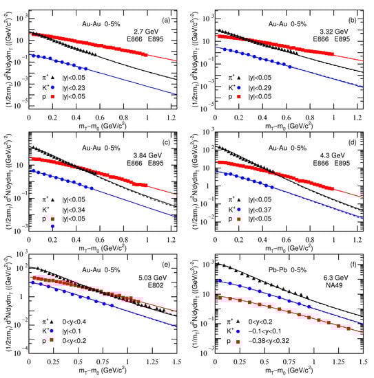
Figure 1.
Transverse mass spectra of charged pions, kaons, and protons produced in 0–5% Au-Au collisions at (a) 2.7, (b) 3.32, (c) 3.84, (d) 4.3, and (e) 5.03 GeV, and in 0–5% Pb-Pb collisions at (f) 6.3 GeV. In panel (f), the factor does not appear, which causes different normalization from other panels. The symbols represent the experimental data at mid-y measured by the E866, E895, and E802 Collaboration at the AGS [31,32,33,34,35] and by the NA49 Collaboration at the SPS [36,37]. The solid and dashed curves are our results, fitted by using Equation (10) due to Equations (7) and (9), with and , respectively.
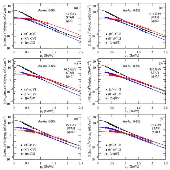
Figure 2.
Transverse momentum spectra of charged pions, kaons, and protons produced in 0–5% Au-Au collisions at (a) 7.7, (b) 11.5, (c) 14.5, (d) 19.6, (e) 27, and (f) 39 GeV. In panel (c), the factor , i.e., the number of events is included on the vertical axis, which can be omitted. The symbols represent the experimental data at mid-y measured by the STAR Collaboration at the RHIC [38,39,40]. The solid and dashed curves are our results, fitted by using Equation (10) due to Equations (7) and (9), with and , respectively.
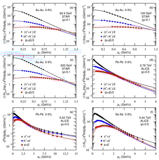
Figure 3.
Transverse momentum spectra of charged pions, kaons, and protons produced in 0–5% Au-Au collisions at (a) 62.4, (b) 130, and (c) 200 GeV; in 0–5% Pb-Pb collisions at (d) 2.76 and (e) 5.02 TeV; and in 0–5% Xe-Xe collisions at (f) 5.44 TeV. In panels (c,d,f), the factor is included on the vertical axis, which can be omitted. In panels (e,f), the item is not included on the vertical axis, which results in different calculation for vertical values from other panels in the normalization. The symbols represent the experimental data at mid-y measured by the STAR Collaboration at the RHIC [38,39,40] and by the ALICE Collaboration at the LHC [41,42,43]. The solid and dashed curves are our results, fitted by using Equation (10) due to Equations (7) and (9), with and , respectively.
Note that the limit of the first and second (low- and high-) components is determined by a convenient treatment. Generally, the contribution fraction k of the first component should be taken as largely as possible. As will be seen in the next section, we take in most cases; only in Figure 3e we take . Because the contribution fraction of the second component is zero or small enough, Equation (10) becomes Equation (9), and the weighted average of the two parameters in Equation (10) becomes the parameter in Equation (9). Because Equations (1), (4), (5), and (7) are suitable at mid-y, Equations (8)–(10) are also suitable at mid-y. In addition, the rapidity ranges quoted in the next section are narrow and around 0, though the concrete ranges are different. This means that the mentioned equations are applicable.
We would like to point out that although the model used by itself is not enough to provide information of the deconfinement phase transition from hadronic matter to QGP, the excitation function of extracted parameter is expected to show some particular tendencies. These particular tendencies include, but are not limited to, the peak and valley structures, the fast and slow variations, the positive and negative changes, etc. These particular tendencies are related to the equation of state (EOS) of the considered matter. The change of EOS reflects the possible change of interaction mechanism from hadron-dominated to parton-dominated intermediate state. Then, the deconfinement phase transition of the considered matter from hadronic matter to QGP is possibly related to the particular tendencies. It is natural that the explanations are not only for a given set of data. The present model will show a method to fit and explain the data.
To obtain , we need to know the slope of versus in the source rest frame of the considered particle. That is, we need to calculate and . According to Equation (10), we have
due to
where denotes the maximum .
As the mean energy, , where p is the momentum of the considered particle in the source rest frame. The analytical calculation of is complex. Instead, we can perform the calculation by the Monte Carlo method. Let denote random numbers distributed evenly in . Each concrete satisfies
where denotes a small shift relative to . Each concrete emission angle satisfies
due to the fact that the particle is assumed to be emitted isotropically in the source rest frame. Each concrete momentum p and energy E can be obtained by
and
respectively.
After repeating calculations multiple times in the Monte Carlo method, we can obtain , that is, . Then, the slope of versus is identified as . Meanwhile, the intercept of T versus is identified as . Here, we emphasize that we have used the alternative method introduced in Section 1 to obtain and .
Note that in some cases, the transverse spectra are shown in terms of , but not . To transform the probability density function of to the probability density function of , we have the relation
Then, we have
due to Equation (2). Using the parameters from spectra, we may also obtain , , , and .
We now discuss the chemical potential of the i-th parton. Generally, the chemical potential of a particle obviously affects the particle production at low energy [52,53,54,55,56,57,58]. For baryons (mostly protons and neutrons), the chemical potential related to collision energy is empirically given by
where both and are in the units of GeV [59,60,61]. According to the authors of [52], we have because a proton or neutron is consists of three quarks (i.e., or ).
3. Results and Discussion
3.1. Comparison with Data and Tendencies of Free Parameters
Figure 1, Figure 2 and Figure 3 present the transverse momentum (transverse mass ) spectra, , of charged pions, kaons, and protons produced in 0–5% Au-Au, Pb-Pb, and Xe-Xe collisions at different . The collision types, particle types, mid-y ranges, centrality classes, and are marked in the panels. The symbols represent the experimental data measured by different collaborations. The solid and dashed curves are our results, fitted by using Equation (10) due to Equations (7) and (9), with and , respectively. In the process of fitting the data, we determine the best parameters by the method of least squares. The experimental uncertainties used in calculating the are obtained by the root sum square of the statistical uncertainties and the systematic uncertainties. The parameters that minimize the are the best parameters. The errors of parameters are obtained by the statistical simulation method [62,63], which uses the same algorithm as usual, if not the same Code, in which the errors are also extracted from variations of . The values of , , k, q, and are listed in Table 1 and Table 2 with the normalization constant (), , and the number of degree of freedom (ndof), or explained in the caption of Table 1.

Table 1.
Values of free parameters (, , q, and ), normalization constant (), , and ndof corresponding to the solid curves in Figure 1, Figure 2 and Figure 3 in which the data are measured in special conditions (mid-y ranges and energies) by different collaborations, where is not available in most cases because . In a few cases (at TeV), is available in the next line, where , which is not listed in the table.
In a few cases, the values of /ndof are very large (5–10 or above), which means “bad” fit to the data. In most cases, the fits are good due to small /ndof which is around 1. To avoid possible wrong interpretation with this result, the number of “bad” fits are limited to be much smaller than that of good fits, for example, 1 to 5 or more strict such as 1 to 10. Meanwhile, we should also use other method to check the quality of fits. In fact, we have also calculated the p-values in the Pearson method. It is shown that all p-values are less than . These p-values corresponds approximately to the Bayes factor being above 100 and to the confidence degree of 99.99994% at around 5 standard deviations () of the statistical significance. This means that the model function is in agreement with the data very well. To say the least, most fits are acceptable.
Note that we will use a set of pion, kaon, and proton spectra to extract and in Section 3.2. For energies in the few GeV range, the spectra of some negative particles are not available in the literature. Therefore, we have to give up to analyze all the negative particle spectra in Figure 1. In our recent work [28], the positive and partial negative particle spectra were analyzed by the standard distribution. The tendencies of parameters are approximately independent of isospin, if not the same for different isospins.
One can see from Figure 1, Figure 2 and Figure 3 and Table 1 and Table 2 that Equation (10) approximately describes the considered experimental data. For all energies and particles, and are identical except for the 5.02 TeV Pb-Pb data from ALICE. This means that none of the spectra have a wide enough range to determine the second component except the data at 5.02 TeV. The two-component fit is only really used at 5.02 TeV. In the high- region, the hard scattering process which is described by the second component in Equation (10) contributes totally. However, in the case of using the two-component function, k () is very close to 1, which implies that the contribution of the second component is negligible. In fact, the second component contributes to the spectrum in high- region with small fraction, which does not affect significantly the extraction of parameters. Instead, the parameters are determined mainly by the spectrum in low- region.
Although the contribution fraction of the second component is very small, the spectra with a wide range on Figure 3e are well fit using the two components, this means increasing the number of parameters compared with just Tsallis function. Generally, the spectrum shapes of different particles are different. However, we may use the same function with different parameters and normalization constants to fit them uniformly. In some cases, the spectrum forms are different. We need to consider corresponding normalization treatments so that the fitting function and the data are compatible and concordant.
The value of affects mainly the parameters at below dozens of GeV. Although is not justified at lower energies, we present the results with for comparison with so that we can have a quantitative understanding on the influence of . Note that is only for and , that is . For pions, we have . For kaons, we have no suitable expression because the chemical potential for s quark is not available here. Generally, . Therefore, .
As a function with wide applications, the Tsallis distribution can describe in fact the spectra presented in Figure 1, Figure 2 and Figure 3 in most cases, though the values of parameters may be changed. However, to extract some information at the parton level, we have regarded the revised Tsallis-like function (Equation (7)) as the components of contributed by the participant partons. The value of is then taken to be the root sum square of the components. In the present work, we have considered two participant partons and two components. This treatment can be extended to three and more participant partons and their components. In the case of the analytical expression for more components becoming difficult, we may use the Monte Carlo method to obtain the components, and is also the root sum square of the components. Then, the distribution of is obtained by the statistical method.
To study the changing trends of the free parameters, Figure 4 shows the dependences of (a) effective temperature T, (b) entropy index q, and (c) revised index on collision energy , where the closed and open symbols are cited from Table 1 and Table 2 which are obtained from the fittings with (solid curves) and (dashed curves) in Figure 1, Figure 2 and Figure 3, respectively. The triangles, circles, squares, and pentagrams represent the results for charged pions, kaons, protons, and the average by weighting different yields, respectively. Because the errors of parameters are very small, the error bars in the plots are invisible. One can see from Figure 4 that T increases significantly, q increases slowly, and increase quickly from to GeV (exactly from 2.7 to 7.7 GeV) and then changes slowly at above 10 GeV, except for a large increase () at the maximum energy, with the increase of . These parameters also show their dependences on particle mass : With the increase of , T and increase and q decreases significantly. Indeed, affects only the parameters at the lower energies (below dozens of GeV), but not higher energy.
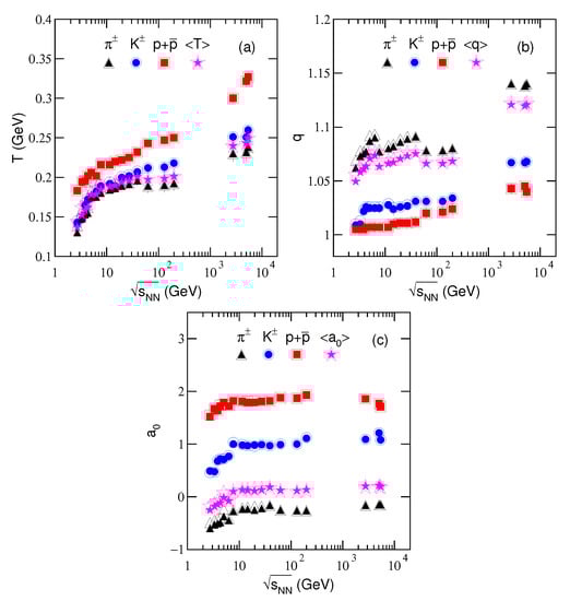
Figure 4.
Dependences of (a) effective temperature T, (b) entropy index q, and (c) revised index on energy , where the closed and open symbols are cited from Table 1 and Table 2 which are obtained from the fittings with (solid curves) and (dashed curves) in Figure 1, Figure 2 and Figure 3, respectively. The triangles, circles, squares, and pentagrams represent the results for charged pions, kaons, protons, and the average by weighting different yields, respectively.
The behavior of excitation function of T will be discussed as that of in the next subsection. The large fluctuations of q for pions are caused by the large influence of strong decay from high-mass resonance and weak decay from heavy flavor hadrons. For light particles such as pions, the influence and then the fluctuations are large; while for relative heavy particles such as kaons and protons, the influence and then the fluctuations are small. No matter how large the fluctuations are, the values of q are close to 1.
As we mentioned in the above section, the entropy index q reflects the degree of equilibrium or non-equilibrium of collision system. Usually, corresponds to an ideal equilibrium state and means a non-equilibrium state. The present work shows that q is very close to 1 which means that the system stays in the equilibrium state. Generally, the equilibrium is relative. For the case of non-equilibrium, we may use the concept of local equilibrium. If q is not too large, for example, or , the collision system is still in equilibrium or local equilibrium [45,64]. In particular, the system is closer to the equilibrium when it emits protons at lower energy, comparing with pions and kaons at higher energy. The reason is that most protons came from the participant nuclei directly. They have enough time to reach to the equilibrium in the evolution. At lower energy, the system is closer to the equilibrium because the evolution is slower and the system has more time to result in the equilibrium. From the initial collisions to kinetic freeze-out, the evolution time is very short. The lower the collision energy is, the longer the evolution time is.
The values of for the spectra of charged pions, kaons, and protons at above 10 GeV are approximately 0.75, 1, and 1.8, respectively, which drop obviously for pions and kaons at lower energy due to the hadronic phase. In addition, due to the existence of participant protons in both the hadronic and QGP phases, the energy dependence of for protons is not obvious. Although it is hard to explain exactly the physical meaning of , we emphasize here that it shows the bending degree of the spectrum in low- region [48,49] and affects the slopes in high- region due to the limitation of normalization. A large bending degree means a large slope change. In fact, is empirically related to the contributions of strong decay from high-mass resonance and weak decay from heavy flavor hadrons. This is because that affects mainly the spectra in low- region which is just the main contribution region of the two decays.
One can see that the values of q and change drastically with particle species. This is an evidence of mass-dependent differential kinetic freeze-out scenario [26]. The massive particles emit earlier than light particles in the system evolution. The earlier emission is caused due to the fact that the massive particles are left behind in the evolution process, but not their quicker thermal and flow motion. In fact, the massive particles have no quicker thermal and flow motion due to larger mass. Instead, light particles have quicker thermal and flow motion and longer evolution time. Finally, light particles reach larger space at the stage of kinetic freeze-out.
The influence of on q and is very small. Although the prefactor can come from the Cooper–Frye term (and/or a kind of saddlepoint integration) as discussed, e.g., in [65,66], it is a fit parameter in this work. As an average over pions, kaons, and protons, is nearly independent of at above 10 GeV. As increasing from ≈3 to ≈10 GeV, the increase of shows different collision mechanisms comparing with that at above 10 GeV. Our recent work [67] shows that the energy ≈10 GeV discussed above is exactly 7.7 GeV.
3.2. Derived Parameters and Their Tendencies
As we know, the effective temperature T contains the contributions of the thermal motions and flow effect [68]. The thermal motion can be described by the kinetic freeze-out temperature , and the flow effect can be described by the transverse flow velocity . To obtain the values of and , we analyze the values of T presented in Table 1 and Table 2, and calculate and based on the values of parameters listed in Table 1 and Table 2. In the calculation performed from to and by the Monte Carlo method, as in [24,25,26], an isotropic assumption in the rest frame of emission source is used.
Figure 5a–f shows the relationship of T and , determined fitting AA collision systems by our model. Figure 6a–f shows the relationship of and , correspondingly. Different symbols represent the values from central AA collisions at different . The symbols in Figure 5a–f represent the values of T for different . The symbols in Figure 6a–f represent the values of for different .
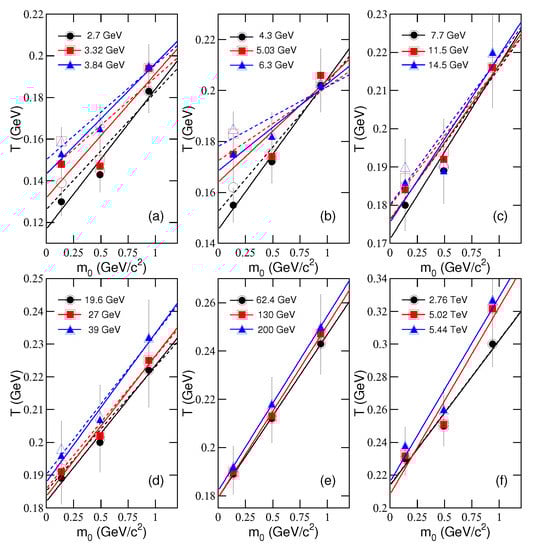
Figure 5.
Dependences of T on . Different symbols represent the results from identified particles produced in central AA collisions at different energies shown in panels (a)–(f). The lines are the results fitted by the least square method, where the intercepts are regarded as . The closed and open symbols (the solid and dashed curves) correspond to the results for and respectively.
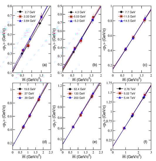
Figure 6.
Different symbols represent the results from identified particles produced in central AA collisions at different energies shown in panels (a)–(f). Same as for Figure 5, but showing the dependences of on . The lines are the results fitted by the least square method, where the slopes are regarded as .
We noted that in Figure 5b, T increases with the energy from 4.3 to 6.3 GeV for the emission of pions and not for protons, while in the case of 2.76–5.44 TeV in Figure 5f, T increases for the emission of protons and not for pions. This discrepancy also appears when narrow energy ranges are fitted in experiments, though should increase for all particle species as a function of . We may explain this as the fluctuations. It is expected that T for emissions of both pions and protons show the same or similar behavior with the energy in a wide range.
It can be seen that the mentioned relationships show nearly linear tendencies in most cases. The lines in Figure 5 and Figure 6 are the results fitted by the least square method, where the solid and dashed lines correspond to the results for and , respectively. The values of intercepts, slopes, and are listed in Table 3 and Table 4. One can see that, in most cases, the mentioned relations are described by a linear function. In particular, the intercepts in Figure 5a–f are regarded as , and the slopes in Figure 6a–f are regarded as , as what we discussed above in the alternative method. Because different “thermometers” are used, extracted from the intercept exceeds (is not in agreement with) the transition temperature which is independently determined by lattice QCD to be around 155 MeV. To compare the two temperatures, we need a transform equation or relation which is not available at present and we will discuss it later.
It is noted that the above argument on and is based usually on exact hydrodynamic calculations, as, e.g., given in [17,65,69,70,71,72]. However, in these cases, usually T is extracted, and then some like correspondence is derived (where instead of , also energy or average energy could stand, depending on the calculation). Here, as we know, is related but not equal to , as discussed in the mentioned literature. Therefore, we give up to use as in this work.
We think that can be also obtained from , and can be also obtained from T. However, the relations between and , as well as and T, are not clear. Generally, the parameters and are model-dependent. In other models, such as the blast-wave model [17,18,19,20,21], and can be obtained conveniently. The two treatments show similar tendencies of parameters on and event centrality, if we also consider the flow effect in small system or peripheral AA collisions [73,74] in the blast-wave model.
In order to more clearly see the tendencies of and , we show the dependences of on , on , and on in Figure 7a–c, respectively. One can see that the two parameters increase quickly from to GeV and then slowly at above 10 GeV with the increase of in general. There is a plateau from near 10 GeV to 200 GeV. In particular, increases with due to the fact that both of them increase with . These incremental tendencies show that, in the stage of kinetic freeze-out, the degrees of excitation and expansion of the system increase with increasing . These results are partly in agreement with the blast-wave model which shows decreasing tendency for and increasing tendency for with increasing from the RHIC [40] to LHC [41] because different partial ranges in the data are considered for different particles, while this work uses the range as wide as the data. The chemical potential shows obvious influence on at the lower energies (below dozens of GeV). After considering the chemical potential, the plateau in the excitation function of becomes more obvious.
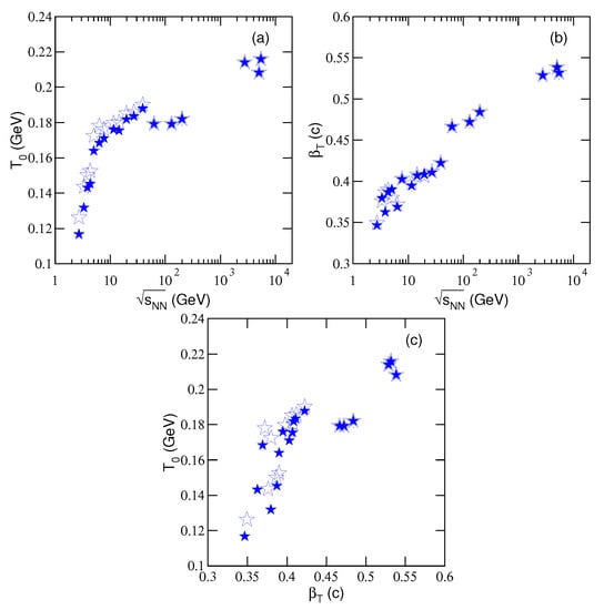
With the increase of , the fact that the values of and increase quickly from to GeV and then slowly at above 10 GeV implies that there are different collision mechanisms in the two energy ranges. In AA collisions, if the baryon-dominated effect plays a more important role at below 10 GeV [75], the meson-dominated effect should play a more important role at above 10 GeV. In the baryon-dominated case, less energies are deposited in the system, and then the system has low excitation degree and temperature. In the meson-dominated case, the situation is opposite. Indeed, GeV is a particular energy which should be paid more attention. It seems that the onset energy of deconfinement phase transition from hadronic matter to QGP is possibly 10 GeV or slightly lower (e.g., 7.7 GeV [67]).
If we regard the plateau from near 10 to 200 GeV in the excitation functions of and as a reflection of the formation of QGP liquid drop, the quick increase of and at the LHC is a reflection of higher temperature QGP liquid drop due to larger energy deposition. At the LHC, the higher collision energy should create larger energy density and blast wave, and then higher and . Although any temperature needs to be bound by the phase transition on one side and free streaming on the other side, larger energy deposition at the LHC may heat the system to a higher temperature even the phase transition temperatures at the LHC and RHIC are the same. Both the formed QGP and hadronized products are also possible to be heated to higher temperature.
Although we mentioned that the plateau apparent in versus is possibly connected to the onset of deconfinement, the temperature measured in this work is connected only to which is usually much smaller than the quark-hadron transition temperature. Because the collision process is very complex, the dependence of reflects only partial properties of the phase structure of a quark medium. To make a determined conclusion, we may connect to the dynamics of the hadron gas. This topic is beyond the focus of the present work and will not be discussed further here.
We would like to point out that, in the last three paragraphs mentioned above, the discussions on the excitation function of presented in Figure 7a are also suitable to the excitation function of T presented in Figure 4a, though the effect of flow is not excluded from Figure 4a. Because the quality of fits is not sufficient in a few cases, our main conclusion that the rise of temperature below 10 GeV suggests that a deconfinement of hadronic matter to QGP is weak. The information of phase transition happened at higher temperatures and near the chemical freeze-out may be reflected at the kinetic freeze-out of a hadronic system. The plateau structure appeared in the excitation function is expected to relate to the phase transition, though this relation is not clear at present. Other works related to this issue are needed to make a strong conclusion. In other words, to conclude the onset of deconfinement just from the quality of some fits is a loose interpretation. More investigations are needed and also comparison with other findings. This issue is beyond the scope of this analysis.
3.3. Further Discussion
The model presented in the analysis can be regarded as a “thermometer” to measure temperatures and other parameters at different energies. Then, the related excitation functions can be obtained, and the differences from the transition around critical point and other energies can be seen. Different models can be regarded as different “thermometers”. The temperatures measured by different “thermometers” have to be unified so that one can give a comparison. If we regard the phase transition temperature determined by lattice QCD as the standard one, the values of obtained in this paper should be revised to fit the standard temperature. However, this revision is not available for us at present due to many uncertain factors. In fact, we try to focus on the “plateau” in the energy dependence of , but not on the values themselves.
In addition, the model assumes the contributions from two participant partons in the framework of multisource thermal model [30]. In pp collisions, one can see the point of a hard scattering between two partons and look at the high particle productions or other observations. However, even in pp collisions there are underlying events, multiple-parton interactions, etc. Further, the data used in this analysis are from central AA collisions, where hundreds and thousands of hadrons are produced. Although many partons take part in the collisions, only a given two-parton process plays main role in the production of a given set of particles. Many two-parton processes exist in the collisions. Using a model inspired by two participant partons is reasonable.
Of course, one may also expect that the production of many particles can result from three or more partons. If necessary, we may extend the picture of two participant partons to that of three or multiple participant partons [30] if we regard of identified particle as the root sum square of the transverse momenta of three or multiple participant partons. It is just that the picture of two participant partons is enough for the production of single particle in this analysis. Besides, we did not try to distinguish between local thermalization of a two-parton process. Instead, we regard the whole system as the same temperature, though which is mass dependent.
The present work is different from the quark coalescence model [66,76,77,78,79,80], though both the models have used the thermalization and statistics. In particular, the quark coalescence model describes classically mesonic prehadrons as quark–anti-quark clusters, and baryonic ones composed from three quarks. The present work describes both mesons and baryons as the products of two participant partons which are regarded as two energy sources.
The assumption of two participant partons discussed in the present work does not mean that the particles considered directly stem from two initial partons of the incoming nuclei. In fact, we assume the two participant partons from the violent collision system in which there is rescattering, recombination, or coalescence. The two participant partons are only regarded as two energy sources to produce a considered particle, whether it is a meson, baryon, or even a lepton [48,49]. The present work treats uniformly the production of final-state particles from the viewpoint of participant energy sources, but not the quark composition of the considered particles [66,76,77,78,79,80].
In the two-component distribution (Equation (10)), the first component contributed by the soft excitation process is from the sea quarks. The second component contributed by the hard scattering process is from the valence quarks. This explanation is different from the Werner’s picture on core–corona separation [81,82,83,84], in which core and corona are simply defined by the density of partons in a particular area of phase or coordinate-space and they distinguish between thermal and non-thermal particle production. This could also be a two-component fit based on the Tsallis function, but its relation to the two-parton dynamics pushed here is not clear. Anyhow, it is possible that the two processes can be described by a uniform method [48,49], though different functions and algorithms are used.
Although there were many papers in the past that have studied the identified particle spectra in high-energy collisions, both experimentally and phenomenologically, this work shows a new way to systemize the experimental data in AA collisions over a wide energy range from 2.7 GeV to 5.44 TeV at the parton level. We emphasize that, in this work, we have analyzed the particle as the root sum square of transverse momenta and of two participant partons. That is, the relation of is used. While, in our recent work [48,49], the relation of is used, which is considered from energy relation at mid-y for massless particle. The scenarios used in this work and our recent work are different. Based on our analyses, it is hard to judge which scenario is more reasonable.
Through the analysis of the data, we have obtained the excitation functions of some quantities, such as T and its weighted average , and its weighted average , and its weighted average , q and its weighted average , as well as and its weighted average . These excitation functions all show some specific laws as increases. Although the conclusion on “onset of deconfinement” or QCD phase transition is indicated around 10 GeV or below is possibly over-interpreting the data and only using the blast-wave or Tsallis-like model is clearly not enough, the sudden change in the slope in the excitation function of is worthy of attention.
4. Summary and Conclusions
We summarize here our main observations and conclusions.
(a) The transverse momentum (mass) spectra of charged pions, kaons, and protons produced at mid-rapidity in central AA (Au-Au, Pb-Pb, and Xe-Xe) collisions over an energy range from 2.7 GeV to 5.44 TeV have been analyzed in this work. The experimental data measured by several collaborations are fitted satisfactorily in the framework of multisource thermal model in which the transverse momentum of identified particle is regarded as the root sum square of transverse momenta of two participant partons, where the latter obeys the revised Tsallis-like function. This treatment for the spectra of transverse momenta is novel and successful. The excitation functions of parameters such as the effective temperature, entropy index, revised index, kinetic freeze-out temperature, and transverse flow velocity are obtained. The chemical potential has obvious influence on the excitation function of kinetic freeze-out temperature at lower energy.
(b) With increasing collision energy, the entropy index increases slowly, and the revised index increases quickly and then changes slowly except for a large increase at the LHC. With increasing the particle mass, the entropy index decreases and the revised index increases obviously. The collision system discussed in this work stays approximately in the equilibrium state, and some functions based on the assumption of equilibrium can be used. The system is closer to the equilibrium state when it emits protons at lower energy, comparing with pions and kaons at higher energy. The revised index describes the bending degrees of the spectra in very low transverse momentum region. Its values for the spectra of charged pions, kaons, and protons are approximately 0.75, 1, and 1.8, respectively, at above 10 GeV and drop obviously at below 10 GeV.
(c) With increasing collision energy, the effective temperature increases clearly and monotonously, and the kinetic freeze-out temperature and transverse flow velocity increase quickly from to GeV and then slowly at above 10 GeV. There is a plateau from near 10 GeV to 200 GeV in the excitation functions of the latter pair. The onset energy of deconfinement phase transition from hadronic matter to QGP is connected to the special changes of excitation function of kinetic freeze-out temperature and possibly 10 GeV or slightly lower. If the plateau at the RHIC is regarded as a reflection of the formation of QGP liquid drop, the following quick increase of the excitation functions at the LHC is a reflection of higher temperature QGP liquid drop due to larger energy deposition. At kinetic freeze-out, the temperature and expansion velocity of the system increase with increasing the energy from the RHIC to LHC.
Author Contributions
L.-L.L., F.-H.L. and K.K.O. contributed equally to this work. All authors have read and agreed to the published version of the manuscript.
Funding
The work of L.-L.L. and F.-H.L. was supported by the National Natural Science Foundation of China under Grant Nos. 12047571, 11575103 and 11947418; the Scientific and Technological Innovation Programs of Higher Education Institutions in Shanxi (STIP) under Grant No. 201802017; the Shanxi Provincial Natural Science Foundation under Grant No. 201901D111043; and the Fund for Shanxi “1331 Project” Key Subjects Construction. The work of K.K.O. was supported by the Ministry of Innovative Development of Uzbekistan within the fundamental project on analysis of open data on heavy-ion collisions at RHIC and LHC.
Institutional Review Board Statement
Not applicable.
Informed Consent Statement
Not applicable.
Data Availability Statement
The data used to support the findings of this study are included within the article and are cited at relevant places within the text as references.
Conflicts of Interest
The authors declare no conflict of interest. The funding agencies have no role in the design of the study; in the collection, analysis, or interpretation of the data; in the writing of the manuscript; or in the decision to publish the results.
References
- Khuntia, A.; Tripathy, S.; Shahoo, R.; Cleymans, J. Multiplicity dependence of non-extensive parameters for strange and multi-strange particles in proton-proton collisions at TeV at the LHC. Eur. Phys. J. A 2017, 53, 103. [Google Scholar] [CrossRef]
- Ahmad, S.; Ahmad, A.; Chandra, A.; Zafar, M.; Irfan, M. Entropy analysis in relativistic heavy-ion collisions. Adv. High Energy Phys. 2013, 2013, 836071. [Google Scholar] [CrossRef]
- Bjorken, J.D. Highly relativistic nucleus-nucleus collisions: The central rapidity region. Phys. Rev. D 1983, 27, 140–151. [Google Scholar] [CrossRef]
- Dusling, K. From initial-state fluctuations to final-state observables. Nucl. Phys. A 2013, 904–905, 59c–66c. [Google Scholar] [CrossRef]
- Gyulassy, M.; Mclerran, L. New forms of QCD matter discovered at RHIC. Nucl. Phys. A 2005, 750, 30–63. [Google Scholar] [CrossRef]
- Tawfik, A.N. Equilibrium statistical-thermal models in high-energy physics. Int. J. Mod. Phys. A 2014, 29, 1430021. [Google Scholar] [CrossRef]
- Gupta, S.; Luo, X.F.; Mohanty, B.; Ritter, H.G.; Xu, N. Scale for the phase diagram of quantum chromodynamics. Science 2011, 332, 1525–1528. [Google Scholar] [CrossRef]
- Xu, N. for the STAR Collaboration. An overview of STAR experimental results. Nucl. Phys. A 2014, 931, 1–12. [Google Scholar] [CrossRef]
- Andronic, A.; Braun-Munzinger, P.; Redlich, K.; Stachel, J. Decoding the phase structure of QCD via particle production at high energy. Nature 2018, 561, 321–330. [Google Scholar] [CrossRef]
- Luo, X.F.; Xu, N. Search for the QCD critical point with fluctuations of conserved quantities in relativistic heavy-ion collisions at RHIC: An overview. Nucl. Sci. Tech 2017, 28, 112. [Google Scholar] [CrossRef]
- Tawfik, A.N.; Yassin, H.; Abo Elyazeed, E.R. Extensive/nonextensive statistics for pT distributions of various charged particles produced in p+p and A+A collisions in a wide range of energies. arXiv 2019, arXiv:1905.12756. [Google Scholar]
- Tawfik, A.N. Analogy of QCD hadronization and Hawking-Unruh radiation at NICA. Eur. Phys. J. A 2016, 52, 254. [Google Scholar] [CrossRef]
- Tawfik, A.N.; Yassin, H.; Abo Elyazeed, E.R. Chemical freezeout parameters within generic nonextensive statistics. Indian J. Phys. 2018, 92, 1325–1335. [Google Scholar] [CrossRef]
- Bhattacharyya, S.; Biswas, D.; Ghosh, S.K.; Ray, R.; Singha, P. Novel scheme for parametrizing the chemical freeze-out surface in heavy ion collision experiments. Phys. Rev. D 2019, 100, 054037. [Google Scholar] [CrossRef]
- Bhattacharyya, S.; Biswas, D.; Ghosh, S.K.; Ray, R.; Singha, P. Systematics of chemical freeze-out parameters in heavy-ion collision experiments. Phys. Rev. D 2020, 101, 054002. [Google Scholar] [CrossRef]
- Biswas, D. Centrality dependence of chemical freeze-out parameters and strangeness equilibration in RHIC and LHC. arXiv 2020, arXiv:2003.10425. [Google Scholar]
- Schnedermann, E.; Sollfrank, J.; Heinz, U. Thermal phenomenology of hadrons from 200A GeV S+S collisions. Phys. Rev. C 1993, 48, 2462–2475. [Google Scholar] [CrossRef]
- Abelev, B.I.; Aggarwal, M.M.; Ahammed, Z.; Alakhverdyants, A.V.; Anderson, B.D.; Arkhipkin, D.; Averichev, G.S.; Balewski, J.; Barannikova, O.; Barnby, L.S.; et al. Identified particle production, azimuthal anisotropy, and interferometry measurements in Au+Au collisions at = 9.2 GeV. Phys. Rev. C 2010, 81, 024911. [Google Scholar] [CrossRef]
- Tang, Z.B.; Xu, Y.C.; Ruan, L.J.; Van Buren, G.; Wang, F.Q.; Xu, Z.B. Spectra and radial flow in relativistic heavy ion collisions with Tsallis statistics in a blast-wave description. Phys. Rev. C 2009, 79, 051901(R). [Google Scholar] [CrossRef]
- Tang, Z.B.; Yi, L.; Ruan, L.J.; Shao, M.; Chen, H.F.; Li, C.; Mohanty, B.; Sorensen, P.; Tang, A.H.; Xu, Z.B. Statistical origin of constituent-quark scaling in the QGP hadronization. Chin. Phys. Lett. 2013, 30, 031201. [Google Scholar] [CrossRef]
- Jiang, K.; Zhu, Y.Y.; Liu, W.T.; Chen, H.F.; Li, C.; Ruan, L.J.; Tang, Z.B.; Xu, Z.B. Onset of radial flow in p+p collisions. Chin. Phys. Lett. 2015, 91, 024910. [Google Scholar]
- Heiselberg, H.; Levy, A.M. Elliptic flow and Hanbury-Brown-Twiss correlations in noncentral nuclear collisions. Phys. Rev. C 1999, 59, 2716–2727. [Google Scholar] [CrossRef]
- Takeuchi, S.; Murase, K.; Hirano, T.; Huovinen, P.; Nara, Y. Effects of hadronic rescattering on multistrange hadrons in high-energy nuclear collisions. Phys. Rev. C 2015, 92, 044907. [Google Scholar] [CrossRef]
- Wei, H.-R.; Liu, F.-H.; Lacey, R.A. Kinetic freeze-out temperature and flow velocity extracted from transverse momentum spectra of final-state light flavor particles produced in collisions at RHIC and LHC. Eur. Phys. J. A 2016, 52, 102. [Google Scholar] [CrossRef]
- Wei, H.-R.; Liu, F.-H.; Lacey, R.A. Disentangling random thermal motion of particles and collective expansion of source from transverse momentum spectra in high energy collisions. J. Phys. G 2016, 43, 125102. [Google Scholar] [CrossRef]
- Lao, H.-L.; Wei, H.-R.; Liu, F.-H.; Lacey, R.A. An evidence of mass-dependent differential kinetic freeze-out scenario observed in Pb-Pb collisions at 2.76 TeV. Eur. Phys. J. A 2016, 52, 203. [Google Scholar] [CrossRef]
- Li, L.-L.; Liu, F.-H. Energy dependent kinetic freeze-out temperature and transverse flow velocity in high energy collisions. Eur. Phys. J. A 2018, 54, 169. [Google Scholar] [CrossRef]
- Li, L.-L.; Liu, F.-H.; Waqas, M.; Al-Yusufi, R.; Mujear, A. Excitation functions of related parameters from transverse momentum (mass) spectra in high energy collisions. Adv. High Energy Phys. 2020, 2020, 5356705. [Google Scholar] [CrossRef]
- Zheng, H.; Zhu, L.L. Comparing the Tsallis distribution with and without thermodynamical description in p+p collisions. Adv. High Energy Phys. 2016, 2016, 9632126. [Google Scholar] [CrossRef]
- Liu, F.-H.; Gao, Y.-Q.; Tian, T.; Li, B.-C. Unified description of transverse momentum spectrums contributed by soft and hard processes in high-energy nuclear collisions. Eur. Phys. J. A 2014, 50, 94. [Google Scholar] [CrossRef]
- Ahle, L.; Akiba, Y.; Ashktorab, K.; Baker, M.D.; Beavis, D.; Budick, B.; Chang, J.; Chasman, C.; Chen, Z.; Chu, Y.Y.; et al. Excitation function of K+ and π+ production in Au+Au reactions at 2–10A GeV. Phys. Lett. B 2000, 476, 1–8. [Google Scholar] [CrossRef]
- Klay, J.L.; Ajitanand, N.N.; Alexander, J.M.; Anderson, M.G.; Best, D.; Brady, F.P.; Case, T.; Caskey, W.; Cebra, D.; Chance, J.L.; et al. Longitudinal flow from (2–8)A GeV central Au+Au collisions. Phys. Rev. Lett. 2002, 88, 102301. [Google Scholar] [CrossRef] [PubMed]
- Klay, J.L.; Ajitanand, N.N.; Alexander, J.M.; Anderson, M.G.; Best, D.; Brady, F.P.; Case, T.; Caskey, W.; Cebra, D.; Chance, J.L.; et al. Charged pion production in 2A to 8A GeV central Au+Au Collisions. Phys. Rev. C 2003, 68, 054905. [Google Scholar] [CrossRef]
- Ahle, L.; Akiba, Y.; Ashktorab, K.; Baker, M.D.; Beavis, D.; Britt, H.C.; Chang, J.; Chasman, C.; Chen, Z.; Chi, C.Y.; et al. Kaon production in Au+Au collisions at 11.6 A GeV/c. Phys. Rev. C 1998, 58, 3523–3538. [Google Scholar] [CrossRef]
- Ahle, L.; Akiba, Y.; Ashktorab, K.; Baker, M.D.; Beavis, D.; Britt, H.C.; Chang, J.; Chasman, C.; Chen, Z.; Chi, C.Y.; et al. Particle production at high baryon density in central Au+Au reactions at 11.6A GeV/c. Phys. Rev. C 1998, 57, R466–R470. [Google Scholar] [CrossRef]
- Alt, C.; Anticic, T.; Baatar, B.; Barna, D.; Bartke, J.; Betev, L.; Białkowska, H.; Blume, C.; Boimska, B.; Botje, M.; et al. Pion and kaon production in central Pb+Pb collisions at 20A and 30A GeV: Evidence for the onset of deconfinement. Phys. Rev. C 2008, 77, 024903. [Google Scholar] [CrossRef]
- Afanasiev, S.V.; Anticic, T.; Barna, D.; Bartke, J.; Barton, R.A.; Behler, M.; Betev, L.; Białkowska, H.; Billmeier, A.; Blume, C.; et al. Energy dependence of pion and kaon production in central Pb+Pb collisions. Phys. Rev. C 2002, 66, 054902. [Google Scholar] [CrossRef]
- Adamczyk, L.; Adkins, J.K.; Agakishiev, G.; Aggarwal, M.M.; Ahammed, Z.; Ajitanand, N.N.; Alekseev, I.; Anderson, D.M.; Aoyama, R.; Aparin, A.; et al. Bulk properties of the medium produced in relativistic heavy-ion collisions from the beam energy scan program. Phys. Rev. C 2017, 96, 044904. [Google Scholar] [CrossRef]
- Bairathi, V. For the STAR Collaboration. Study of the bulk properties of the system formed in Au+Au collisions at = 14.5 GeV using the STAR detector at RHIC. Nucl. Phys. A 2016, 956, 292–295. [Google Scholar] [CrossRef]
- Abelev, B.I.; Aggarwal, M.M.; Ahammed, Z.; Anderson, B.D.; Arkhipkin, D.; Averichev, G.S.; Bai, Y.; Balewski, J.; Barannikova, O.; Barnby, L.S.; et al. Systematic measurements of identified particle spectra in pp, d+Au, and Au+Au collisions at the STAR detector. Phys. Rev. C 2009, 79, 034909. [Google Scholar] [CrossRef]
- Abelev, B.; Adam, J.; Adamová, D.; Adare, A.M.; Aggarwal, M.M.; Rinella, G.A.; Agnello, M.; Agocs, A.G.; Agostinelli, A.; Ahammed, Z.; et al. Centrality dependence of π, K, and p production in Pb-Pb collisions at = 2.76 TeV. Phys. Rev. C 2013, 88, 044910. [Google Scholar] [CrossRef]
- Vázquez, O. New results on collectivity with ALICE. Proceedings for a Parallel Session Talk at the Fifth Annual Large Hadron Collider Physics Conference, May 15–20, 2017. arXiv 2017, arXiv:1710.04715. [Google Scholar]
- Ragoni, S. Production of pions, kaons and protons in Xe-Xe collisions at = 5.44 TeV. PoS 2018, LHCP2018, 085. [Google Scholar]
- Tsallis, C. Possible generalization of Boltzmann-Gibbs statistics. J. Stat. Phys. 1988, 52, 479–487. [Google Scholar] [CrossRef]
- Biró, T.S.; Purcsel, G.; Ürmössy, K. Non-extensive approach to quark matter. Eur. Phys. J. A 2009, 40, 325–340. [Google Scholar] [CrossRef]
- Cleymans, J.; Worku, D. Relativistic thermodynamics: Transverse momentum distributions in high-energy physics. Eur. Phys. J. A 2012, 48, 160. [Google Scholar] [CrossRef]
- Cleymans, J.; Paradza, M.W. Tsallis statistics in high energy physics: Chemical and thermal freeze-outs. Physics 2020, 2, 654–664. [Google Scholar] [CrossRef]
- Yang, P.-P.; Liu, F.-H.; Sahoo, R. A new description of transverse momentum spectra of identified particles produced in proton-proton collisions at high energies. Adv. High Energy Phys. 2020, 2020, 6742578. [Google Scholar] [CrossRef]
- Yang, P.-P.; Duan, M.-Y.; Liu, F.-H. Dependence of related parameters on centrality and mass in a new treatment for transverse momentum spectra in high energy collisions. Eur. Phys. J. A 2021, 57, 63. [Google Scholar] [CrossRef]
- Yang, P.-P.; Wang, Q.; Liu, F.-H. Mutual derivation between arbitrary distribution forms of momenta and momentum components. Int. J. Theor. Phys. 2019, 58, 2603–2618. [Google Scholar] [CrossRef]
- Zhou, G.-R. Probability Theory and Mathamatic and Physics Statsitics; Higher Education Press: Beijing, China, 1984. [Google Scholar]
- Braun-Munzinger, P.; Wambach, J. Colloquium: Phase diagram of strongly interacting matter. Rev. Mod. Phys. 2009, 81, 1031–1050. [Google Scholar] [CrossRef]
- Cleymans, J.; Oeschler, H.; Redlich, K.; Wheaton, S. Comparison of chemical freeze-out criteria in heavy-ion collisions. Phys. Rev. C 2006, 73, 034905. [Google Scholar] [CrossRef]
- Andronic, A.; Braun-Munzinger, P. Ultrarelativistic nucleus-nucleus collisions and the quark-gluon plasma. In Proceedings of the 8th Hispalensis International Summer School on Exotic Nuclear Physics: The Hispalensis Lectures on Nuclear Physics, Seville, Spain, 9–21 June 2003; Volume 2, pp. 35–67. [Google Scholar]
- Rozynek, J.; Wilk, G. Nonextensive effects in the Nambu-Jona-Lasinio model of QCD. J. Phys. G 2009, 36, 125108. [Google Scholar] [CrossRef]
- Rozynek, J.; Wilk, G. Nonextensive Nambu-Jona-Lasinio model of QCD matter. Eur. Phys. J. A 2016, 52, 13. [Google Scholar] [CrossRef]
- Shen, K.M.; Zhang, H.; Hou, D.F.; Zhang, B.W.; Wang, E.K. Chiral phase transition in linear sigma model with nonextensive statistical mechanics. Adv. High Energy Phys. 2017, 2017, 4135329. [Google Scholar] [CrossRef]
- Zhao, Y.P. Th8ermodynamic properties and transport coefficients of QCD matter within the nonextensive Polyako-Nambu-Jona-Lasinio model. Phys. Rev. D 2020, 101, 096006. [Google Scholar] [CrossRef]
- Andronic, A.; Braun-Munzinger, P.; Stachel, J. Thermal hadron production in relativistic nuclear collisions. Acta Phys. Pol. B 2009, 40, 1005–1012. [Google Scholar]
- Andronic, A.; Braun-Munzinger, P.; Stachel, J. The horn, the hadron mass spectrum and the QCD phase diagram: The statistical model of hadron production in central nucleus-nucleus collisions. Nucl. Phys. A 2010, 834, 237c–240c. [Google Scholar] [CrossRef]
- Andronic, A.; Braun-Munzinger, P.; Stachel, J. Hadron production in central nucleus-nucleus collisions at chemical freeze-out. Nucl. Phys. A 2006, 772, 167–199. [Google Scholar] [CrossRef]
- Zhang, H.-X.; Shan, P.-J. Statistical simulation method for determinating the errors of fit parameters. In Proceedings of the 8th National Conferences on Nuclear Physiscs (Volume II), Xi’an, China, 3–7 December 1991; (In Chinese). Available online: http://cpfd.cnki.com.cn/Article/CPFDTOTAL-HWLX199112002128.htm (accessed on 1 March 2021).
- Avdyushev, V.A. A new method for the statistical simulation of the virtual values of parameters in inverse orbital dynamics problems. Sol. Syst. Res. 2009, 43, 543–551. [Google Scholar] [CrossRef]
- Biró, T.S.; Ürmössy, K. Pions and kaons from stringy quark matter. J. Phys. G 2009, 36, 064044. [Google Scholar] [CrossRef]
- Csanád, M.; Vargyas, M. Observables from a solution of (1+3)-dimensional relativistic hydrodynamics. Eur. Phys. J. A 2010, 44, 473–478. [Google Scholar] [CrossRef]
- Ürmössy, K.; Biró, T.S. Cooper-Frye formula and non-extensive coalescence at RHIC energy. Phys. Lett. B 2010, 689, 14–17. [Google Scholar] [CrossRef]
- Waqas, M.; Liu, F.-H.; Wang, R.-Q.; Siddique, I. Energy scan/dependence of kinetic freeze-out scenarios of multi-strange and other identified particles in central nucleus-nucleus collisions. Eur. Phys. J. A 2020, 56, 188. [Google Scholar] [CrossRef]
- Li, L.-L.; Liu, F.-H. Kinetic freeze-out properties from transverse momentum spectra of pions in high energy proton-proton collisions. Physics 2020, 2, 277–308. [Google Scholar] [CrossRef]
- Adler, S.S.; Afanasiev, S.; Aidala, C.; Ajitan, N.N.; Akiba, Y.; Alexander, J.; Amirikas, R.; Aphecetche, L.; Aronson, S.H.; Averbeck, R.; et al. Identified charged particle spectra and yields in Au+Au collisions at = 200 GeV. Phys. Rev. C 2004, 69, 034909. [Google Scholar] [CrossRef]
- Csörgo, T.; Lörstad, B. Bose-Einstein correlations for three-dimensionally expanding, cylindrically symmetric, finite systems. Phys. Rev. C 1996, 54, 1390–1403. [Google Scholar] [CrossRef]
- Csörgo, T.; Akkelin, S.V.; Hama, Y.; Lukács, B.; Sinyukov, Y.M. Observables and initial conditions for selfsimilar ellipsoidal flows. Phys. Rev. C 2003, 67, 034904. [Google Scholar] [CrossRef]
- Csanád, M.; Csörgo, T.; Lörstad, B. Buda-Lund hydro model for ellipsoidally symmetric fireballs and the elliptic flow at RHIC. Nucl. Phys. A 2004, 742, 80–94. [Google Scholar] [CrossRef]
- Lao, H.-L.; Liu, F.-H.; Li, B.-C.; Duan, M.-Y. Kinetic freeze-out temperatures in central and peripheral collisions: Which one is larger? Nucl. Sci. Tech. 2018, 29, 82. [Google Scholar] [CrossRef]
- Lao, H.-L.; Liu, F.-H.; Li, B.-C.; Duan, M.-Y.; Lacey, R.A. Examining the model dependence of the determination of kinetic freeze-out temperature and transverse flow velocity in small collision system. Nucl. Sci. Tech. 2018, 29, 164. [Google Scholar] [CrossRef]
- Cleymans, J. The physics case for the ≈ 10 GeV energy region. in Walter Greiner Memorial Volume, edited by P. O. Hess (World Scientiflc, Singapore) (2018). arXiv 2017, arXiv:1711.02882. [Google Scholar]
- Biró, T.S.; Zimányi, J. Quarkochemistry in relativistic heavy ion collisions. Phys. Lett. B 1982, 113, 6–10. [Google Scholar] [CrossRef]
- Biró, T.S.; Zimányi, J. Quark-gluon plasma formation in heavy ion collisions and quarkochemistry. Nucl. Phys. A 1983, 395, 525–538. [Google Scholar] [CrossRef]
- Biró, T.S.; Lévai, P.; Zimányi, J. ALCOR: A dynamic model for hadronization. Phys. Lett. B 1995, 347, 6–12. [Google Scholar] [CrossRef]
- Zimányi, J.; Biró, T.S.; Csörgö, T.; Lévai, P. Particle spectra from the ALCOR model. Heavy Ion Phys. 1996, 4, 15–32. [Google Scholar]
- Biró, T.S.; Lévai, P.; Zimányi, J. Quark coalescence in the mid-rapidity region at RHIC. J. Phys. G 2002, 28, 1561–1566. [Google Scholar]
- Werner, K. Core-corona separation in ultra-relativistic heavy ion collisions. Phys. Rev. Lett. 2007, 98, 152301. [Google Scholar] [CrossRef] [PubMed]
- Aichelin, J.; Werner, K. Core-corona model describes the centrality dependence of v2/ϵ. J. Phys. G 2010, 37, 94006. [Google Scholar] [CrossRef]
- Schreiber, C.; Werner, K.; Aichelin, J. Identified particle spectra for Au+Au collisions at = 200 GeV from STAR, PHENIX and BRAHMS in comparison to core-corona model predictions. Proceedings to the Workshop on Dense Matter—DM 2010, Stellenbosch, South Africa, April 2010. arXiv 2010, arXiv:1012.2066. [Google Scholar]
- Petrovici, M.; Berceanu, I.; Pop, A.; Târzilaˇ, M.; Andrei, C. Core-corona interplay in Pb-Pb collisions at = 2.76 TeV. Phys. Rev. C 2017, 96, 014908. [Google Scholar] [CrossRef]


Publisher’s Note: MDPI stays neutral with regard to jurisdictional claims in published maps and institutional affiliations. |
© 2021 by the authors. Licensee MDPI, Basel, Switzerland. This article is an open access article distributed under the terms and conditions of the Creative Commons Attribution (CC BY) license (https://creativecommons.org/licenses/by/4.0/).