1. Introduction
In 1970, the economist Eugene F. Fama put forward the efficient market hypothesis (EMH), which became the cornerstone of contemporary financial theory. In this hypothesis, all information on the market will be quickly reflected in the stock price, so the stock prices are unpredictable [
1]. However, later behavioral finance theory studies of market behavior have shown the limitations of the EMH. The criticisms focus on the irrationality of investors, market friction and incomplete arbitrage, which are in violation of the effective market hypothesis [
2,
3,
4]. In empirical terms, momentum effects, reversal effects, January effects, and financial anomalies such as peaks and thick tails of time series, volatility clustering, etc. were also found in financial time series [
5,
6,
7,
8,
9]. Hence, economists have actively sought new theories to explain these market anomalies. In 1994, Peters proposed the fractal market hypothesis (FMH). This hypothesis modifies the strict assumptions of the efficient market, pointing out that asset prices obey fractional Brownian motion, the return rate sequence has long memory, and the market may be in a non-equilibrium state [
10]. Therefore, a certain level of predictability of prices has become a general consensus. After the FMH was proposed, the field mainly focused on two aspects, the study of the fractal characteristics of the stock market and building various models to try to predict market trends.
For the first aspect, regarding the method of studying fractal properties, the starting point is the rescaled range method (R/S) proposed by the British hydrologist Hurst [
11]. When studying the relationship between the Nile Reservoir discharge and the water level, he found that a biased random walk (fractional Brownian motion) can well describe the long-term dependence of the two, so he proposed calculating the Hurst exponent by the rescaled range method, which was used for characterizing the self-similarity of time series. Many scholars have continuously optimized and improved the method. Peng et al., proposed the detrending fluctuation analysis method (DFA) when studying the long-range power-law correlation characteristics of DNA sequences, which became the mainstream for measuring the long-range correlation of stationary time series [
12]. However, Kantelhardt et al., pointed out that in most cases, the scaling behavior of time series is very complicated and cannot be explained by a simple scaling index [
13]. Therefore, the multifractal detrending volatility method (MF-DFA) was proposed and the author pointed out that a multifractal structure may come from the thick-tailed distribution and long-range correlation. Thompson et al., used multi-methods for analyzing the fractal characteristics of GE stock price series. The results showed that the MF-DFA model is better fitted [
14]. A number of existing studies have shown that multifractals are common in financial markets in various countries, including stock markets [
15,
16,
17,
18,
19], bonds [
20] and Bitcoin markets [
21]. The results above definitely all rejected the efficient market hypothesis. However, some scholars questioned the MF-DFA method. After comparing DFA, CMA, MF-DFA and other detrend volatility analysis methods, Bashan pointed out that the MF-DFA may result in false fluctuations, which may be reflected in the larger calculated generalized Hurst index [
22]. This happens because the intervals divided by the MF-DFA method do not overlap, so the fitting polynomials of adjacent intervals may be discontinuous. Recognizing this shortcoming, many scholars use overlapping smoothing windows to optimize the model respectively, which reduces the spurious fluctuations caused by partially overlapping adjacent intervals [
23,
24]. We adopt this optimization method, which is called OSW-MF-DFA. Some scholars have studied the multifractal changes of the financial market under the impact of the pandemic and confirmed the reduction of market efficiency caused by COVID-19 [
25,
26,
27]. Okorie studied the contagion effect of the fractal of the stock market, which proved the existence of multifractals from another aspect [
28].
For the second aspect of predicting market trends, although stock markets are affected by various factors such as macroeconomic development, institutions, supervision, noise trading etc., researchers still try to construct various prediction models: from parametric models such as ARMA, ARIMA, and GARCH to machine learning such as BP, recurrent neural network (RNN), LSTM and GRU with gated structure, the prediction accuracy of the model has been continuously improved. The short-term memory neural network (LSTM) was proposed by Hochreiter and Schmidhuber in 1997 [
29]. The gated recurrent networks LSTM and GRU, which have been popular in recent years, have been widely used to predict the trend of stock prices, and they have actually proved to have achieved good results by catching the long and short term memory of financial time series [
30,
31,
32]. Yu et al., used the GARCH model and LSTM neural network to predict the volatility of China’s three major stock indexes, and the results proved that LSTM with long memory has better predictive ability [
33]. However, with the popularization of LSTM, more and more studies have found that LSTM models have flaws such as limited explanatory power and slow convergence speed. Aiming at the shortcomings of LSTM, Cho et al., further optimized on the basis of LSTM and proposed a GRU neural network [
34]. Compared with LSTM, GRU has only two gate control structures: update gate and reset gate, which reduces parameters while maintaining predictive performance, and it helps to speed up convergence [
35,
36].
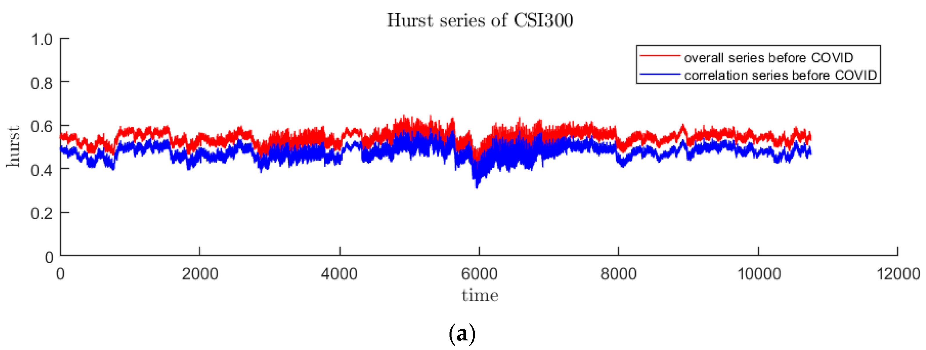
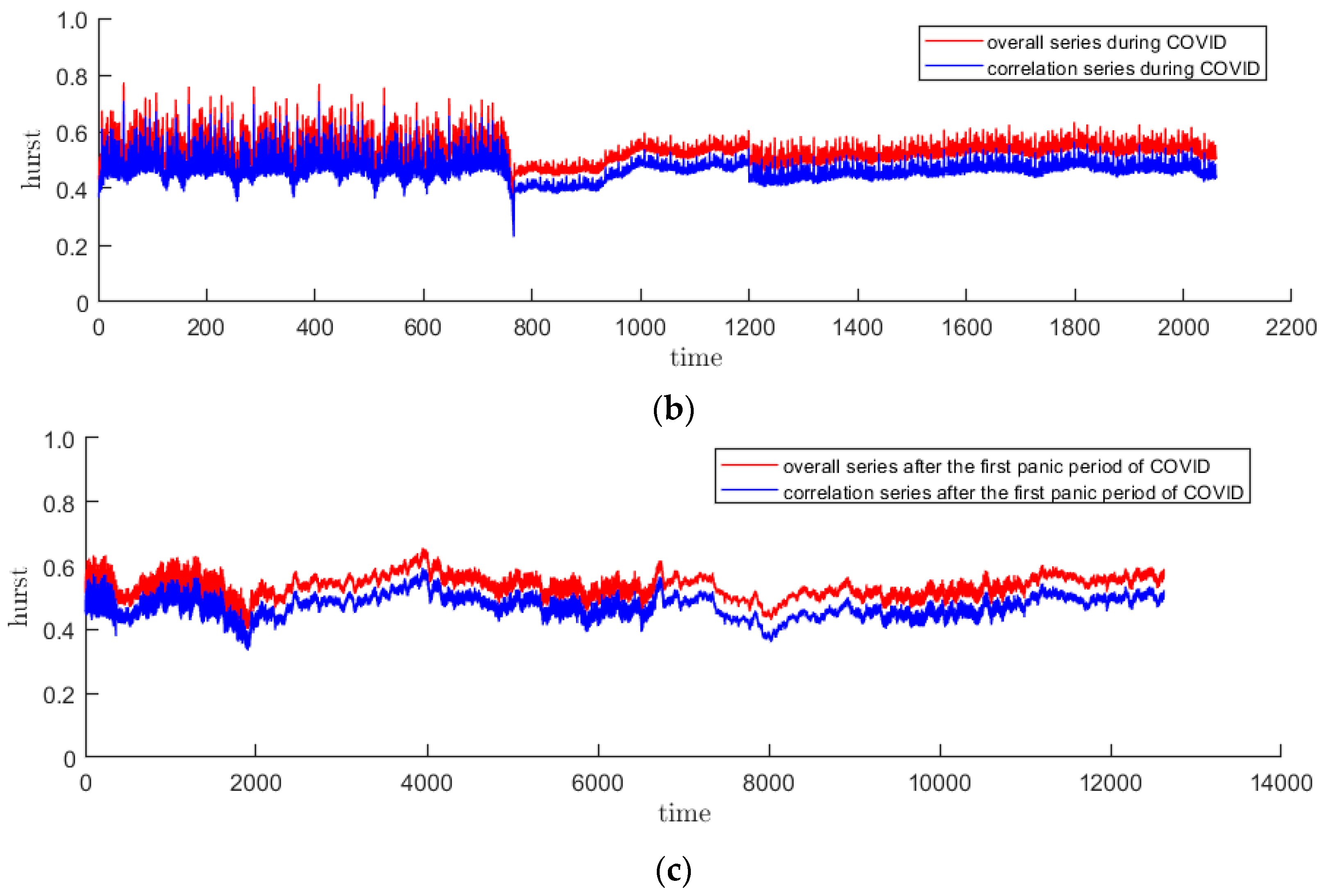
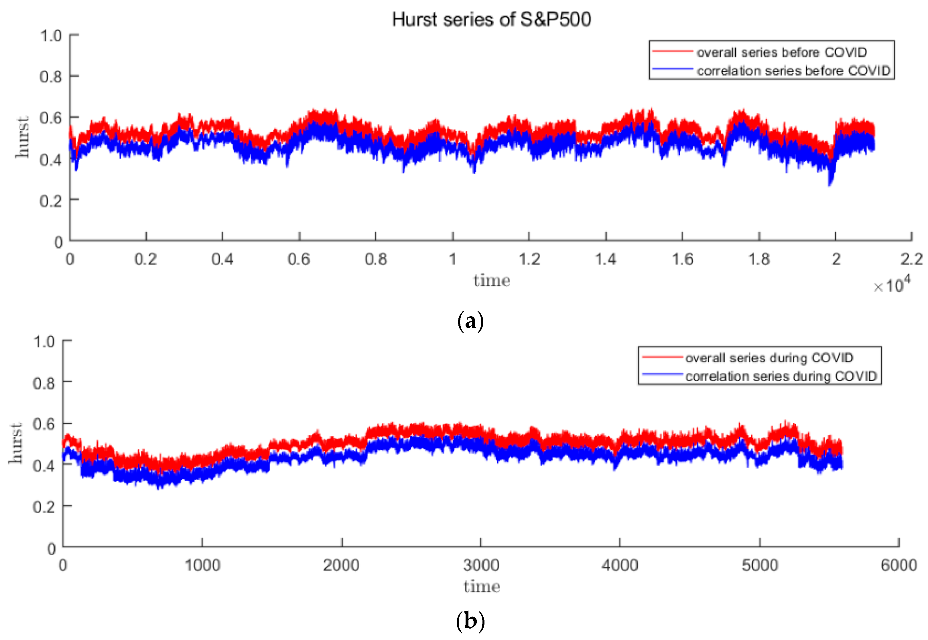
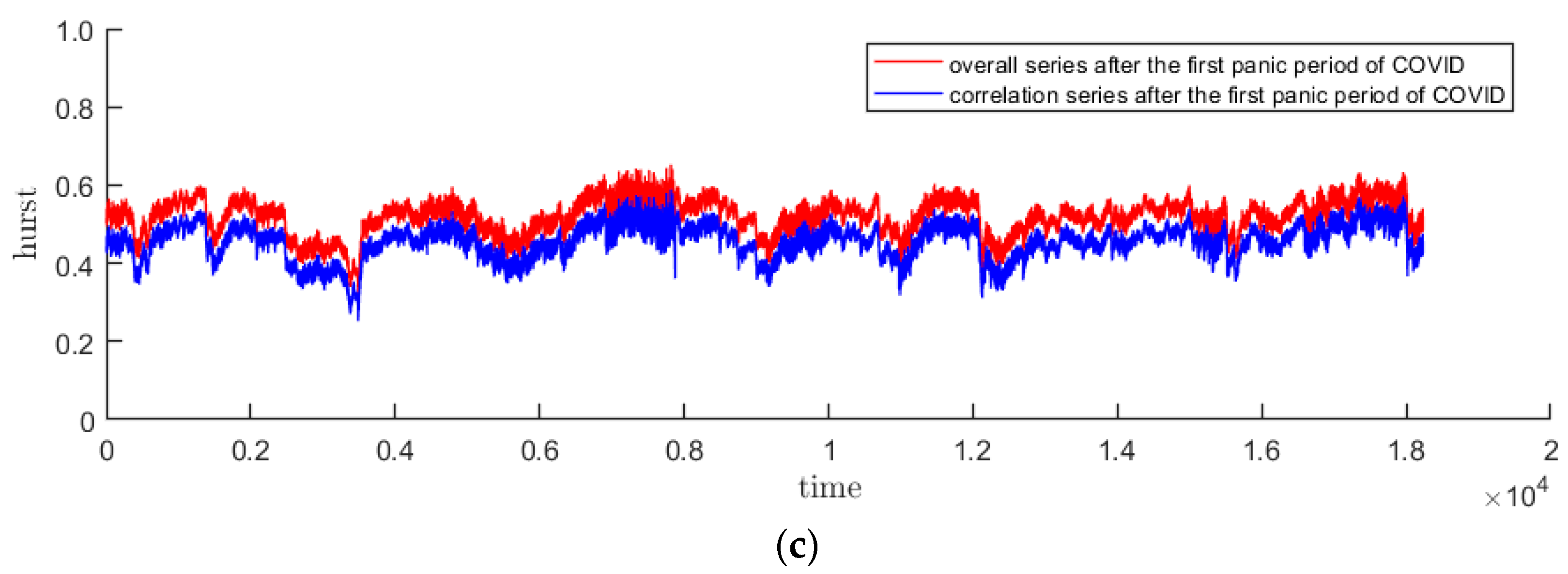
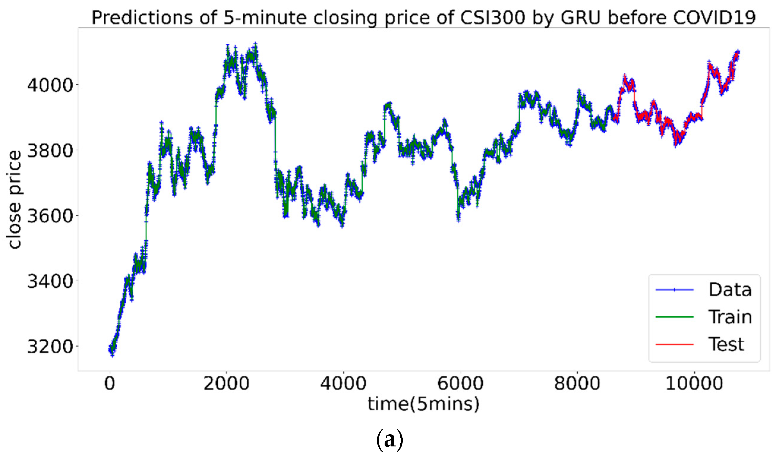
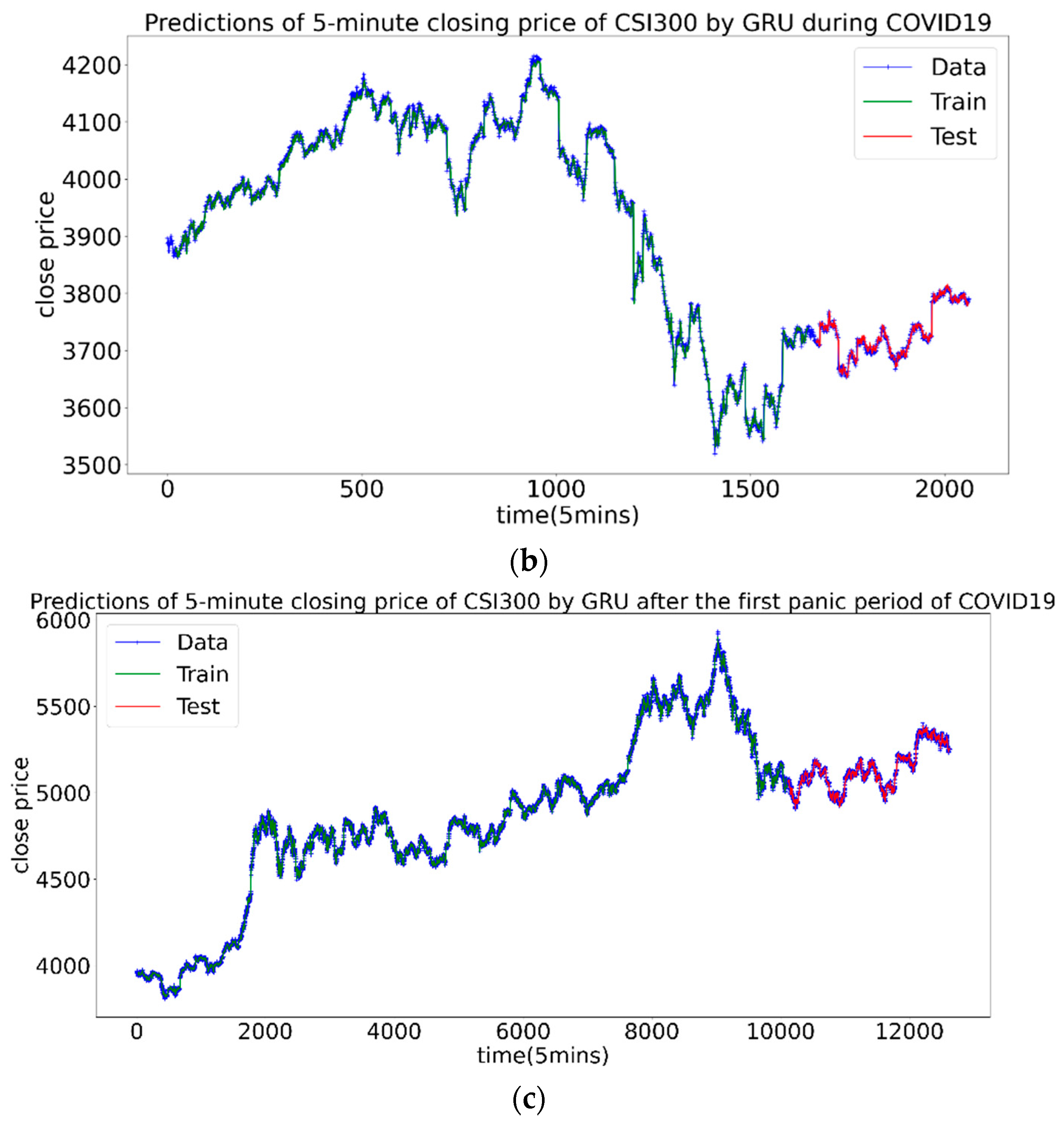
In this article we aim to study the fractal properties of the Chinese and American intraday stock markets under the impact of the COVID-19 pandemic and use them to forecast by applying to the GRU model. According to the impact of the pandemic on the financial markets, we divide the time interval into three periods: before, during and after the first panic period of pandemic. In terms of multifractal research, this article utilizes the OSW-MF-DFA method optimized by overlapping smoothing windows. We obtain the generalized Hurst index and multifractal spectrum of the two stock indexes, then analyze and compare the fractal characteristics of the two markets at different periods. The time-varying Hurst exponent and its decomposition sequence are calculated by the DFA method, which are used as the input variables of the subsequent predictions. A time-varying Hurst sequence is also added to regular input variables such as opening price, closing price, highest price, lowest price, and volatility in GRU neural network, to explore whether it can improve forecasting efficiency.
Through empirical tests, we found that the two markets always have multifractal characteristics, and the degree of fractal intensifies during the pandemic. Among them, the US market was more affected by the pandemic. When putting time-varying Hurst and its decomposition sequence into the prediction model as inputs, we found that they can significantly improve the prediction performance of the model and outperform the volatility indicators during the panic period of pandemics (COVID-19) which has high volatility clustering.
2. Materials and Methods
2.1. Data
This article uses the CSI300 Index and the S&P 500 Index as representatives of the Chinese and US stock markets. The research sample is 5-min intraday data from 1 January 2019 to 9 June 2021. The CSI300 Index is China’s first cross-market index that reflects the overall Shanghai and Shenzhen markets. It consists of 300 mainstream stocks with the best market capitalization and liquidity in the Chinese stock market. It is the investment benchmark most valued by investors. Covering 500 high-quality companies on major exchanges such as the New York Stock Exchange and the Nasdaq, the S&P500 Index was established by the world’s authoritative rating agency Standard & Poor’s. It can reflect the entire picture of the US stock market. The initial indicators are the 5-min opening price, closing price, lowest price, and highest price. The data comes from the Wind financial terminal.
The COVID-19 pandemic in 2020 is a “black swan” event for the financial market, which has caused changes in the global financial environment. It is reasonable to speculate that the fractal situation of the market may change at different stages of the pandemic, and the features that help improve the prediction efficiency are also different. Considering that there are great differences between China and the United States in the time of the outbreak, it cannot be divided by a unified standard.
For the Chinese stock market, we adopt a pandemic development indicator constructed by Wang et al., who wrote a paper studying of the impact of the pandemic on the financial market [
37]. They take into account the development of the pandemic and calculated the indicator to trace and forecast the trend of the pandemic. The study concluded that the number of new hospitalizations decreased to zero in early April. Therefore, this article divides the research interval of the CSI300 Index into the following three segments:
Before the pandemic: 1 January 2019–31 December 2019
Pandemic: 1 January 2020 (the starting point of the pandemic in China)–8 April 2020 (Wuhan unblocked)
After the first panic period of pandemic: 9 April 2020–9 June 2021
For the US stock market, on the one hand, the rapidly developing pandemic has severely suppressed the market; on the other hand, the Federal Reserve and the Treasury Department have introduced unprecedented unlimited QE policies and large-amount rescue programs in their efforts to support the market. Cox found that the Fed’s policies had a significant impact on stock market behavior, and during the first panic period of pandemic, the market reflected more sentiment than substance [
38]. Taking into account these two factors, this article divides the research interval of the S&P 500 index as follows:
Before the pandemic: 1 January 2019–14 February 2020 (the starting point of the market plunge)
Pandemic: 15 February 2020–16 June 2020 (the Fed shrinks its balance sheet for the first time, which means that the policy begins to tighten)
After the first panic period of pandemic: 17 June 2020–9 June 2021
2.2. Descriptive Statistics
Before the multifractal analysis, perform descriptive statistics of the market’s return rate in the three stages, which can give us a whole picture of the market. At the same time, it is also a feasibility analysis for the follow-up empirical study. Considering it is unjustified to compare the results of two indices with the different levels directly, we make a mean normalization process for the sequence of returns before the study. The formula is as follows:
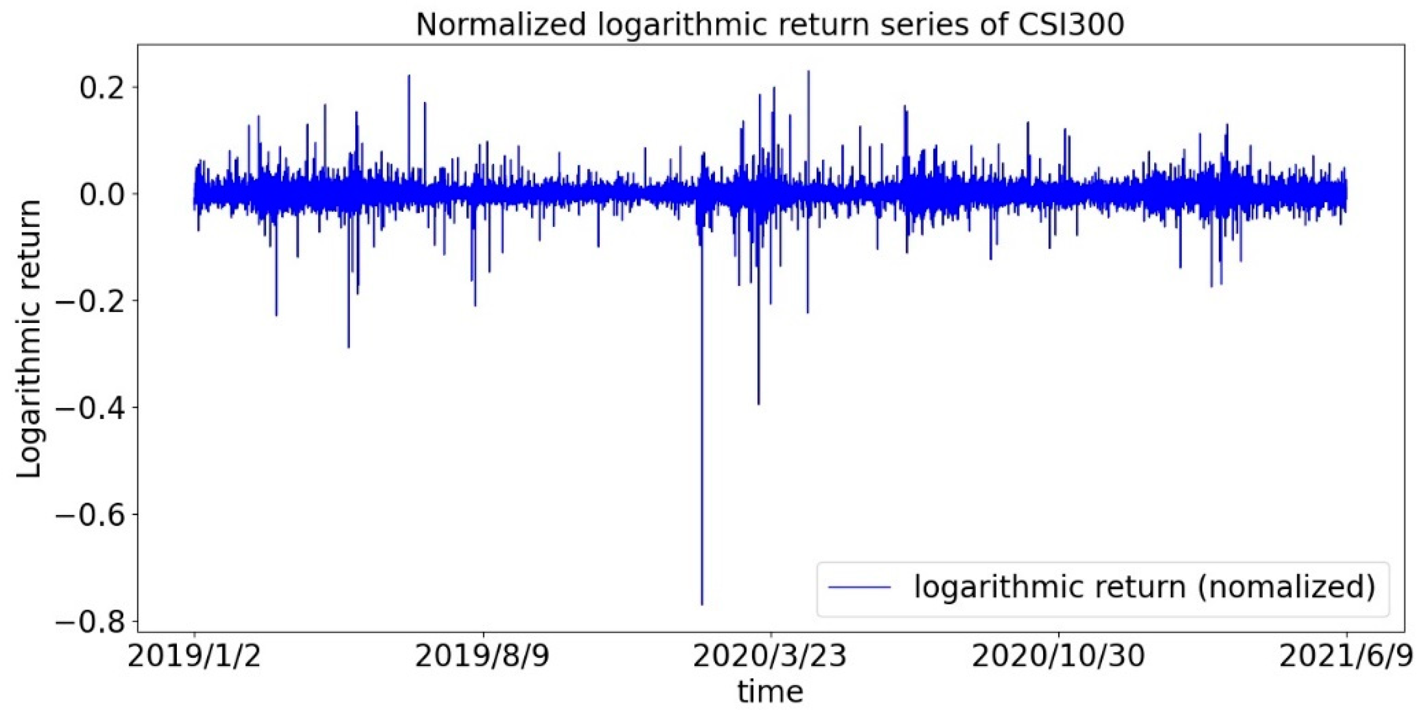
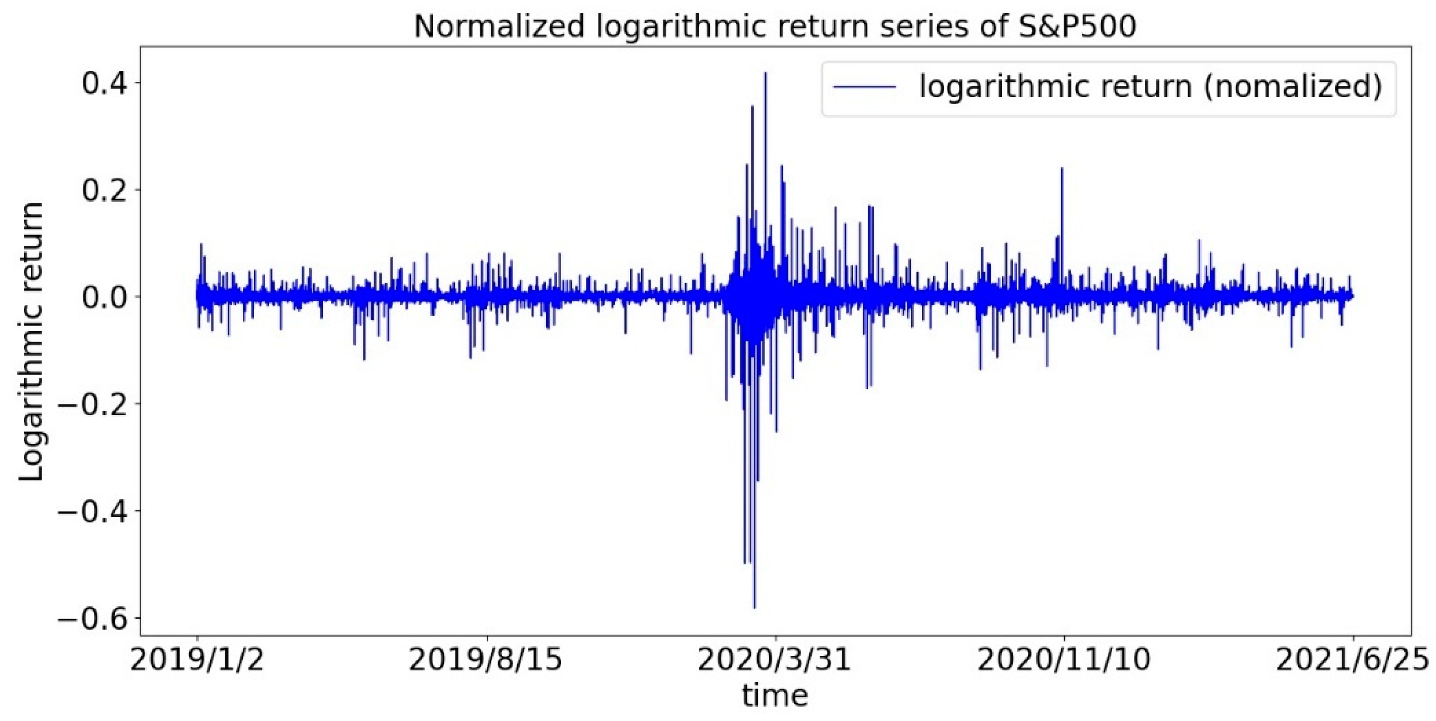
First, we draw the return sequences of the CSI300 Index and the S&P500 Index as shown in
Figure 1 and
Figure 2. It can be roughly seen that the return is not evenly distributed, but there is a phenomenon of volatility clustering, especially during the first panic period of the pandemic. Therefore, we assume that the sequence of returns does not obey a normal distribution.
Then, we calculate the statistical indicators of the return series. In addition to common indicators, such as mean value, extreme value, kurtosis and skewness, we also need to compare the degree of volatility clustering in each stage. As early as 1963, the French mathematician Mandelbrot proposed that the variance of financial asset prices has time-varying characteristics, and the variation range is clustered [
39]. Then Engle first proposed Autoregressive Conditional Heteroskedasticity (ARCH) model to analyze the characteristics of price fluctuation [
40]. Many scholars have confirmed the reliability of the model through empirical analysis [
41,
42,
43]. In this paper, GARCH (1,1) model is used to measure volatility clustering. The model is as follows, and the sum of variable coefficients (
in the variance equation is between 0 and 1. The closer it is to 1, the greater the degree of clustering:
Table 1 shows the descriptive statistics of the two stock index markets in the three stages: before, during and after the first panic period of pandemic. The following conclusions are obtained through analysis:
For the Chinese stock market, represented by the CSI300 Index, at each stage of the pandemic, the kurtosis of the return distribution is significantly greater than the standard value of the standard normal, indicating that the phenomenon of spikes and thick tails in the sequence always exists. Judging from the P-value of the Jarque-Bera test, the hypothesis of the standard normal distribution is strongly rejected, so, we concluded that the stock index market does not conform to the assumption of the traditional financial market, and it is necessary to study market efficiency from a fractal perspective. In addition, the pandemic has indeed had an impact on the market: (1) The coefficient of variation increased significantly during the pandemic, indicating the intensification of dispersion; (2) The skewness becomes smaller, indicating the degree of leftward deviation of the return distribution has increased; (3) kurtosis increases sharply, which indicates that the probability of extreme situations has increased, and the degree of thick tails has deepened; (4) The sum of GARCH (1,1) coefficients becomes larger, indicating that the volatility clustering effect becomes stronger. Above all, it is reasonable to assume that some features of the market have changed.
For the US stock market, which is represented by the S&P500 Index, the spike and thick tail phenomenon and the impact of the pandemic are basically the same as the Chinese stock market, but with different degrees. There are two differences during the pandemic period: (1) The coefficient of variation of S&P 500 index increased faster and was much greater than that of CSI300 index; (2) The average return of the S&P500 index was positive, while that of the CSI300 index fell to negative.
In summary, descriptive statistics show us the market conditions at each stage of the pandemic. The most important conclusion is that there are spikes and thick tails and volatility clustering in the return series of the Chinese and American stock markets, which lays the foundation for the following fractal analysis.
2.3. Method of Testing Fractal: OSW-MF-DFA
The classic method of studying multifractal features is the multifractal detrended fluctuation analysis (MF-DFA) proposed by Kantelhardt in 2002 [
13]. This method is extended by DFA and can be used to analyze the multifractal features of non-stationary time series. Its principle is to eliminate the local trend by dividing the sub-intervals, then fit the wave function of the residual series, and finally explore the power-law correlation of the wave function. We can obtain the generalized Hurst exponent to characterize the multifractal characteristics. However, the non-overlapping of the divided intervals may cause false fluctuations. Therefore, this paper adopts the overlapping smoothing window optimization method which has been verified by many scholars [
23,
24] and is called OSW-MF-DFA method. The specific steps are as follows:
- (1)
Suppose
R (
i) (
i = 1, 2, …,
N) is a certain time series, and
N is the length of the series. First calculate the mean of the series, and construct the cumulative deviation series
Y(
j) as follows:
- (2)
Divide Y(j) into subintervals with a unit length of s. The length of the overlapping part of adjacent intervals is l, which is the only improvement to the original method. Combined with previous experience, the value of l is usually .
- (3)
For each subinterval, fit the univariate linear equation by the least square method. Then eliminate the local trend of each subinterval
v (
v = 1,2, …
Ns), and get the detrending residual sequence
is the local polynomial fitted value and we choose linear univariate polynomials:
- (4)
Calculate the square mean and
-order volatility function of the residual sequence of
Ns subintervals, respectively:
- (5)
Determine the scale index of the volatility function, and get the relationship between
Fq (
s) and
s. If
Fq (
s) is a power-law distribution, the following formula is satisfied when
is constant:
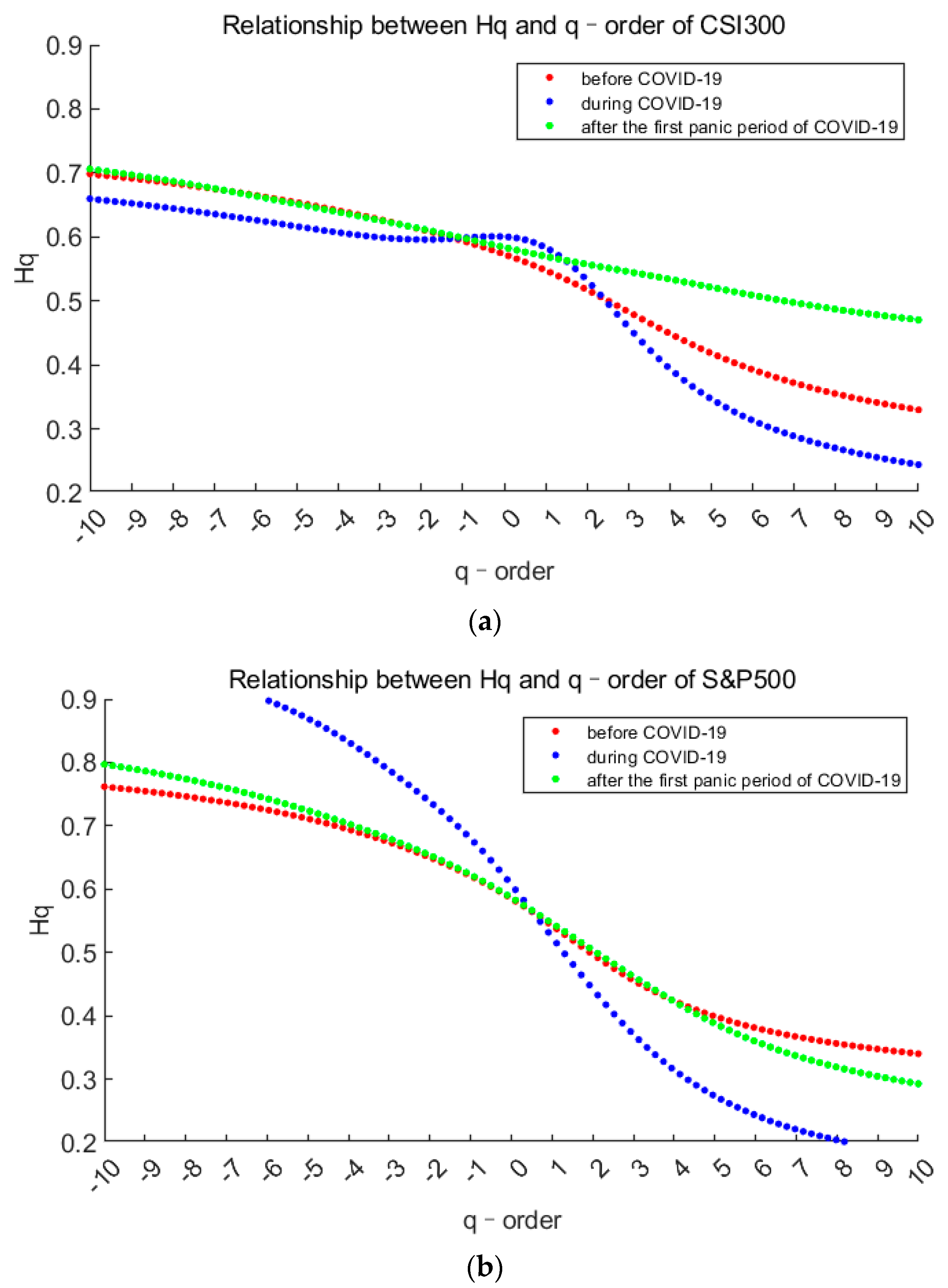
The above formula is linearly fitted in the double logarithmic coordinate system, and the slope h(q) can be obtained, which is called the generalized Hurst exponent. It is used to describe the regional fractal changes of multifractals. Change the order q, repeat the above operation, observe the change of h(q):
- (a)
h(q) does not change with the increase or decrease of q, it is a single fractal system, otherwise it is multifractal.
- (b)
When q < 1, h(q) describes the fractal characteristics of small fluctuations; when q > 1, h(q) describes the fractal characteristics of large fluctuations; when q = 2, h(2) is the classical Hurst index, which measures long memory of the sequence as a whole.
- (c)
h(q) > 0.5 indicates that the sequence is persistent, 0 < h(q) < 0.5 indicates anti-persistence, h(q) = 0.5 indicates that the sequence is a random walk.
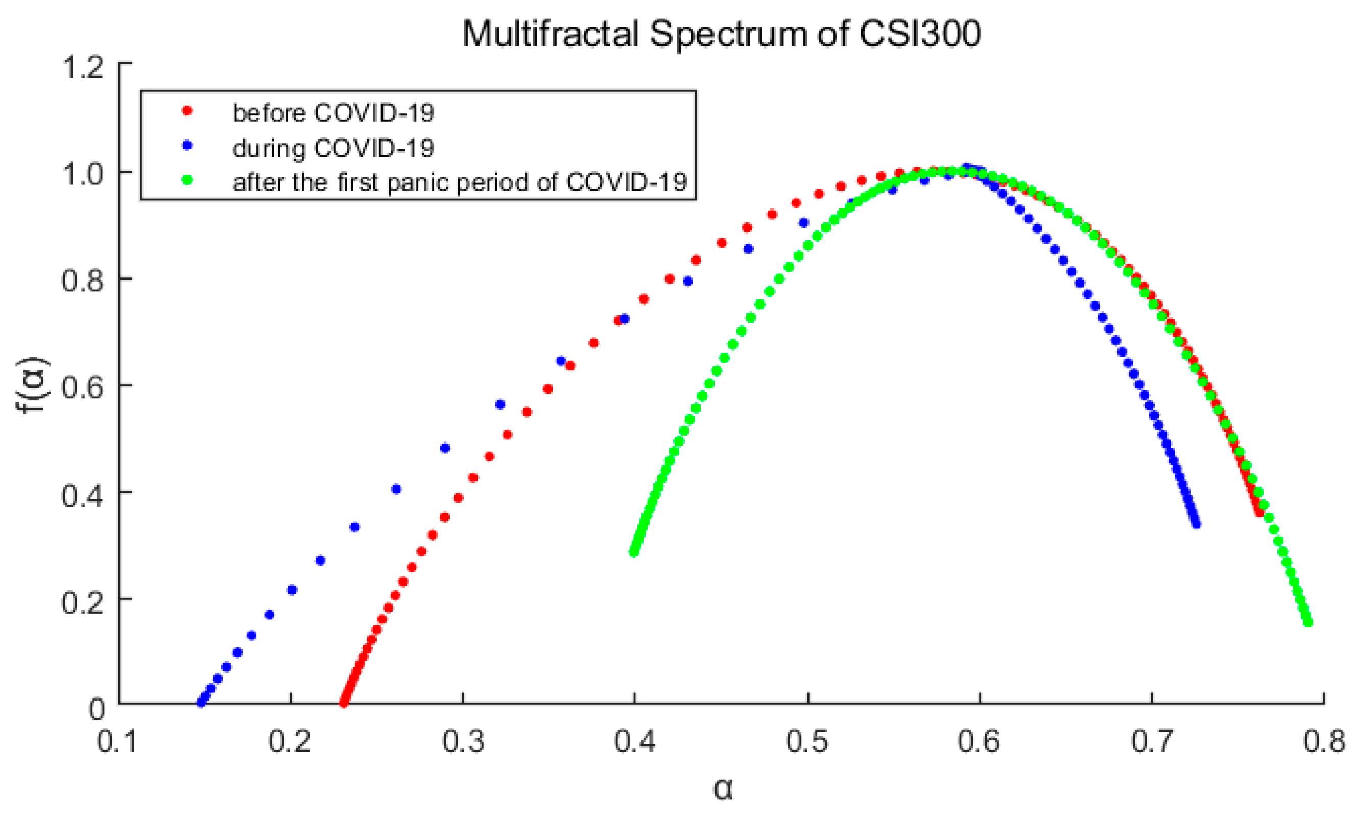
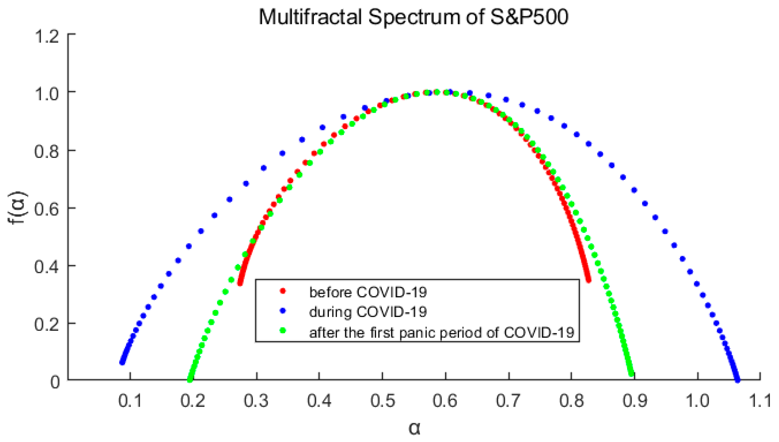
In addition to judging the multifractal by the change of the generalized Hurst index, the multifractal spectrum can also be drawn to further study the sensitivity of the time series to the large and small fluctuations. The multifractal spectrum characterizes the relationship between
f(
α) and α, and its calculation formula is as follows:
Among them, α is the local Hölder index, which is used to describe the degree of variation of the time series, so it is also called the singular index. is called the Renyi index, which is another manifestation of the generalized Hurst index. f(α) is multifractal spectrum. The multifractal spectrum essentially reflects the same fractal characteristics as the generalized Hurst exponent, and has correspondence. The spectrum shape indicates the degree of fluctuation of the sequence. The wider the spectrum shape (that is the greater , the more intense the sequence fluctuation, the more uneven the internal distribution, and the greater the slope of the corresponding Hurst exponent with the order.
2.4. Price Prediction Model: GRU Neural Network
Summarizing the research conclusions of other scholars, it is found that nonlinear neural networks have outstanding performance in prediction. In terms of predicting financial time series, the most popular ones are Long Short-term Memory Neural Network (LSTM) and Gated Recurrent Unit (GRU) [
29,
30,
31,
32,
33,
34,
35]. The latter was proposed by Cho et al., in 2014 and it is a variant of LSTM [
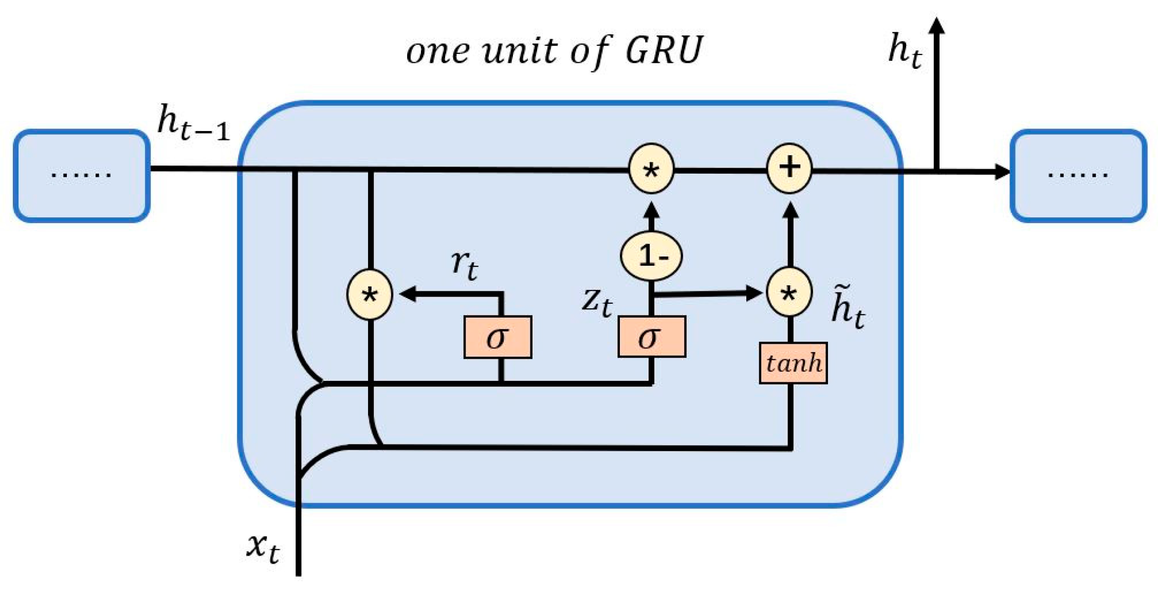
34]. The main change is that the “cell state” that transmits information is removed, but it can also achieve the effect of transmitting long-term memory. This paper selects GRU as the prediction model, and its unit structure diagram is shown in
Figure 3.
In
Figure 3,
xt is the input value at the current moment.
is the output at the previous moment.
is the hidden state at the current moment.
ht is the output at the current moment.
rt and
zt are the reset gate and the update gate respectively, and the former determines how much of the hidden state
at the previous moment needs to be forgotten, the latter controls the extent to which the information of the previous state is passed into the current state.
is the activation function to ensure that the output result is between −1 and 1.
W and
U are the weights of information transmitted between each node. The relationships between the variables are as follows:
4. Conclusions and Discussion
In this paper we take CSI300 and S&P500 as examples to study the fractal properties of 5 min stock indices under the impact of the pandemic and add the fractal features to the GRU neural network for price prediction. The research period is from 1 January 2019 to 9 June 2021. According to the development of the pandemic, it is further divided into three stages before, during and after the first panic period of pandemic. Our study has the following important conclusions: In terms of fractal research, we use OSW-MF-DFA to test the multifractal properties of the market return time series. We find that: (1) Multifractals are always present in all three stages of the two markets, but there are differences in the fractal characteristics of different markets and different stages. Our results show that the multifractals of the two markets have increased significantly during the pandemic, and the US market has been more affected by the pandemic. (2) After the first panic period of pandemic, the fractal degrees of two markets have declined, but they are still higher than the ones before the pandemic. In terms of price prediction, we set three sets of inputs to study the prediction effect of Hurst index and compared to volatility. The research found that: (1) For CSI300 and S&P500, can significantly reduce the forecast error during the large volatility clustering period (during the pandemic), especially for the S&P500 market. (2) The forecast error of S&P500 is significantly greater than that of CSI300, indicating that there are differences in the characteristics of the Chinese and American stock markets.
This study also has some suggestions for market agents. For market participants, it provides a way to judge the current market efficiency through fractal analysis. This study shows that Hurst index may be a good timing index and adding fractals can make predictions more accurate during the panic period of market. For policy makers, it has become a new method to study the intervention degree of fiscal and monetary policy on the market through fractal situation. For regulators, such as exchanges and CSRC, they can supervise the operation of the current market from the perspective of multifractal. When the efficiency of the market is reduced due to a major impact such as the pandemic, the trading rules could be modified appropriately to improve the stability of the market.
Our work is a study on the fractal and forecast of the market under the impact of the pandemic. By adding Hurst index as an input element in the GRU neural network, we improved the forecast accuracy during the panic period. But before and after that it is not contribute to the prediction accuracy, so the future research can join a dynamic system to determine whether to add the Hurst index when forecasting.


